Statistical permutation quantifiers in the classical transition of conservative-dissipative systems
Abstract
We study the behavior of a nonlinear semiclassical system using Shannon entropy and two approaches to statistical complexity. These systems involve the interaction between classical variables (representing the environment) and quantum ones. Both conservative and dissipative regimes are explored. To calculate the information metrics, probability distributions are derived from the temporal evolution via the Bandt-Pompe permutation method. Additionally, we describe the classical limit in terms of a motion invariant linked to the uncertainty principle. Our analysis reveals three distinct regions, including a mesoscopic one, along with other notable findings.
Keywords: Nonlinear semiclassical systems, Shannon entropy, Statistical complexity, Bandt-Pompe method, Classical-quantum interaction, Mesoscopic regimes.
1 Introduction
The emergence of the classical world from the quantum domain is a topic of significant interest, both theoretically [1, 2, 3] and experimentally [4, 5, 6], as well as for its practical applications. The decoherence process [7], for instance, is closely linked to mesoscopic physics a field focusing on materials of intermediate scales. Mesoscopic systems, such as those used in nanotechnology, serve as practical examples [8, 9, 10, 11]. Additionally, semiclassical systems have been extensively employed over the years to address various physical problems [12, 13, 14, 15, 16, 17, 18, 19, 20, 21, 22, 23].
We have investigated systems that exhibit the coexistence of quantum and classical variables [24, 25, 26, 27, 28, 29, 30]. In these systems, the classical variables serve as a representation of the reservoir interacting with the quantum system.
Within this framework, we have explored the classical limit of quantum systems by employing a motion invariant associated with the Heisenberg Principle. Our approach includes dynamic analyses [24, 25, 26, 27, 28, 30] and the application of various tools from Information Theory (IT) [31, 32].
The classical limit of the system addressed in this work was previously examined in Ref. [30], utilizing Poincaré sections and analyzing the temporal evolution of key quantities. Both conservative and, for the first time, dissipative regimes were considered. In this study, we revisit the problem by employing Shannon entropy and two definitions of statistical complexity: the LMC complexity [33] and the Jensen-Shannon complexity [34]. To compute any information quantifier, a probability distribution function is required. For this purpose, we apply the Bandt-Pompe permutation based symbolic method [35], recognized for its efficiency in capturing key features of various time series [36, 37, 38, 39, 40, 41].
Our objective is to gain a deeper understanding and characterization of the process, uncovering details that cannot be obtained using dynamic tools alone.
2 The semi-classical model and classical limit
We consider a Hamiltonian of the form
| (1) |
In this Hamiltonian, and are considered quantum operators while and canonically conjugated classic variables. is the Identity operator. and are frequencies and a positive parameter positive [24]. The non-linear quantum-classical interaction appears through the term in (1). The semiclassical methodology that we use, is developed in the Appendix. The equations of motion that govern the system, as demonstrated in Ref. [30], are given by the following set of coupled non-linear equations
| (2) | ||||
To study the classical limit of the system (LABEL:eq_semi), we need to compare with the solutions corresponding to the classical analogous of the Hamiltonian (1) [26]
| (3) |
By Hamilton’s equations we obtain (see Appendix)
| (4) | ||||
We define as
| (5) |
is a motion-invariant for the systems (LABEL:eq_semi) in both regimens (conservative and dissipative) (see [24, 30]) and is related to the uncertainty principle describing the deviation with respect to classicity, a condition characterized by (trivial motion-invariant).
Eqs. (LABEL:eq_semi) do not explicitly depend upon while mean values depend on it via the initial conditions through satisfying (5). The inequality (5) and its classical value, are crucial in our study of the classical limit , as will be seen throughout the article.
Focus now attention upon the relative energy .
| (6) |
where is the total energy. is also a motion invariant that verifies due to the uncertainty principle. corresponds to the minimum value and represents the totally quantum case. is dimensionless. The LC is , i.e.,
| (7) |
In the dissipative case we replace, in (6), by [30]. Our main interest lies in the evolution of observable when grows from its minimum unity value .
3 Bandt-Pompe method
To calculate our Information quantifiers, it is necessary to have a probability distribution associated with the data series that one wants to analyze. In this case, of a time series of the semiclassical and classical systems. We obtain this probability distribution function (PDF) using the Bandt and Pompe method [35]. This methodology basically consists of a symbolization process that is described as follows: Let be an arbitrary time series, the first step is to divide the time series into overlapping partitions comprising observations separated by time units. For given values of and , each data partition can be represented by
| (8) |
where is the partition index. The parameters and are the so-called embedding dimension and the embedding delay, respectively, the only two parameters of the Bandt and Pompe method. The original proposal presented by Bandt and Pompe was limited to , this means that the data partitions comprised consecutive elements of time series, however, Cao et al. [42], Zunino et al. [43] and Pessa and Ribeiro [44], studied the embedding delay for values greater than 1.
Then, for each partition we evaluate the permutation of the index numbers which arranges the elements of in ascending order, that is, the permutation of the index numbers defined by the inequality . In case of equality of values, the order of appearance of the elements of the partition is maintained, i.e., if , then for . After evaluating the permutation symbols associated with all data partitions, a symbolic sequence is obtained.
The ordinal probability distribution is the relative frequency of all possible permutations within the symbolic sequence
| (9) |
Here represents each of the different ordinal patterns.
The Bandt Pompe method has desirable features (i) simplicity, (ii) extremely fast calculation-process, and (iii) robustness. It is also invariant with respect to non-linear monotonous transformations. This method can be applied to any type of time series (regular, chaotic, noisy, or experimental) [31].
4 Information Quantifiers
4.1 Shannon permutation entropy
The Shannon permutation entropy is defined as follows
| (10) |
where the probability distribution is obtained using the Bandt and Pompe method. Permutation entropy quantifies the randomness in the ordering dynamics of a time series. This means that implies completely regular behavior, while indicates behavior with maximum disorder [35, 44].
The normalized permutation entropy adopts the form
| (11) |
where y .
4.2 LMC-statistical complexity
In 1995, Lopez-Ruiz, Mancini and Calbet (LMC) [33, 45], proposed a measure of complexity given by the following expression
| (12) |
where is known as the disequilibrium factor and is defined as a distance (Euclidean or 2-norm distance) between a probability distribution and the equiprobable distribution , with . Disequilibrium gives us a way to measure how “separate” the probability distribution of the system under treatment is from the uniform distribution, which gives us maximum uncertainty of the state of the system.
4.3 Jensen Shannon-statistical complexity
The Jensen Shannon-statistical complexity (JSC) [34] is based on the pioneering Statistical complexity of López-Ruiz et al. The fundamental difference between these two quantities lies in how distances are measured in the probability space. The JSC is defined as the product of the permutation entropy and the Jensen-Shannon divergence between the ordinal distribution and the uniform distribution instead of Euclidean distance. We also consider the normalized version of the JSC.
| (13) |
where
| (14) |
is the Jensen-Shannon divergence [46] and
| (15) |
is a normalization constant.
5 Results
To solve the equations (LABEL:eq_semi) and (4) we choose the following parameter values: . While for the initial conditions we take .
For the conservative system (), we choose . In the dissipative regimen we take the same value for the initial energy value . In both regimes we fixed this values, as we set () in (6). In the dissipative cases is .
We select , where . For the classic case is , which results from taking the value in the previous expression. By appeal to (5) we see that ( in the classical instance). In addition, from (1) we deduce via
evaluating all quantities at the initial time. We have also an equivalent expression for the classical analogous system.
In the numerical calculation of the Shannon permutation entropy and the statistical complexities, the Python package ordpy developed by Arthur A. B. Pessa and Haroldo V. Ribeiro [44] was used. We have employed the values and for the dimensional embedding and embedding delay, respectively. The results have been conceptually confirmed using .
The time series for the semiclassical case, have been constructed with the values of , each one for a different value of (or ). Also we have considered in the classical scenario (), the unique series formed by the values. In both cases to we have taken points for each series. The condition is verified [31].
In all figures we observe low values of the information quantifiers, unlike what we have found for the chaotic Hamiltonian of Refs. [31, 32]. This feature are consistent with the regularity observed in the Poincaré Sections [30]. In detail, after the jump observed in the quasi-quantum zone between and (see below), one finds a very small band of variation of the values. However, the three regions of Refs. [31, 32] of the path to the classical analogous, continues being observed (quasi-quantum, transitional and classical).
It is convenient an analysis with additional tools such as information quantifiers, which, as mentioned, have proven efficiency for this type of problem.
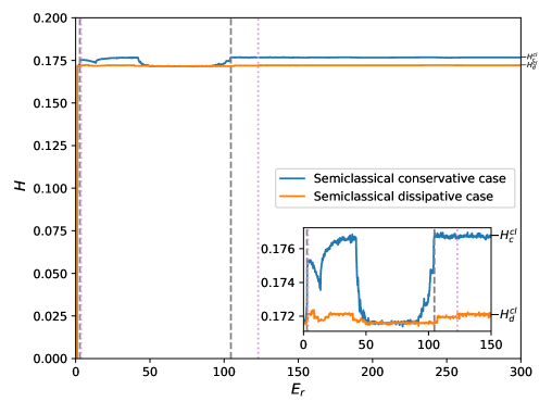
In Fig.1 we plot the normalized Entropy vs. the relative energy , for both conservative and dissipative regimes. In the conservative case (blue curve), between and , we find out a zone, what we can call quasi-quantum. In the zone , with dynamic tools, quasi-periodic behavior has been observed (remember that is the lowest possible value of and corresponds to the fully quantum case). At (first gray colored vertical dashed line), we have observed on a logarithmic scale, a drastic change (taking into account the mentioned small band of variation of ). The transition zone (mesoscopic) can be set between the values and and finally the convergence zone to the classical analogous value , can be seen from (second gray discontinuous vertical line).
The equivalent zones corresponding to the dissipative regime (orange curve) are: quasi-quantum from to (first plum colored vertical dashed line), the transitional from to , and the convergence zone to the analogous classic case from (second plum colored vertical dashed line). , is the value of the entropy of the classical analogous in the dissipative case (remember that in this regime we replace in (6), by ).
Additionally, the figure contains an inset in which the morphology of the curves in the transition zone is observed in detail. This region can be associated with a mesoscopic one, due to the important presence of quantum features. The zone of convergence to the totally classical system must correspond to a decoherence process [29].
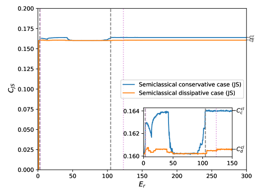
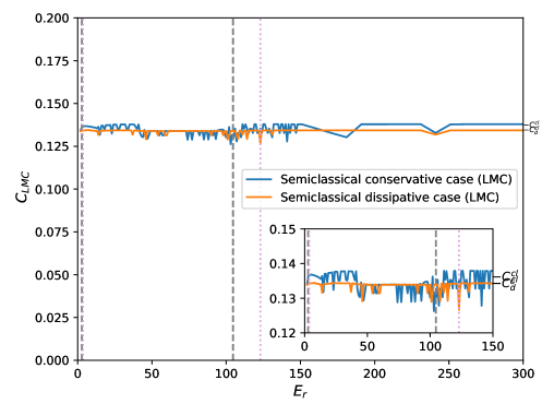
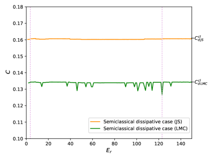
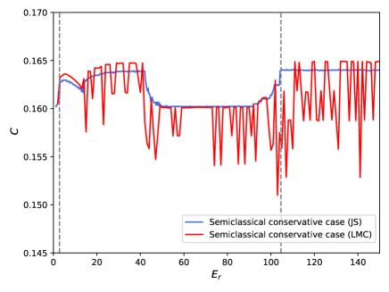
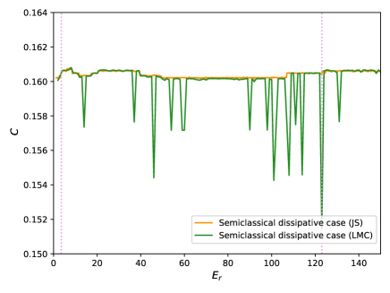
In Figs. 2 we plot the two definitions of the statistical complexity vs. . In both figures, one can clearly notice the three zones mentioned in Fig.1. These results are the same for both and . The blue curve corresponds to the conservative case and the orange curve to the dissipative one. The dashed vertical lines indicate the transition zone, gray for the conservative regime (between ) and plum for the dissipative case (from to ). Furthermore, in each graph there is a inset that basically consists of an increase in scale of the original graph, showing the transition zone. In Figure 2(a) we can see the statistical complexity of Jensen-Shannon . and are the statistical complexity values of the classical analogous of the conservative and dissipative regimes, respectively. Figure 2(b) presents the statistical complexity introduced by Lopez-Ruiz et al. vs . The blue and the orange curves are associated to the conservative and dissipative system, respectively. In this case, and are the values of the statistical complexity of the classical analogous (conservative and dissipative regimen).
5.1 Comparing outcomes.
As we have already commented, all figures show convergence towards the values of the corresponding classical analogous. Except for fluctuations, in general the results corresponding to the conservative regime are slightly higher than those of the dissipative regime. A result that can be expected since the dynamics of the system is regular in both regimes. However, contrary to what one might think a priori, convergence start earlier in the conservative case. The zones are the same for the entropy and the complexities and . Transitional zone of the conservative regime is (), while for the dissipative case it is ().
Note that the representative figures of and are similar but with a difference in scale. This is because the disequilibrium remains almost constant around its mean value (conservative) and (dissipative), for all values of . In the case of the complexities , the disequilibrium is also quasi-constant as a function of , but it has greater fluctuations around its mean value and (conservative and dissipative dynamics).
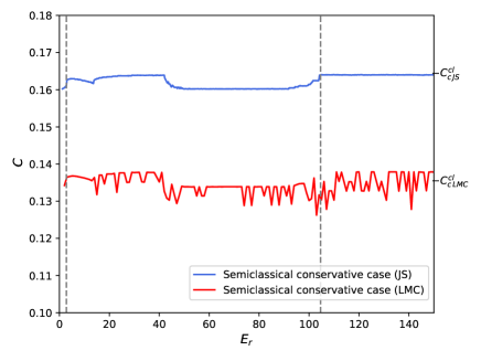
Figures 3(a) and 3(b) are comparative graphs between and for both regimes. The behavior of the curve of is more erratic that the one (due to and behaviours). This happens for both the conservative and dissipative systems. On the other hand, the different criteria used to normalize the disequilibrium in the expressions of and cause a difference in scale. Figures 4(a) and 4(b), expose this characteristic for the conservative and dissipative regimes, respectively. To achieve a meaningful comparison, it was convenient to apply a translation to the complexity by multiplying all values of the curve by the factor . It is observed that, despite the marked fluctuations in the amplitude of compared to , both exhibit a similar profile. This phenomenon highlights the consistency in the underlying behavioral pattern.
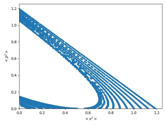
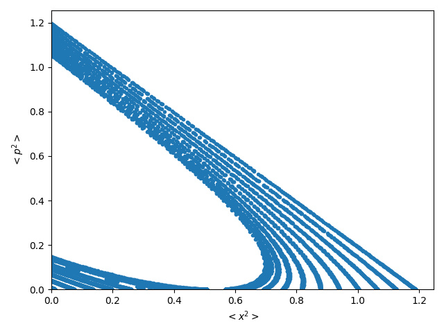
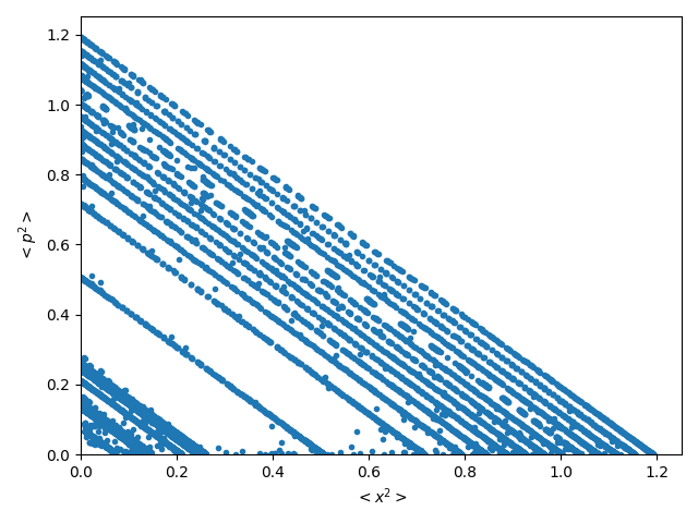
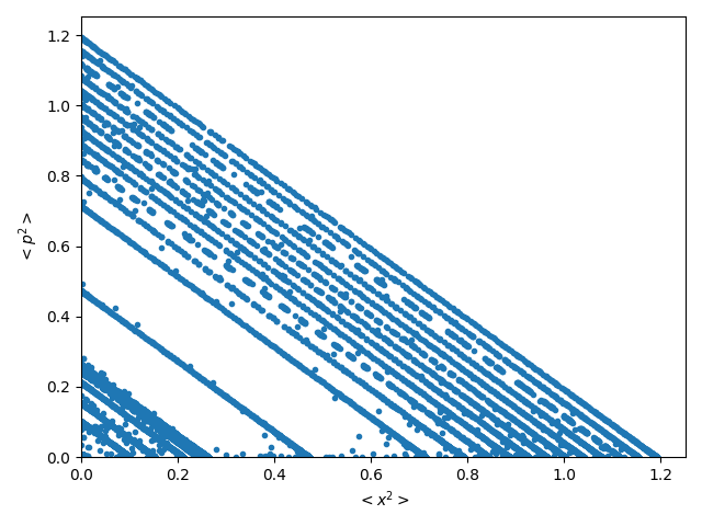
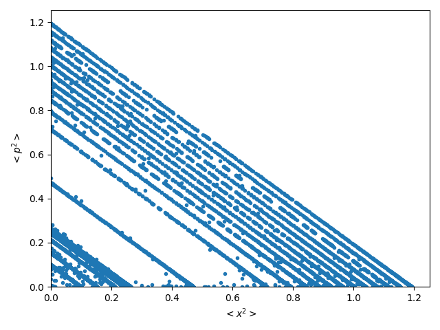
In Figures 5 and 6 we represent the Poincaré sections (conservative regime) and the projections of the Poincaré sections (dissipative dynamics) (for more details see [30]), suitable for the results obtained in this work.
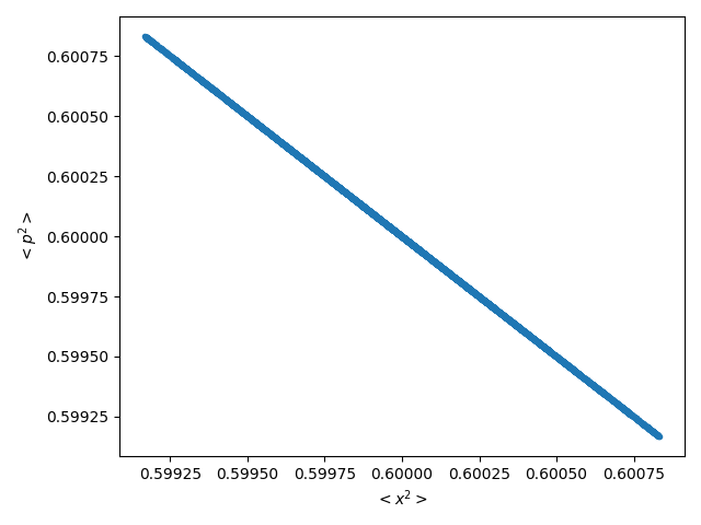
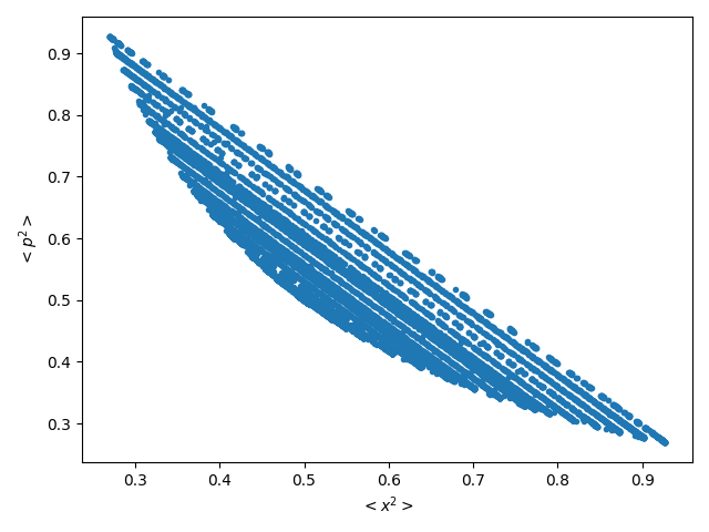
In Figure 5 we plot Poincaré sections corresponding to (a) and (b) , both in the semiquantum zone, (c) belonging to the transition zone, (d) , the critical point between the transition and classical zones where convergence begins, (e) in the classical zone. Finally in (f) we depict the Poincaré section of the conservative classical analogous.
Figure 6 shows the projections of the 3D dissipative Poincaré sections, for the same values in the same zones as figure 5 ([30]), in subfigures (a), (b), (c) and (e). Subfigure (d) correspond to the critical point for the disipative regime . In (f) we plot the projection of the 3D Poincaré section of the dissipative classical analogous.
It is important to observe in these figures the difficulty in precisely defining, using Poincaré Sections, the limit between the three zones. This happens because of the system dynamics is very regular. However, the information quantifiers used in this work offer better differentiation.


6 Conclusions
In this article we have analyzed the conservative and dissipative dynamics of the semiclassical Hamiltonian (1), which contains both quantum and classical variables. For this we have used information quantifiers, such as the Shannon entropy and the Statistical complexity. In the case of the latter, we analyze two versions, the pioneer one introduced by Lopez-Ruiz et al. [33, 45] and the Jensen Shannon complexity [34]. The probability distribution to evaluate all these quantities was extracted from the time series using the Bandt and Pompe permutational method [35]. A methodology that has proven to be robust and reliable. In particular we have studied the classical limit of the system, that is, the convergence to the classical analogue of represented by Eq. (3) (only with classical variables), as a function of the relative energy (6), related to the Uncertainty Principle, with .
In [30] we had studied the same problem, but using dynamic tools such as Poincaré sections and projections of 3D Poincaré sections. The result found was the existence of three zones, quasi-quantum, transitional and finally one where the convergence to the results corresponding to the classical analogue was observed (classical zone). However, the boundaries between zones were diffuse, because the dynamics of the system is regular (see figures 5 and 6). The regularity of the dynamics is reflected in the figures of the present article, by their low values of all information quantifiers. Moreover, after the jump observed in the quasi-quantum zone, one finds a very small band of variation of the respective values.
It is seen in Figs. 1, 2, 3 and 4 that the Shannon permutation entropy and the statistical complexities and confirm the mentioned three zones of the process (quasi-quantum, transitional or mesoscopic and that of decoherence, convergent to the classical analogous result). The corresponding intervals of are the same for the three quantifiers and can be synsetized by the transitional zone. In the conservative scenario and in the dissipative regime .
We have found that the figures of and have similar morphology but with a difference in scale. This is because the disequilibrium remains almost constant for all values of in both scenarios, conservative and dissipative. Disequilibrium corresponding to the complexity is also quasi-constant, but it has greater fluctuations around its mean value (conservative and dissipative regimes).
We conclude that the information quantifiers used in this work provide more details about the convergence process of the semiclassical system to the classical analogous, confirming the results obtained with the Poincaré sections used in Ref. [30], but with greater precision.
Appendix A Appendix
A.1 Semiclassical Model
Our semiclassical Hamiltonian is (1). In our methodology, the time evolution of all operator is the canonical one. The Hamiltonian also depends upon the classical variables and , which represent the reservoir. These classical quantities obey Hamilton’s equations, of course, where the temporal generator is the mean value of the Hamiltonian [26, 49]. If we add to the system an appropriate ad hoc term we get dissipation [24, 25, 28].
Thus, for a given operator we have
| (A1) |
The evolution of is provided by
| (A2) |
using a suitable density operator .
can always be cast as [50, 51]
| (A3) |
where we can have . We are interested in finite -values. In this case it is said that the set of operators , close a Lie semialgebra with [50, 51]. For a semiclassical Hamiltonian like (1), the coefficients depend on and . For classical variables one
| (A4a) | |||
| (A4b) | |||
where if our system is dissipative. Instead, if , it is conservative.
To verify these features [24, 25, 28] a particularly convenient space is used. We will call it “-space”. With respect to it, a bunch of equations deduced from Eqs. (A2) and (A4) conform an autonomous set of equations. They are first-order coupled differential ones, of the type [24, 25, 28]
| (A5) |
with is a “vector”. It is regarded as a variable containing both classical and quantum parts. We consider volume elements of this space, surrounded by a surface . The dissipative term generates a contraction of [52]. The divergence of our vector is seen to be , given the fact that the matrix in equations (A3) is traceless. This happens due to the canonical character of Eqs. (A1). Consequently. we must have [24, 25, 28]
| (A6) |
Accordingly, we deal with a dissipative system [52]. If the classical Hamiltonian is of the form
| (A7) |
then the time-evolution of the total energy becomes
| (A8) |
Its meaning is to be ascertained through the lens of Eq. (A6) [24, 25, 28].
The complete set of equations (A2) + (A4) constitutes an autonomous set of non-linear coupled first-order ordinary differential equations (ODE). They allow for a dynamical description in which no quantum rules of the sub-quantal system are violated, e.g-, the commutation-relations are trivially conserved at all times, since the quantum evolution is the canonical one for an effective time-dependent Hamiltonian ( and , play the role of time-dependent parameters of the quantum system).
The initial conditions are determined by a suitable quantum density operator . This happens both in the dissipative and in the conservative instances [27, 28].
References
- [1] Struyve, W. (2020). Semi-classical approximations based on Bohmian mechanics. International Journal of Modern Physics A, 35(14), 2050070.
- [2] Brack, M., & Bhaduri, R. (2018). Semiclassical physics. CRC Press.
- [3] Arndt, M., Hornberger, K., & Zeilinger, A. (2005). Probing the limits of the quantum world. Physics world, 18(3), 35.
- [4] Li, X. Q., Luo, J., Yang, Y. G., Cui, P., & Yan, Y. (2005). Quantum master-equation approach to quantum transport through mesoscopic systems. Physical Review B, 71(20), 205304.
- [5] Goan, H. S., & Milburn, G. J. (2001). Dynamics of a mesoscopic charge quantum bit under continuous quantum measurement. Physical Review B, 64(23), 235307.
- [6] Barker, J., & Bauer, G. E. (2019). Semiquantum thermodynamics of complex ferrimagnets. Physical Review B, 100(14), 140401.
- [7] Joos, E., Zeh, H. D., Kiefer, C., Giulini, D. J., Kupsch, J., & Stamatescu, I. O. (2013). Decoherence and the appearance of a classical world in quantum theory. Springer Science & Business Media.
- [8] Das, M. P. (2010). Mesoscopic systems in the quantum realm: fundamental science and applications. Advances in Natural Sciences: Nanoscience and Nanotechnology, 1(4), 043001.
- [9] Brandes, T. (2005). Coherent and collective quantum optical effects in mesoscopic systems. physics reports, 408(5-6), 315-474.
- [10] Iachello, F., & Zamfir, N. V. (2004). Quantum phase transitions in mesoscopic systems. Physical review letters, 92(21), 212501.
- [11] Guo, L. Z., Zheng, Z. G., & Li, X. Q. (2010). Quantum dynamics of mesoscopic driven Duffing oscillators. Europhysics Letters, 90(1), 10011.
- [12] Bloch, F. (1946). Nuclear induction. Physical review, 70(7-8), 460.
- [13] Milonni, P. W., Shih, M. L., & Ackerhalt, J. R. (1987). Chaos in laser-matter interactions (Vol. 6). World Scientific Publishing Company.
- [14] Nielsen, S., Kapral, R., & Ciccotti, G. (2001). Statistical mechanics of quantum-classical systems. The Journal of Chemical Physics, 115(13), 5805-5815.
- [15] Micklitz, T., & Altland, A. (2013). Semiclassical theory of chaotic quantum resonances. Physical Review E, 87(3), 032918.
- [16] Cosme, J. G., & Fialko, O. (2014). Thermalization in closed quantum systems: Semiclassical approach. Physical Review A, 90(5), 053602.
- [17] Prants, S. V. (2017). Quantum–classical correspondence in chaotic dynamics of laser-driven atoms. Physica Scripta, 92(4), 044002.
- [18] Ribeiro, R. F., & Burke, K. (2018). Deriving uniform semiclassical approximations for one-dimensional fermionic systems. The Journal of Chemical Physics, 148(19).
- [19] Graefe, E. M., Höning, M., & Korsch, H. J. (2010). Classical limit of non-Hermitian quantum dynamics—a generalized canonical structure. Journal of Physics A: Mathematical and Theoretical, 43(7), 075306.
- [20] Bastarrachea-Magnani, M. A., Lerma-Hernández, S., & Hirsch, J. G. (2014). Comparative quantum and semiclassical analysis of atom-field systems. II. Chaos and regularity. Physical Review A, 89(3), 032102.
- [21] Allori, V., & Zanghì, N. (2009). On the classical limit of quantum mechanics. Foundations of Physics, 39, 20-32.
- [22] Kurchan, J. (2018). Quantum bound to chaos and the semiclassical limit. Journal of statistical physics, 171(6), 965-979.
- [23] Oliveira, A. C., Nemes, M. C., & Romero, K. F. (2003). Quantum time scales and the classical limit: Analytic results for some simple systems. Physical Review E, 68(3), 036214.
- [24] Kowalski, A. M., Plastino, A., & Proto, A. N. (1995). Semiclassical model for quantum dissipation. Physical Review E, 52(1), 165.
- [25] Kowalski, A. M., Plastino, A., & Proto, A. N. (1997). A semiclassical statistical model for quantum dissipation. Physica A: Statistical Mechanics and Its Applications, 236(3-4), 429-447.
- [26] Kowalski, A. M., Plastino, A., & Proto, A. N. (2002). Classical limits. Physics Letters A, 297(3-4), 162-172.
- [27] Kowalski, A. M., & Rossignoli, R. (2018). Nonlinear dynamics of a semiquantum Hamiltonian in the vicinity of quantum unstable regimes. Chaos, Solitons & Fractals, 109, 140-145.
- [28] Kowalski, A.M.; Plastino, A., Asger S. Thorsen (Ed.). (2020), Semiquantum Time evolution. Classical limit. Nova.
- [29] Kowalski, A. M., Plastino, A., & Gonzalez, G. (2021). Classical chaos described by a Density matrix. Physics, 3(3), 739-746.
- [30] Gonzalez Acosta, G., Plastino, A., & Kowalski, A. M. (2023). Dynamical classic limit: Dissipative vs conservative systems. Chaos: An Interdisciplinary Journal of Nonlinear Science, 33(1), 013126.
- [31] Kowalski, A. M., Martín, M. T., Plastino, A., & Rosso, O. A. (2007). Bandt–Pompe approach to the classical-quantum transition. Physica D: Nonlinear Phenomena , 233 (1), 21-31.
- [32] Kowalski, A. M., Martín, M. T., & Plastino, A. (2015). Generalized relative entropies in the classical limit. Physica A: Statistical Mechanics and its Applications, 422, 167-174.
- [33] Lopez-Ruiz, R., Mancini, H. L., & Calbet, X. (1995). A statistical measure of complexity. Physics letters A, 209(5-6), 321-326.
- [34] Lamberti, P. W., Martin, M. T., Plastino, A., & Rosso, O. A. (2004). Intensive entropic non-triviality measure. Physica A: Statistical Mechanics and its Applications, 334(1-2), 119-131.
- [35] Bandt, C., & Pompe, B. (2002). Permutation entropy: a natural complexity measure for time series. Physical review letters, 88(17), 174102.
- [36] Keller, K., & Sinn, M. (2005). Ordinal analysis of time series. Physica A: Statistical Mechanics and its Applications, 356(1), 114-120.
- [37] Rosso, O. A., Zunino, L., Pérez, D. G., Figliola, A., Larrondo, H. A., Garavaglia, M., & Plastino, A. (2007). Extracting features of Gaussian self-similar stochastic processes via the Bandt-Pompe approach. Physical Review E, 76(6), 061114.
- [38] Saco, P. M., Carpi, L. C., Figliola, A., Serrano, E., & Rosso, O. A. (2010). Entropy analysis of the dynamics of El Niño/Southern Oscillation during the Holocene. Physica A: Statistical Mechanics and its Applications, 389(21), 5022-5027.
- [39] Rosso, O. A., Olivares, F., Zunino, L., De Micco, L., Aquino, A. L., Plastino, A., & Larrondo, H. A. (2013). Characterization of chaotic maps using the permutation Bandt-Pompe probability distribution. The European Physical Journal B, 86, 1-13.
- [40] Aquino, A. L., Cavalcante, T. S., Almeida, E. S., Frery, A. C., & Rosso, O. A. (2015). Characterization of vehicle behavior with information theory. The European Physical Journal B, 88, 1-12.
- [41] Henry, M., & Judge, G. (2019). Permutation entropy and information recovery in nonlinear dynamic economic time series. Econometrics, 7(1), 10.
- [42] Cao, Y., Tung, W. W., Gao, J. B., Protopopescu, V. A., & Hively, L. M. (2004). Detecting dynamical changes in time series using the permutation entropy. Physical review E, 70(4), 046217.
- [43] Zunino, L., Soriano, M. C., Fischer, I., Rosso, O. A., & Mirasso, C. R. (2010). Permutation-information-theory approach to unveil delay dynamics from time-series analysis. Physical Review E, 82(4), 046212.
- [44] Pessa, A. A., & Ribeiro, H. V. (2021). ordpy: A Python package for data analysis with permutation entropy and ordinal network methods. Chaos: An Interdisciplinary Journal of Nonlinear Science, 31(6).
- [45] Lopez-Ruiz, R. (2001). Complexity in some physical systems. International Journal of Bifurcation and Chaos, 11(10), 2669-2673.
- [46] Lin, J. (1991). Divergence measures based on the Shannon entropy. IEEE Transactions on Information theory, 37(1), 145-151.
- [47] Zunino, L., Soriano, M. C., & Rosso, O. A. (2012). Distinguishing chaotic and stochastic dynamics from time series by using a multiscale symbolic approach. Physical Review E, 86(4), 046210.
- [48] Rosso, O. A., Larrondo, H. A., Martin, M. T., Plastino, A., & Fuentes, M. A. (2007). Distinguishing noise from chaos. Physical review letters, 99(15), 154102.
- [49] Cooper, F., Dawson, J., Habib, S., & Ryne, R. D. (1998). Chaos in time-dependent variational approximations to quantum dynamics. Physical Review E, 57(2), 1489.
- [50] Alhassid, Y., & Levine, R. D. (1978). Connection between the maximal entropy and the scattering theoretic analyses of collision processes. Physical Review A, 18(1), 89.
- [51] Levine, R. D., Napoli, D. R., Otero, D., Plastino, A., & Proto, A. N. (1986). Maximum entropy approach to nuclear fission processes. Nuclear Physics A, 454(2), 338-358.
- [52] Arnold, V. I. (2013). Mathematical methods of classical mechanics (Vol. 60). Springer Science & Business Media.