Statistical properties of extreme soliton collisions
Abstract
Synchronous collisions between a large number of solitons are considered in the context of a statistical description. It is shown that during the interaction of solitons of the same signs the wave field is effectively smoothed out. When the number of solitons increases and the sequence of their amplitudes decay slower, the focused wave becomes even smoother and the statistical moments get frozen for a long time. This quasi-stationary state is characterized by greatly reduced statistical moments and by the density of solitons close to some critical value. This state may be treated as the small-dispersion limit, what makes it possible to analytically estimate all high-order statistical moments. While the focus of the study is made on the Korteweg–de Vries equation and its modified version, a much broader applicability of the results to equations that support soliton-type solutions is discussed.
In this communication we show how synchronous collisions between a great number of solitons realize the states with the maximum soliton density which corresponds to the minimal allowed spatial size of the soliton ensemble. Within a broad class of evolution equations these particular states of solitons of the same sign are characterized by new approximate conserved quantities in the form of statistical moments. This happens due to the effective smoothing of the wave field stemming from the great ratio of the nonlinearity vs dispersion parameter. These states correspond to the minimum values of statistical moments for interacting unipolar solitons, which are evaluated analytically.
I Introduction
The soliton turbulence is a challenging topic of recent research which is highly interesting from both, the mathematical and the physical points of view. In physics it describes strongly coherent wave states when the assumptions of a wave (weak) turbulence are violated, and thus the quasi-Gaussian probabilistic description completely fails. In mathematics, it represents deterministic chaos-like behaving systems which are formally solvable by means of the Inverse Scattering Transform, but its machinery is often too much complicated to write down explicit solutions or relations.
The kinetic theory for a soliton gas [1, 2] describes the transport of the soliton spectral density. Due to the failure of a linear superposition property, the kinetic theory cannot help to compute wave fields as such. In particular, the occurrence and probability of extreme events cannot be evaluated. It was shown in Refs. 3, 4 within the Korteweg–de Vries-type equations, that interactions of solitons of the same sign lead to some reduction of the wave field amplitude, whereas collisions of solitons of different signs (which can co-exist in the modified Korteweg – de Vries or the Gardner equations of the focusing types) can produce very high waves (so-called rogue waves). Meanwhile, the question of a meaningful description of the amplitude probability distribution in essentially coherent wave ensembles remains unclear.
It was pointed out recently [5, 6], that the standard definition of the variance
| (1) |
for a sign-defined wave field imposes a formal limit on the quantity which has the meaning of the soliton density, , , where is the number of solitons per the spatial interval . Here the overline means averaging over the interval , which may be converted to the averaging in the spectral plane of the associated scattering problem to the given integrable equation when tends to infinity, see Ref. 5. The distribution of eigenvalues may provide information on a chance of large-amplitude wave generation [7].
Let us consider an example of the Korteweg – de Vries (KdV) equation
| (2) |
Its exact -soliton solution can be obtained via consecutive Darboux transformations [8] which allow a compact representation
| (3) |
Here denotes the Wronskian for “seed” functions , for integer , where the phases are , . The eigenvalues of the associated scattering problem specify the soliton amplitudes and velocities , while the constants are responsible for the respective positions of solitons at a given time. The solution is always positive [9].
The averaged quantities in the relation (1) can be calculated explicitly [10, 11] for the -soliton solution (3) in the asymptotic limit,
| (4) |
where are reference locations of the solitons in the limits . They read: and , where the angle brackets denote averaging in the spectral domain. According to these relations, the critical soliton density reads [6]
| (5) |
Strictly speaking, solitons are not compact solutions, and hence the scale implied by the quantity is not well-defined in this illustrative example. Remarkably, the same expression (5) was obtained for interacting solitons in the thermodynamic limit state in Ref. 5, where the soliton density characteristic was introduced in a rigorous manner.
II Formulation of the problem
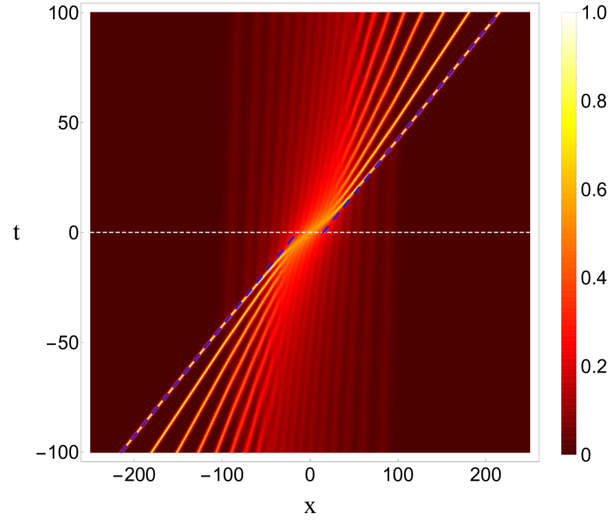
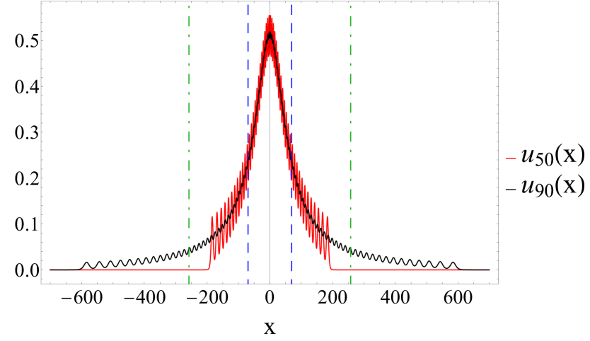
In the existing literature, most of researchers consider the limit of a small density which corresponds to the “rarefied” gas, when solitons interact in some sense weakly, and when approximate approaches can be efficient. In the present work we are not confined by the assumption of a small density of solitons. Quite the opposite, we consider the extreme soliton superposition, which occurs in synchronous soliton collisions, when the reference locations of all the solitons at coincide with the coordinate origin. This property can be formalized through the following symmetry condition, ; it is fulfilled when all the parameters in (3) are put equal to zero: , . An example of such an interaction is shown in Fig. 1.
In what follows, the soliton amplitudes are set decaying exponentially, so that they form a geometric series with the ratio :
| (6) |
Within the KdV framework this choice is in fact rather generic as it corresponds to the distribution of eigenvalues of the scattering problem (represented by the stationary Schrödinger equation) for a parabolic potential, which may serve as a first approximation to any hump-like disturbance.
In the following Secs. III–V the statistical moments of synchronously interacting solitons are examined within the KdV framework. The applicability of the obtained results to a much broader class of equations is discussed in Sec. VI. We relate the fields of focused solitons to the states of the critical density in Sec. VII. Some final conclusions and perspectives are given in Sec. VIII.
III Quasi-stationary states of interacting solitons
The following integrals will be used to measure the statistical moments, similar to Ref. 10:
| (7) |
The choice of the soliton amplitude series (6) ensures that the asymptotic values remain finite for any when .
The use of an ultra-high-precision procedure made it possible to compute the exact -soliton solutions (3) and to calculate the statistical moments (7) for them, when is large, see details in Ref. 12. We found that the moments and , which characterize the wave field asymmetry and kurtosis respectively, decrease in all situations when KdV solitons interact. This observation is in line with the limit of a two-soliton interaction [10] and with the direct numerical simulations of rarefied soliton gases (see e.g. Refs. 6, 13). Representative examples of the evolution of and are given in Fig. 2 for two choices of the parameter and different numbers of interacting solitons . It follows from the figures that the curves converge to some limiting ones when . For the values of closer to the convergence occurs at larger numbers .
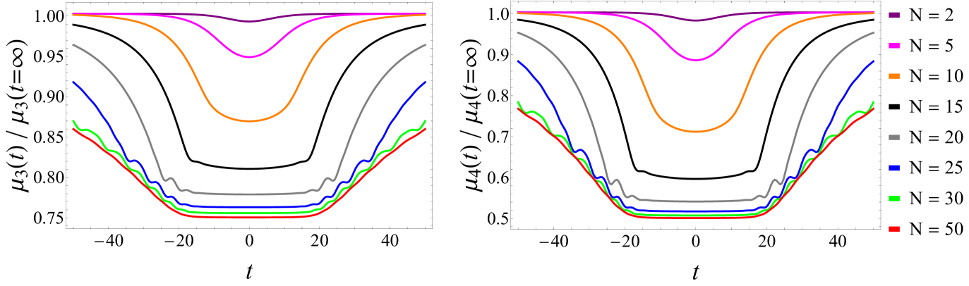
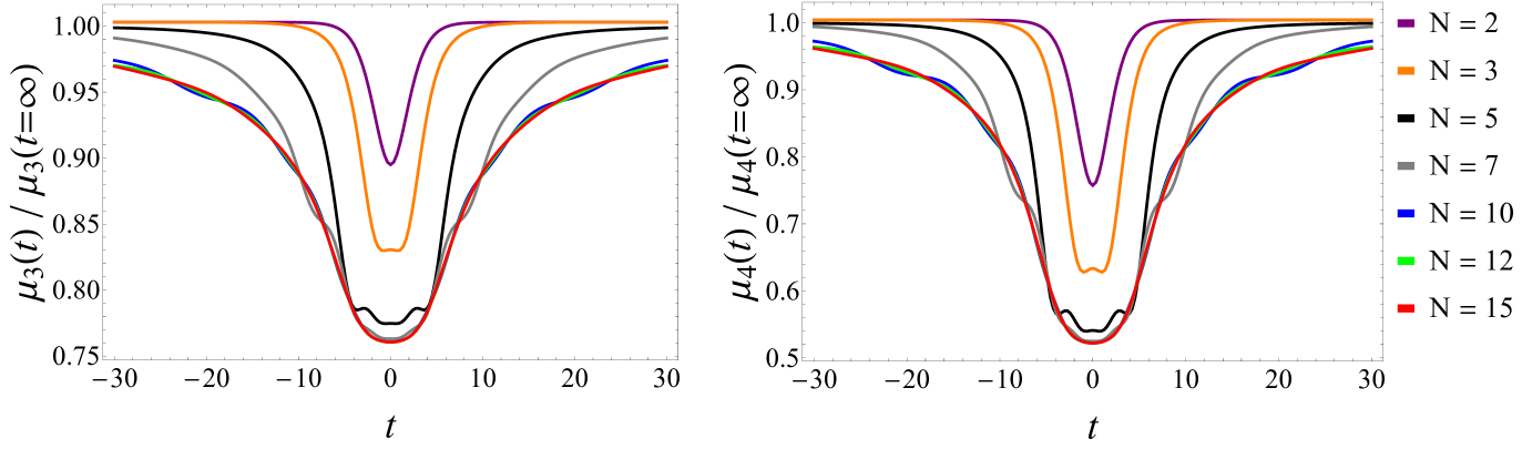
When is sufficiently close to , and is large, the statistical moments remain approximately constant within long time spans, when the solitons are located most densely. This effect is readily seen in the upper panels in Fig. 2 () for , but vanishes for smaller numbers or for significantly larger values of (see the bottom panel in Fig. 2 for ). When is large, the soliton amplitudes in the sequence (6) decay quickly, so that apparently only a few of the largest solitons play a role. Obviously, the observation of “plateaux” in the dependencies , should mean some degeneracy of the soliton state, which we explore below.
IV Smoothing of the wave field in the focusing area
It is well-known that the integrability property of the KdV equation is deeply related to the existence of an infinite series of conserved quantities ,
| (8) |
Hereafter we will use the densities in the form given in Ref. 14. The two first statistical moments and are proportional to the integrals and , and thus do not change in time, while the higher-order statistical moments may vary.
The third conservation integral may be presented in the form
| (9) |
With the use of the asymptotic solution (4), the terms in (9) can be explicitly computed for ,
| (10) |
and then
| (11) |
It was noted in Ref. 10 that since and are strictly positive quantities, the decrease of in the course of the collision leads to the decrease of the second integral, . This should correspond to “smoothing” of the solution in some sense. According to (11), the minimal possible value of , is achieved when totally vanishes. Note that this limit well agrees with the minimum values of observed in Fig. 2 (left column).
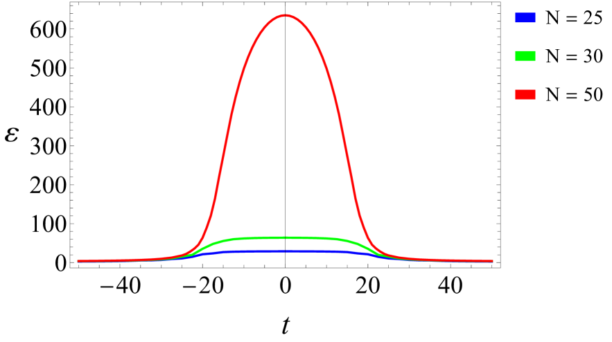
In order to elucidate the nature of the “smoothing” of the wave field, it is instructive to introduce the similarity parameter (the so-called Ursell number), which estimates the ratio of the nonlinear term versus the term of the wave dispersion in the evolution equation (2) for a given solution at a given instant of time. Then the conservation integrals (8) may be presented in the form
| (12) |
see Ref. 15. In these notations, the “smoothing” should correspond to the occurrence of very large values of (in other words, the small-dispersion limit) at . From this, we obtain the estimate for , and then the general formula for any integer assuming :
| (13) |
To obtain the final expression in (13), the integrals and should be calculated for the asymptotic solution (4):
| (14) | |||
| (15) |
The integrals for a single soliton may be found in Ref. 15.
In Fig. 3 the evolution of the Ursell number for the case is shown for different . The Ursell number is calculated using the integral estimator . This quantity has the value for free solitons of any amplitude. One can see from the figure that indeed, the values of become very large when the solitons interact. They further grow if increases. A large number of solitons with close velocities leads to a long time of interaction, what explains the appearance of plateaux in the dependencies and in Fig. 2 (top). For the parameter increases considerably as well, but due to a shorter time of interaction a quasi-stationary behavior of the statistical moments is not observed (Fig. 2, bottom).
One can easily check that the relation (13) aligns with constant moments and , and provides the limiting values and for the drops of the third and fourth moments, which agree with the numerical solutions shown in Fig. 2. It follows from the figure, that the estimates (13) are applicable to long time spans when the solitons focus, if is close to and . According to (13), statistical moments of any order decrease when KdV solitons interact, and this effect becomes stronger for higher moments. We have checked numerically up to the order that the estimate (13) is remarkably accurate, see Table 1.
Examples of the numerical solutions for close to and different finite number of solitons are shown in Fig. 4 for the instant . When grows, the wave smoothing becomes apparent through a decrease in local maxima and an increase in the amplitude of the solution within the valleys between the humps. Accounting for a greater number of solitons in the series (6) leads to further smoothing of the solution and modification of its peripheral part. Presumably, in the limit of a large number of solitons with amplitudes distributed according to the geometric progression they focus into a visually one-hump profile for any . A similar effect in reconstructing a box potential by solitons of the nonlinear Schrödinger equation was found in Ref. 16.
| analytical estimate | deviation, KdV | deviation, mKdV | |
|---|---|---|---|
| 0.08% | 0.36% | ||
| 0.22% | 0.58% | ||
| 0.42% | 0.86% | ||
| 0.72 % | 1.17% | ||
| 1.1% | 1.67% |
V Representative analytical solution
There is a well-known particular shape of the initial perturbation which gives purely discrete spectrum of the associated scattering problem for the KdV equation [17]:
| (16) |
Its evolution leads to the emergence of solitons with zero dispersive tail. The spectral parameters are given by the series
| (17) |
which yields the following relation between soliton amplitudes,
| (18) |
Thus, it is close to the sequence (6) with the ratio , when is large and the soliton sequence numbers are small (i.e., for the tallest solitons).
For the initial-value problem specified by (16), the ratio for an arbitrary -th statistical moment can be evaluated in a few steps using the asymptotic solution (4) and assuming that the number of solitons is large:
| (19) |
Thus, we obtain exactly the same result (13) provided by the qualitative description in the previous section.
VI Broader generality of the result
Since the formulae (14) and (15) are general, the obtained result (13) is valid for any distribution of the soliton amplitudes, as soon as the solution does not change the sign and the similarity parameter is large; the considered example of a perturbation (16) supports this conclusion. This dynamic scenario may be considered as a particular realization of a dense soliton gas. The discovered statistical property of ensembles of a large number of unipolar solitons actually has a much broader application beyond the KdV framework. Below we give a few examples of this fact.
First, the relation (13) is applicable to all members of the hierarchy of integrable KdV equations with the scattering problem represented by the stationary Schrödinger equation. Indeed, in this case the -soliton solutions may be constructed using the same Darboux transformation [8]. The difference will be in the time-dependence of solitons only (i.e., other expressions for the soliton velocity ), but this difference vanishes at the focusing moment and has no effect on the statistical moments when the solitons separate at . Consequently, the moments and will have exactly the same values as before. The obtained results obviously can be extended to higher dimensions, such as the Kadomtsev – Petviashvili equation.
The focusing modified Korteweg – de Vries (mKdV) equation
| (20) |
has a different from the classic KdV associated scattering problem, but as other integrable systems, possesses an infinite number of conserved quantities , . Soliton solutions of the mKdV equation have two branches of solitons on a zero background which differ in a sign (polarity).
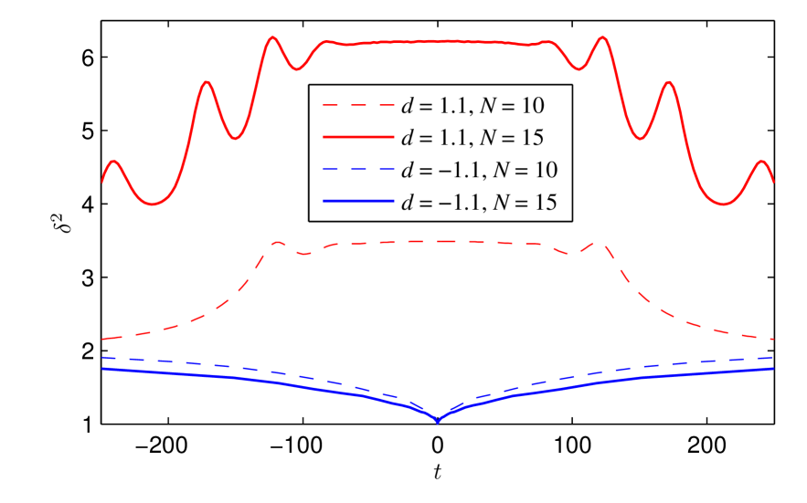
If the similarity parameter of the mKdV equation , which may be estimated as becomes large (i.e., the small-dispersion regime takes place), then to the leading order the conservation integrals are proportional to the statistical moments, , . The evolution of the parameter in two examples of interaction of mKdV solitons of the same sign is shown in Fig. 5 with red curves. A similar approach based on the Darboux transform is used to construct -soliton solutions of the mKdV equation, see Ref. 4. The soliton amplitudes are specified according to the same law (6) as in the case of the KdV equation. During interaction, the parameter greatly exceeds the value which corresponds to free soliton solutions, if is close to and is sufficiently large.
Therefore, when the nonlinear term in the equation dominates over the term of dispersion, one can straightforwardly estimate the relative decrease of the statistical moments with even orders . Remarkably, these estimates exactly coincide with the ones for the KdV equation (13). Even more, we have checked numerically that odd orders of the statistical moments satisfy the relation (13) too,
| (21) |
Note the perfect agreement between numerical results and the analytical estimates in Table 1.
In fact, equations (2) and (20) are related by the complex Miura transformation
| (22) |
which maps solutions of the mKdV equation to complex-valued solutions of the complex Korteweg – de Vries (cKdV) equation on which has the form identical to (2) (see e.g. Ref. 18).
The balance of terms in the Miura transformation is controlled by the similarity parameter of the mKdV equation, which quantifies the contribution of the nonlinear term in (22) with respect to the imaginary term of dispersion, so that the real part effectively dominates at the focal point . That provides an estimate . At asymptotically large times solitons of the mKdV equation are mapped to , where real is now the spectral parameter of the scattering problem for the mKdV equation. The expression for coincides with the single soliton solution for the KdV equation (see (4) putting ) except for the imaginary phase shift. The imaginary phase shift does not influence the integrals , they remain real-valued. Therefore, one can straightforwardly obtain that . As a result, the statistical moments for the solution of the complex KdV equation, , may be also expressed through the ratio (21):
| (23) |
VII Localization size of the focused soliton train
During the intervals of almost constant reduced statistical moments the interacting KdV solitons are located most closely and are characterized by large Ursell numbers. It seems reasonable to associate these extreme quasi-stationary states with the situation of the critical soliton density.
Importantly, the focused solitons represent essentially non-uniform in space wave fields, thus the adopted formulas, which relate the averaging in the physical space to the averaging in the spectral domain and eventually lead to the formula (5), become questionable. One can straightforwardly check that the definition (5) for the soliton amplitudes taken in the form of a geometric series (6) yield the values proportional to , hence the quantity grows infinitely if . Bearing this in mind, let us consider the quantity which has the meaning of some characteristic size, assuming that is still determined by (5). For the exponential distribution of the soliton amplitudes (6) the values of are finite:
| (24) |
To estimate the actual size of the spatial domain occupied by the solution at , we consider the coordinate shift which solitons experience when pass through all the other solitons in the train (see Fig. 1). The shift for the -th soliton, , is given by the classic formula
| (25) |
Due to the factor , the shift of small-amplitude solitons is not bounded from above when . On the other hand, the shift of the largest soliton is the least affected by an addition of small-amplitude solitons. Therefore we represent the characteristic size of the focused solution through the shift of the largest soliton, . The blue dashed lines in Fig. 1 correspond to the plots for and for . They follow the paths of the largest solitons when and confine the interval when cross the axis . For the soliton amplitudes distributed according to (6), this quantity can be calculated assuming is large and is close to ,
| (26) |
The estimated size of the focused wave has the same dependence on the governing parameter as the critical size (24), with the proportionality coefficient .
For the shape (16) the characteristic size of the focused solution can be estimated using (25) as . One can also calculate the critical width for this example directly using the formula for the critical density (5) and the distribution of soliton amplitudes according to (17), ; so for this case .
For the examples of multisoliton solutions and shown in Fig. 4 the characteristic sizes are , and , correspondingly. It may be seen from the figure that the scales and are in good compliance with the visible size of the focused wave train. One may speculate that the extreme compression of solitons which occurs in the considered scenarios of soliton collisions corresponds to the states with the minimum allowed (critical) size of the soliton ensemble. The scale underestimates the actual visible size of the focused solution, and can be used as the estimate from below.
VIII Conclusion
In this work we present a general idea that dense ensembles of solitons of the same sign (say, KdV-type solitons) can be considered as the strongly-nonlinear / small-dispersion wave states, what allows to express the statistical moments in terms of the spectral parameters of the associated scattering problem. Synchronous collisions of many solitons with slowly decaying amplitudes have been considered as a particular case when the dense soliton state can occur. We made a qualitative assumption (without a rigorous justification) on the relation between the critical soliton density and the minimal size of the focused solitons, which shows a reasonable agreement.
A broad applicability of the employed concept to other integrable systems is anticipated, we have given several confirming examples. Since weakly non-integrable systems typically inherit the soliton dynamics with little alteration (see e.g. Ref. 11), we may expect that the obtained results can be applied to non-integrable generalizations of the equations too.
At the same time, the approach apparently does not allow one to estimate the statistical moments in the case of simultaneous collisions of solitons with different signs, when they can cause wave amplification, which is not limited from above with an increase in the number of solitons [3, 4]. It follows from the direct numerical calculations that in the course of collision of mKdV solitons with alternating signs, the similarity parameter associated with the integral ratio, , decreases from the value which corresponds to free soliton solutions, but not much. It never falls below the value , see the blue curves in Fig. 5. Hence, a discrimination of terms which constitute the conservation integrals does not occur. Since phases of soliton solutions are not affected by their signs, the synchronous collision of solitons with alternating polarities formally leads to the creation of an equally dense soliton state, as in the case when solitons have the same signs. However, the statistical moments of the focusing solitons of different signs change rapidly, in contrast to the case of unipolar solitons.
In that way, a counterintuitive situation takes place, when interacting solitons of the same sign produce a strongly nonlinear state in terms of the similarity parameter, but which does not contain high waves. At the same time, the collision of solitons of different signs may cause extremely high wave amplitudes but is characterized by a relatively small ratio of nonlinearity versus dispersion.
Author’s contributions
All authors contributed equally to this work.
Acknowledgements.
The authors are grateful to M.V. Pavlov and E.N. Pelinovsky for valuable stimulative discussions. The work on Sec. VI was supported by the Foundation for the Advancement of Theoretical Physics and Mathematics “BASIS” No 22-1-2-42. The remaining sections were supported by the RSF grant No 19-12-00253. The authors are grateful to the anonymous referee for valuable comments.Data Availability Statement
Data available on request from the authors.
References
- Zakharov [1971] V. E. Zakharov, “Kinetic equation for solitons,” JETTP 33, 538–541 (1971).
- El and Kamchatnov [2005] G. A. El and A. M. Kamchatnov, “Kinetic equation for a dense soliton gas,” Phys. Rev. Lett. 95, 204101 (2005).
- Slunyaev and Pelinovsky [2016] A. V. Slunyaev and E. N. Pelinovsky, “The role of multiple soliton interactions in generation of rogue waves: the mKdV framework,” Phys. Rev. Lett. 117, 214501 (2016).
- Slunyaev [2019] A. Slunyaev, “On the optimal focusing of solitons and breathers in long wave models,” Stud. Appl. Math. 142, 385–413 (2019).
- El [2016] G. A. El, “Critical density of a soliton gas,” Chaos 26, 023105 (2016).
- Pelinovsky and Shurgalina [2017] E. Pelinovsky and E. Shurgalina, “Challenges in complexity: Dynamics, patterns, cognition,” (Springer, 2017) Chap. KDV soliton gas: interactions and turbulence, pp. 295–306.
- Soto-Crespo, Devine, and Akhmediev [2016] J. M. Soto-Crespo, N. Devine, and N. Akhmediev, “Integrable turbulence and rogue waves: breathers or solitons?” Phys. Rev. Lett. 116, 103901 (2016).
- Matveev and Salle [1991] V. B. Matveev and M. A. Salle, Darboux transformations and solitons (Springer-Verlag, 1991).
- Gardner et al. [1974] C. S. Gardner, J. M. Greene, M. D. Kruskal, and R. M. Miura, “Korteweg – de Vries equation and generalizations. VI. Methods for exact solution,” Commun. Pure Appl. Math. 27, 97–133 (1974).
- Pelinovsky et al. [2013] E. Pelinovsky, E. Shurgalina, A. Sergeeva, T. Talipova, G. El, and R. Grimshaw, “Two-soliton interaction as an elementary act of soliton turbulence in integrable systems,” Phys. Lett. A 377, 272–275 (2013).
- Dutykh and Pelinovsky [2014] D. Dutykh and E. Pelinovsky, “Numerical simulation of a solitonic gas in KdV and KdV-BBM equations,” Phys. Lett. A 378, 3102–3110 (2014).
- Tarasova and Slunyaev [2022] T. Tarasova and A. Slunyaev, “Properties of synchronous collisions of solitons in the Korteweg – de Vries equation,” (2022), arXiv: 2208.04762 .
- [13] E. D. (Shurgalina), “Numerical modeling of soliton turbulence within the focusing Gardner equation: Rogue wave emergence,” Phys. D 399, 35–41 (2019).
- Miura, Gardner, and Kruskal [1968] R. Miura, C. Gardner, and M. Kruskal, “Korteweg-de Vries equation and generalizations. II. Existence of conservation laws and constants of motion,” Journal of Mathematical Physics 9, 1204 (1968).
- Karpman [1975] V. Karpman, Non-Linear Waves in Dispersive Media (Pergamon, 1975).
- Gelash et al. [2021] A. Gelash, D. Agafontsev, P. Suret, and S. Randoux, “Solitonic model of the condensate,” Phys. Rev. E 104, 044213 (2021).
- G.L. Lamb [1980] J. G.L. Lamb, Elements of soliton theory (Wiley, 1980).
- Sun, Yuan, and Zhang [2014] Y.-Y. Sun, J.-M. Yuan, and D.-J. Zhang, “Solutions to the complex Korteweg – de Vries equation: blow-up solutions and non-singular solutions,” Commun. Theor. Phys. 61, 415–422 (2014).