Statistical Study of Coronal Mass Ejection Source Locations: II. Role of Active Regions in CME Production
Abstract
This is the second paper of the statistical study of coronal mass ejection (CME) source locations, in which the relationship between CMEs and active regions (ARs) is statistically studied on the basis of the information of CME source locations and the ARs automatically extracted from magnetic synoptic charts of Michelson Doppler Imager (MDI) during 1997 – 1998. Totally, 224 CMEs with a known location and 108 MDI ARs are included in our sample. It is found that about 63% of the CMEs are related with ARs, at least about 53% of the ARs produced one or more CMEs, and particularly about 14% of ARs are CME-rich (3 or more CMEs were generated) during one transit across the visible disk. Several issues are then tried to clarify: whether or not the CMEs originating from ARs are distinct from others, whether or not the CME kinematics depend on AR properties, and whether or not the CME productivity depends on AR properties. The statistical results suggest that (1) there is no evident difference between AR-related and non-AR-related CMEs in terms of CME speed, acceleration and width, (2) the size, strength and complexity of ARs do little with the kinematic properties of CMEs, but have significant effects on the CME productivity, and (3) the sunspots in all the most productive ARs at least belong to type, whereas 90% of those in CME-less ARs are or type only. A detailed analysis on CME-rich ARs further reveals that (1) the distribution of the waiting time of same-AR CMEs, consists of two parts with a separation at about 15 hours, which implies that the CMEs with a waiting time shorter than 15 hours are probably truly physical related, and (2) an AR tends to produce such related same-AR CMEs at a pace of 8 hours, but cannot produce two or more fast CMEs ( km s-1) within a time interval of 15 hours. This interesting phenomenon is particularly discussed.
1 Introduction
Coronal mass ejections (CMEs) are one of the most violent explosive phenomena in the solar atmosphere, and active regions (ARs) are thought to be the most efficient producer of CMEs because free energy tends to accumulate there. However, different ARs may have different capability of generating CMEs, and CMEs may not be necessary to take place in ARs. These two facts leave the relationship between CMEs and ARs still an unresolved issue.
Previous studies have shed light on the AR’s capability of producing (strong) CMEs. Through examining 117 ARs, Canfield et al. [1999] found that ARs are more likely to be eruptive if they are either sigmoidal or large. Guo et al. [2007] investigated 55 flare-CME productive ARs and found that fast CMEs tended to initiate in ARs with large magnetic flux or long lengths of main polarity inversion lines (PILs). Through investigating 57 fastest CMEs with speed larger than 1500 km s-1 from 1996 June to 2007 January as well as 1143 ARs recognized from magnetic synoptic charts obtained by Michelson Doppler Imager (MDI) on board Solar and Heliospheric Observatory (SOHO), Wang and Zhang [2008] found that there was a general trend that a larger, stronger, and more complex AR was more likely to produce a faster CME. A systematical study was also performed by Falconer et al. [2002, 2006, 2008, 2009] in their series papers. They found that the CME productivity of a bipolar AR depended on the global nonpotentiality of the AR’s magnetic field. Furthermore, Yeates et al. [2010] identified and investigated 98 front-side CMEs during 1999 May 13 – September 26, compared their source regions with the simulation results of coronal magnetic field evolution, and found that the strong gradient of the radial component of magnetic field at photosphere, that usually appears in ARs, may be a good indicator of CME-productive regions.
Similar dependence on AR free energy can be found in many studies of the flare productivity of ARs [e.g., Sammis et al., 2000; Leka and Barnes, 2003, 2007; Maeshiro et al., 2005; Jing et al., 2006; Ternullo et al., 2006; Schrijver, 2007; Georgoulis and Rust, 2007; Su et al., 2007]. Although flares are also a violent explosive phenomenon in the solar atmosphere, they are different from CMEs. Flares can be classified as either confined ones or eruptive ones according to whether or not they are associated with CMEs [e.g., Svestka and Cliver, 1992; Wang and Zhang, 2007; Schrijver, 2009]. Thus the statistical results obtained for flares and CMEs are similar but not the same. An example for the difference between flares and CMEs can be seen from the flare and CME productivities of an AR-complex reported by Akiyama et al. [2007], in which two adjacent flare-productive ARs have much different levels of CME association. Moreover, they found that for the CME-rich AR, the average waiting time of flares is much longer than that for the CME-poor AR. We know that sufficient free energy is a necessary condition for an AR to be eruptive [e.g., Priest and Forbes, 2002; Régnier and Priest, 2007]. Since both flares and CMEs consume the free energy, flares and CMEs sometimes may work as two competing processes. From this perspective, to understand AR’s ability of producing CMEs is different from that producing flares, and thus becomes a more complicated issue.
On the other hand, the association of CMEs with ARs has also been widely studied. Through examining 32 CMEs whose source regions were located on the solar disk and well observed in EIT 195 Å from 1996 January through 1998 May, Subramanian and Dere [2001] found that about 84% CMEs were associated with ARs. Zhou et al. [2003] studied 197 front-side halo CMEs (angular width ) from 1997 to 2001 and found that there were about 79% front-side halo CMEs originating from ARs. It has been suggested for a long time that there might be two distinct types of CMEs [e.g., MacQueen and Fisher, 1983; St. Cyr et al., 1999; Sheeley, Jr. et al., 1999; Delannée et al., 2000; Andrews and Howard, 2001; Moon et al., 2002]. One type of CMEs is associated with flares and usually originates from ARs; they have a constant or decreasing speed in the outer corona, implying an impulsive acceleration process in the inner corona. The other type of CMEs is often associated with quiescent filament-eruptions; their speeds increase with a nearly constant acceleration, implying a gradual acceleration process. However, several more recent statistical studies reached an opposite conclusion that there is no two distinct types of CMEs [e.g., Yurchyshyn et al., 2005; Vršnak et al., 2005; Chen et al., 2006]. Counter cases can be often observed. For example, Feynman and Ruzmaikin [2004] presented a quiescent filament-associated CME, which reached an extremely fast speed in the corona. Similar cases can be found in the paper by Wang and Zhang [2008], e.g., the CMEs occurring on 1998 April 20 and 2002 May 22. Thus, the issue whether or not there are two distinct types of CMEs and the role of ARs in this issue are worth to be clarified.
Apparently, further studies are needed to fully understand the role of ARs in producing CMEs. What kind of ARs can or cannot produce CMEs? What kind of ARs can frequently produce CMEs? What causes different kinematic properties of CMEs? Any inputs from observations, in particular, results from statistical studies, can be used to constrain theoretical models. In our previous study [Wang et al., 2011, hereafter referred as Paper I], we have manually identified the source locations of all CMEs from 1997 to 1998, and a total of 288 CMEs have been located their source regions on the visible solar disk (refer to http://space.ustc.edu.cn/dreams/cme_sources/). In our another paper by Wang and Zhang [2008], we developed an automatic method to detect and quantitatively characterize ARs from photospheric magnetogram images. Thus, the two works provide us the observational base for investigating the relationship between ARs and CMEs. The paper is organized as follows. In Sec.2, we introduce the data of CMEs and ARs which will be used in this study. Then we present the statistical results of the dependence of CME apparent properties on ARs in Sec.3. The CME productivity of ARs is presented in Sec.4. In Sec.5, we further study those ARs frequently producing CMEs. Finally, summary and conclusions are given in Sec.6 and Sec.7.
2 Data and Method
ARs usually appear as bright patches on the Sun in the EUV wavelengths, and have strong magnetic field. A frequently referred catalog of ARs is compiled by NOAA SWPC111Space Weather Prediction Center, http://www.swpc.noaa.gov/ftpmenu/forecasts/SRS.html, in which several parameters of ARs and the corresponding sunspot groups are given, such as the location, area, classifications, sunspot number, etc. However, the NOAA AR catalog lacks of some key quantitative information of ARs such as magnetic field strength, flux, etc. For this sake, we developed an automatic method in 2008 to extract ARs based on the synoptic charts of photospheric magnetic field from SOHO/MDI; they are called MDI ARs. Through this method, ARs can be recognized and parameterized with a uniform set of criteria, free of personal biases in the identification process. A detailed description of the method and the comparison of MDI ARs with NOAA ARs can be found in Wang and Zhang [2008] and a follow-up paper by Zhang et al. [2010].
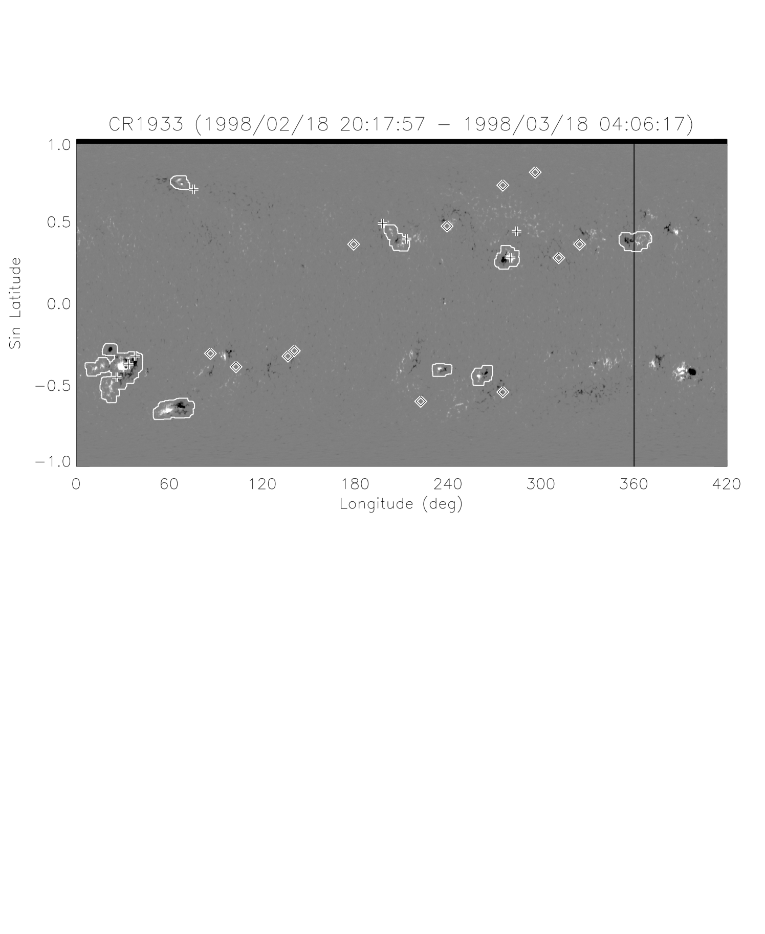
In this paper, we will use the MDI ARs rather than the traditional NOAA ARs to study the role of ARs in producing CMEs. Figure 1 shows the MDI ARs from Carrington rotation 1933, as an example. The plus and diamond symbols marked on the map indicate the locations of AR-related and non-AR-related CMEs, respectively; the Carrington longitude and latitude of these CMEs correspond to the heliographic coordinates of the CME source location at the time observed in EIT.
To determine if a CME is related to an AR and which AR is related to, we first identify the source locations of the CME. As mentioned before, all the LASCO CMEs during 1997 – 1998 had been checked with their source locations, and 288 CMEs were identified as front-side CMEs, namely location identified (LI) CMEs. One can refer to Paper I Section 2 for the detailed process of the identification. Briefly, we manually checked SOHO/EIT movies, and looked for any surface signatures of CMEs, such as flares, dimmings, waves, post-eruption loops, etc. If there was one or several eruption signatures reasonably close to the time and direction of a CME viewed in SOHO/LASCO, the CME is considered as a LI CME, and the center of the surface eruption feature is then chosen as its location.
Then we calculate the spherical surface distances (, in units of degree) between the CME and the boundaries of nearby ARs. If there is at least one AR within a threshold distance , the CME is AR-related (as marked by the pluses in Fig. 1) and the related AR is the one having the shortest distance; otherwise, the CME is non-AR-related (the diamonds in Fig. 1). Considering the error in determination of CME locations and the projection effect for those CMEs close to solar limb, we set for CMEs with and for CMEs with . Here the quantity is the projected distance on the plane-of-sky between the CME location and the solar disk center (see Paper I for details). Meanwhile, for each AR, we classify it as either a CME-less or CME-producing AR, depending on whether a CME is associated with this AR or not. Further, we define an AR as a CME-rich AR, if it produced three or more CMEs.
Compared to a snapshot MDI magnetogram image, a synoptic chart does not show the exact state of the photospheric magnetic field during a CME. However, it has the advantage of reduced projection effect, in particular, for those CMEs far away from the solar disk center. For these CMEs, it is almost impossible to obtain the correct information of photospheric magnetic field surrounding the CME source location, due to the presence of significant projection effect. Further, snapshot magnetograms cannot provide us the magnetic information behind the solar limb. On the other hand, as shown in Paper I there were 56% of CMEs with known source location occurring for . Thus, it is necessary to use MDI synoptic charts for the study of this paper.
| CMEs | ||
|---|---|---|
| AR-related | 141 | 63% |
| Non-AR-related | 83 | 37% |
| Total | 224 | |
| MDI ARs | ||
| CME-less | 51 | 47% |
| CME-producing1 | 57 | 53% |
| CME-rich2 | 15 | 14% |
| Total | 108 | |
1 A CME-producing AR means the AR produced at least one CME during
its passage across the visible disk.
2 A CME-rich AR means the AR produced 3 or more CMEs. Thus CME-rich
ARs are a subset of CME-producing ARs.
Due to the presence of data gaps of SOHO observations, some MDI magnetic synoptic charts are incomplete. The CMEs corresponding to these incomplete synoptic charts are simply excluded in the analysis. Also some LI CMEs with a low confidence level () are removed. Finally, there are in total 224 LI CMEs with MDI synoptic charts available and a total of 108 MDI ARs during the period of study from 1997 – 1998. It is straightforward to obtain that about 63% of LI CMEs are related with ARs, while the rest 37% of LI CMEs are not related with any AR. Meanwhile, about 47% of ARs do not produce a single CME during the period crossing through the visible solar disk. About 53% of ARs produce at least one CME. Particularly, about 14% of ARs produce at least 3 CMEs, thus are CME-rich. The numbers of different types of CMEs and MDI ARs are summarized in Table 1. The fractions of different types of MDI ARs are not accurate, because we are unable to learn the activity of an AR before it rotates to the front-side of the disk and after it rotates to the back-side of disk. Nevertheless, one could assume that the activity level of a particular AR, is similar in the front-side as in the back-side. It is probably true as one will see in Sec.5.2 that the CME productivity of ARs is related with the AR complexity, but not the AR phase.
3 Dependence of CME Apparent Properties on ARs
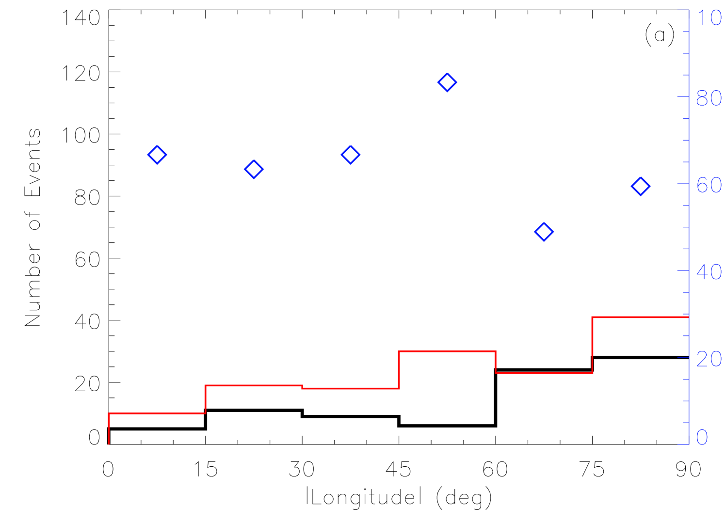
First of all, we make a comparison study of AR-related and non-AR-related CMEs. The association rate of CMEs with ARs is about 63% in this study. The variation of association rate along the absolute value of the heliographic longitude is shown in Figure 2a, in which one can find that there is no significant difference between the limb and on-disk fraction of AR-related CMEs. Thus we can conclude that the associations of limb CMEs with ARs are reliable even though the projection effect is maximized in determining the source location of limb CMEs. Moreover, the fraction of AR-related CMEs is decreasing only slightly for longitude . Since and longitude are closely related for low latitudes (where ARs are located), this justifies the simple criteria used for AR association (see the 4th paragraph of Sec.2). In particular, the sudden increase of from to has not the effect to increase the CME association to ARs for . But there is a significant increase of both numbers of AR-related and non-AR-related CMEs with longitude. This is due to the presence of occulting effect, Thomson scattering effect and projection effect (see Paper I for details).
The value of the association rate, 63%, obtained in this study is smaller than 84% and 79% obtained respectively by Subramanian and Dere [2001] and Zhou et al. [2003]. This difference seems to be caused by the bias in the selection of events. In their studies, only well observed CMEs and/or halo CMEs were investigated, while in this paper, all CMEs are included, no matter whether a CME is halo or narrow, and bright or faint. This difference suggests that there is a significant fraction of CMEs may originate from quiet Sun regions, and these CMEs tend to be weak and/or narrow. Figure 2b presents the distribution of the apparent angular width for AR-related and non-AR-related CMEs with , in which the projection effect is minimized. A weak difference could be found between the two sets of CMEs that the non-AR-related CMEs are slightly narrower than AR-related CMEs.
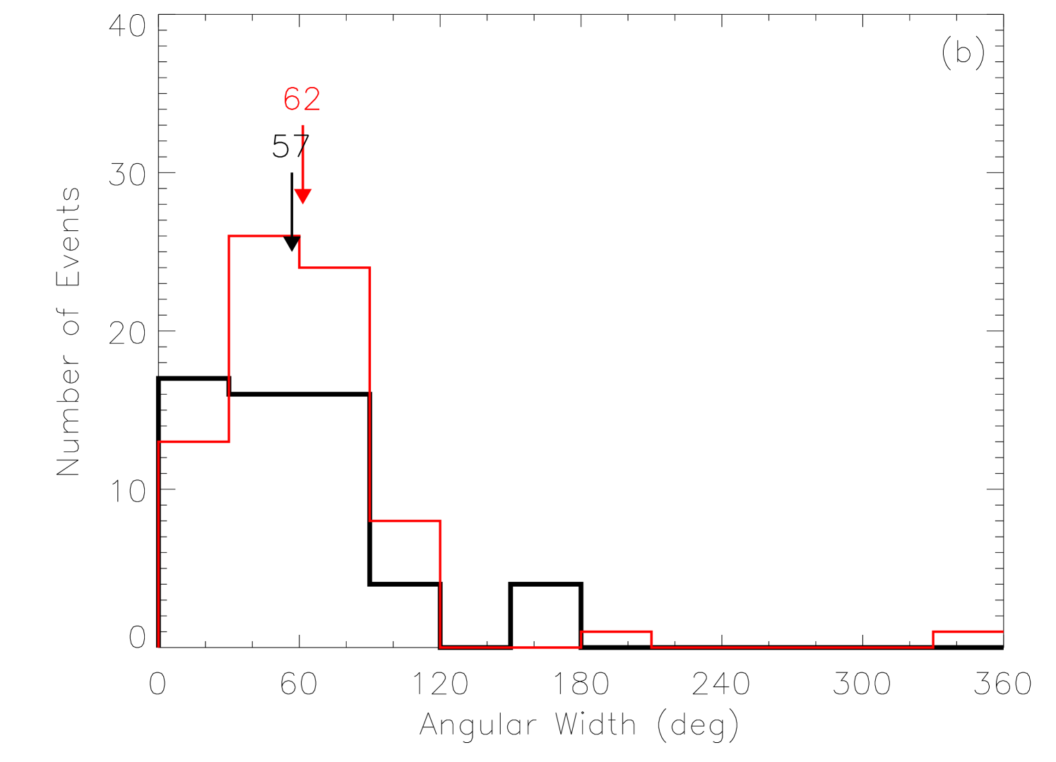
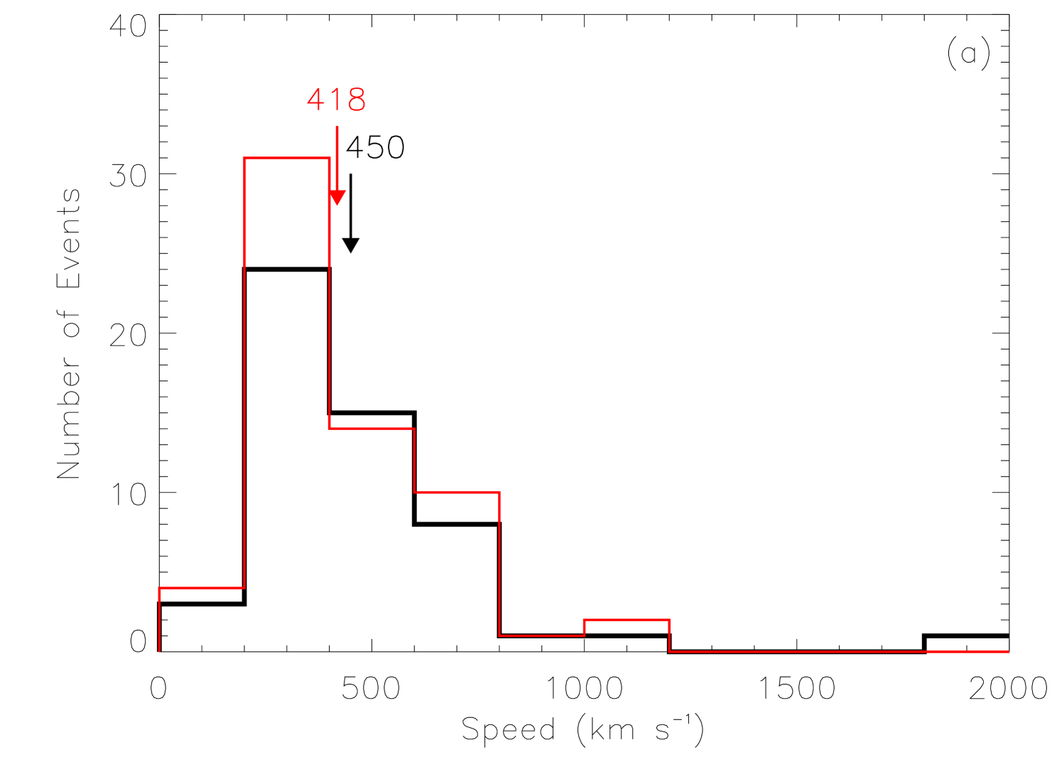
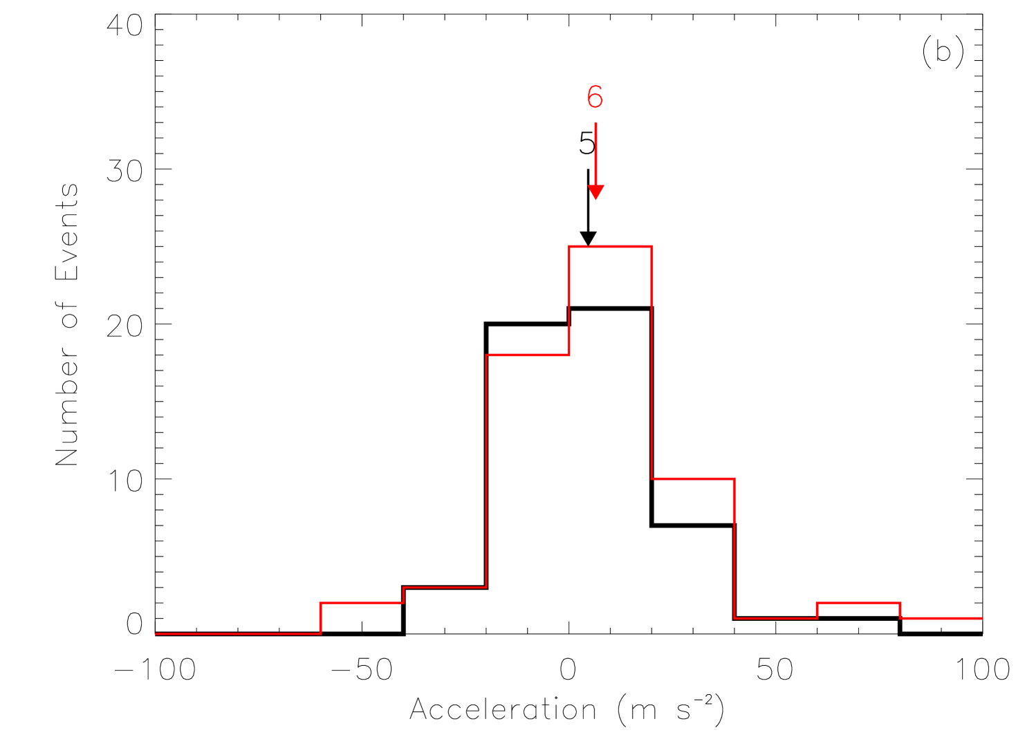
As mentioned in the Introduction, there perhaps exist two types of CMEs in terms of their kinematic behavior. One type of CMEs is impulsive and often associated with flares, and the other type of CMEs is gradual and often associated with prominences. The former type of CMEs usually has a faster speed and smaller acceleration in the outer corona than the latter [e.g., Sheeley, Jr. et al., 1999]. Here, we compare the AR-related and non-AR-related CMEs, in order to check whether or not there are two different types of CMEs caused by difference types of source regions.
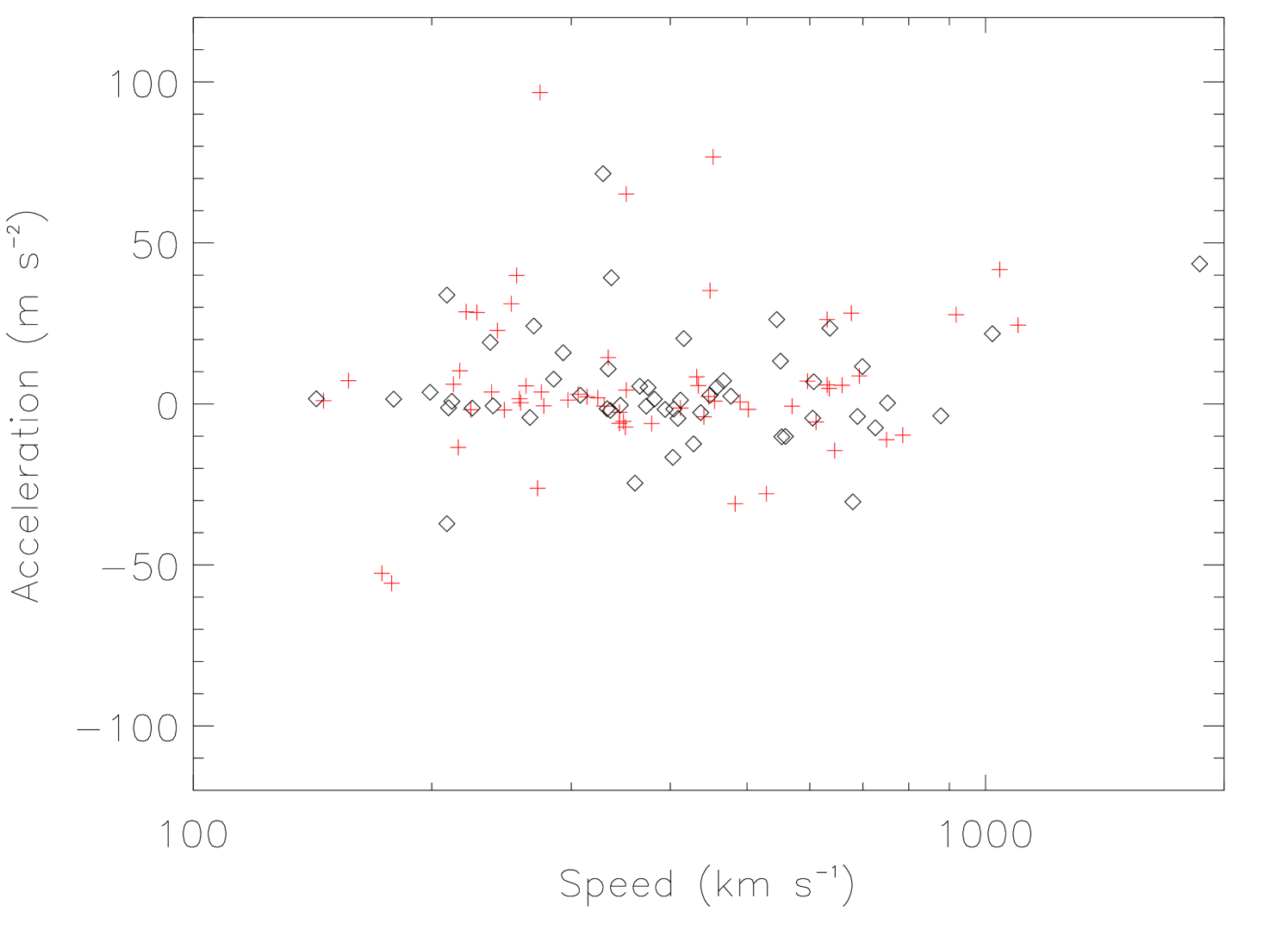
Figure 3 shows the distributions of apparent speed and acceleration of the AR-related and non-AR-related CMEs. To minimize the bias of the projection effect, only limb CMEs (i.e., and width ) with effectively measured speed and acceleration are considered here. This selection results in 62 AR-related CMEs and 53 non-AR-related CMEs. As shown in the figure, the distributions of the two sets of CMEs are quite similar. Both AR-related and non-AR-related CMEs can reach a very fast speed and/or a large acceleration/deceleration. Further, we show the scattering plot between CME speeds and accelerations for the two sets of CMEs in Figure 4. There is no evident difference between the two sets of CMEs. These results are consistent with the studies by Yurchyshyn et al. [2005]; Vršnak et al. [2005]; Chen et al. [2006], who applied different classifications and also found no evidence supporting the existence of two distinct types of CMEs.
Second, we investigate if the AR properties may have an influence on the CMEs kinematic properties. We again consider only limb CMEs, to reduce the projection effect; full halo CMEs and those CME without speed measured are removed from our sample. There are 71 AR-related limb CMEs originating from 42 ARs. Since some ARs produced more than one CME, the CME number is more than the AR number. For those multiple-CME-producing ARs, we use the fastest CME as the representative of the AR in the following analysis, because the fastest CME may reflect the capability of an AR producing a strong eruption.
For each MDI AR, our automatic AR-detection method can extract at least 12 parameters, including that of areas, magnetic fluxes, magnetic field strength, AR shape and PILs. We choose the following parameters for further analysis: total area (), total magnetic flux (), total length of PILs () and number of PILs ()222In our algorithm of recognizing AR and extracting parameters, some pixels in an AR with weak magnetic field are removed due to the preset threshold [refer to Wang and Zhang, 2008]. The present threshold perhaps may also remove some pixels around PILs so that positive and negative polarities may be no longer apparently adjacent and PILs can not be extracted. Actually, this treatment may keep main PILs and ignore minor PILs. Thus, ARs without PILs do exist in our sample, but they are not unipolar regions.. These parameters had proved to have influence on AR’s capability of producing extremely fast CMEs [see Wang and Zhang, 2008].
| Speed | 453.81 | -44.66 | -20.78 | 68.31 | 2.23 | 0.22 |
| Width | 58.23 | -39.09 | 35.62 | 15.97 | -11.49 | 0.45 |
∗ Column are the coefficients in Eq.1. The last column gives the correlation coefficients between the observed values and the fitting results from the linear regression analysis. The second and third row is for the CME apparent speed and width, respectively.
Figure 5 presents the dependence of CME speeds and angular widths on four AR parameters: , , and . In each panel, the plus symbols mark the average value and the standard deviation of the data points within the range indicated by the horizontal bars. Apparently, no evident correlation can be found for these parameters. We further look into the possibility that CME speed and width may be correlated with the combination of the AR parameters. Thus, we apply linear regression analysis on the data. The following function is fitted:
| (1) | |||||
where is the CME speed or angular width, means the average value of quantity , and are the coefficients to be fitted.
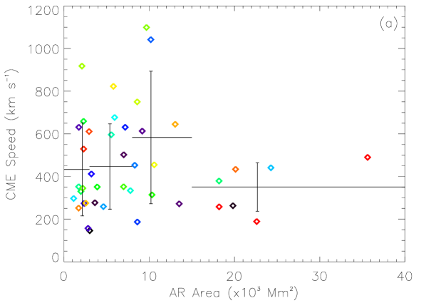
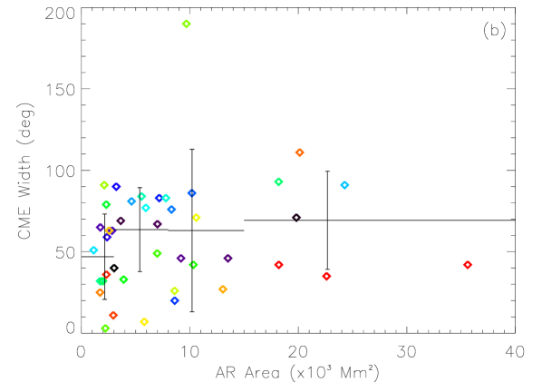
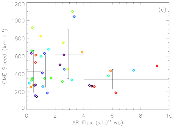
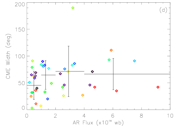
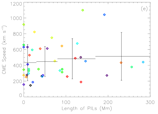
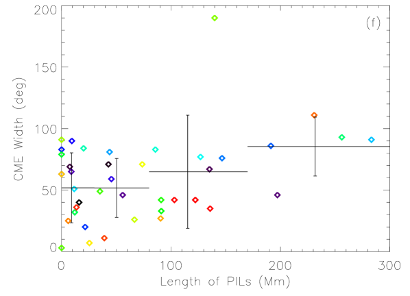
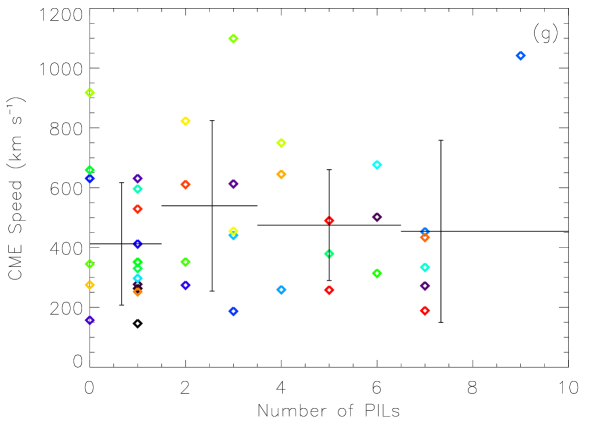
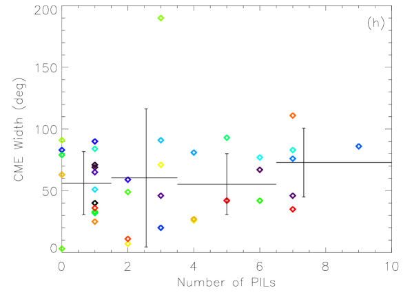
Figure 6 shows the fitting results, and the obtained coefficients, and correlation coefficient, , are listed in Table 2. For CME speed, the value of is only 0.22, suggesting that there is almost no correlation between CME speed and the AR parameters we chose. In our previous study [Wang and Zhang, 2008], we reached a conclusion that an AR with larger area, stronger magnetic field and more complex morphology has a higher possibility of producing extremely fast CMEs (speed km s-1). Our statistical result in this paper indicates that the same conclusion cannot be extended to CMEs with slower speed. For CME width, a weak correlation () can be seen in Figure 6(b). It means that the size, strength and complexity of ARs may have an impact on the size of produced CMEs. Moreover, from Table 2, we find that the coefficients, and , are most significant, suggesting that AR area and total magnetic flux are more important factors in determining the CME size.


4 CME Productivity of ARs
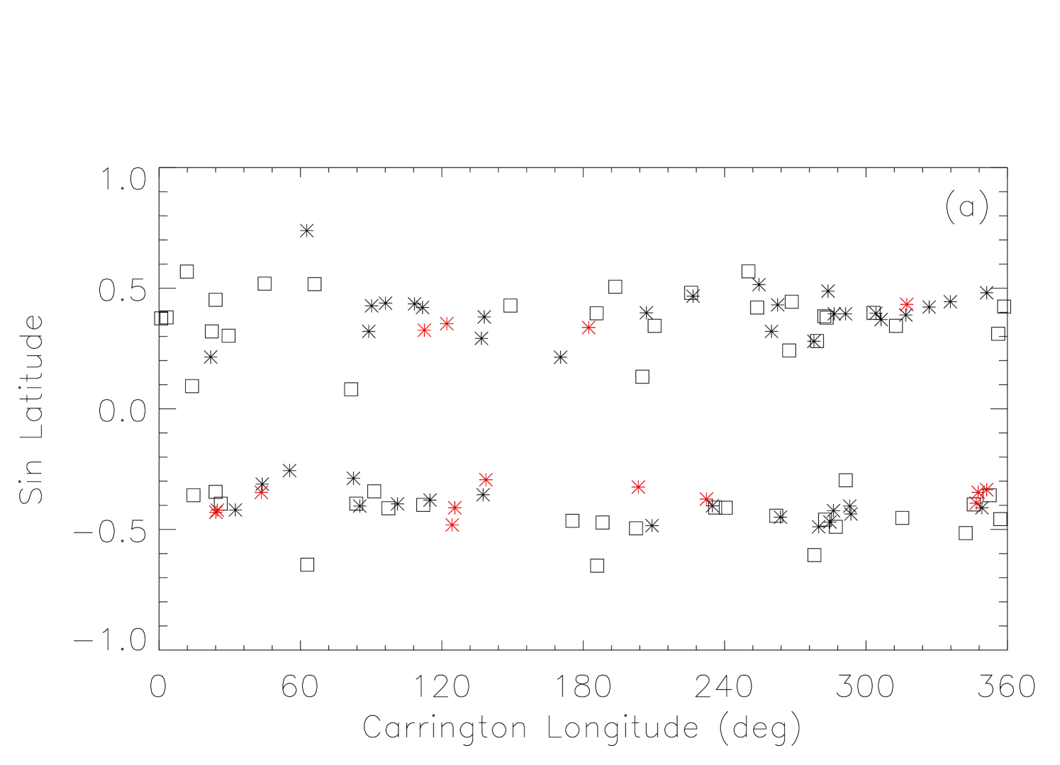
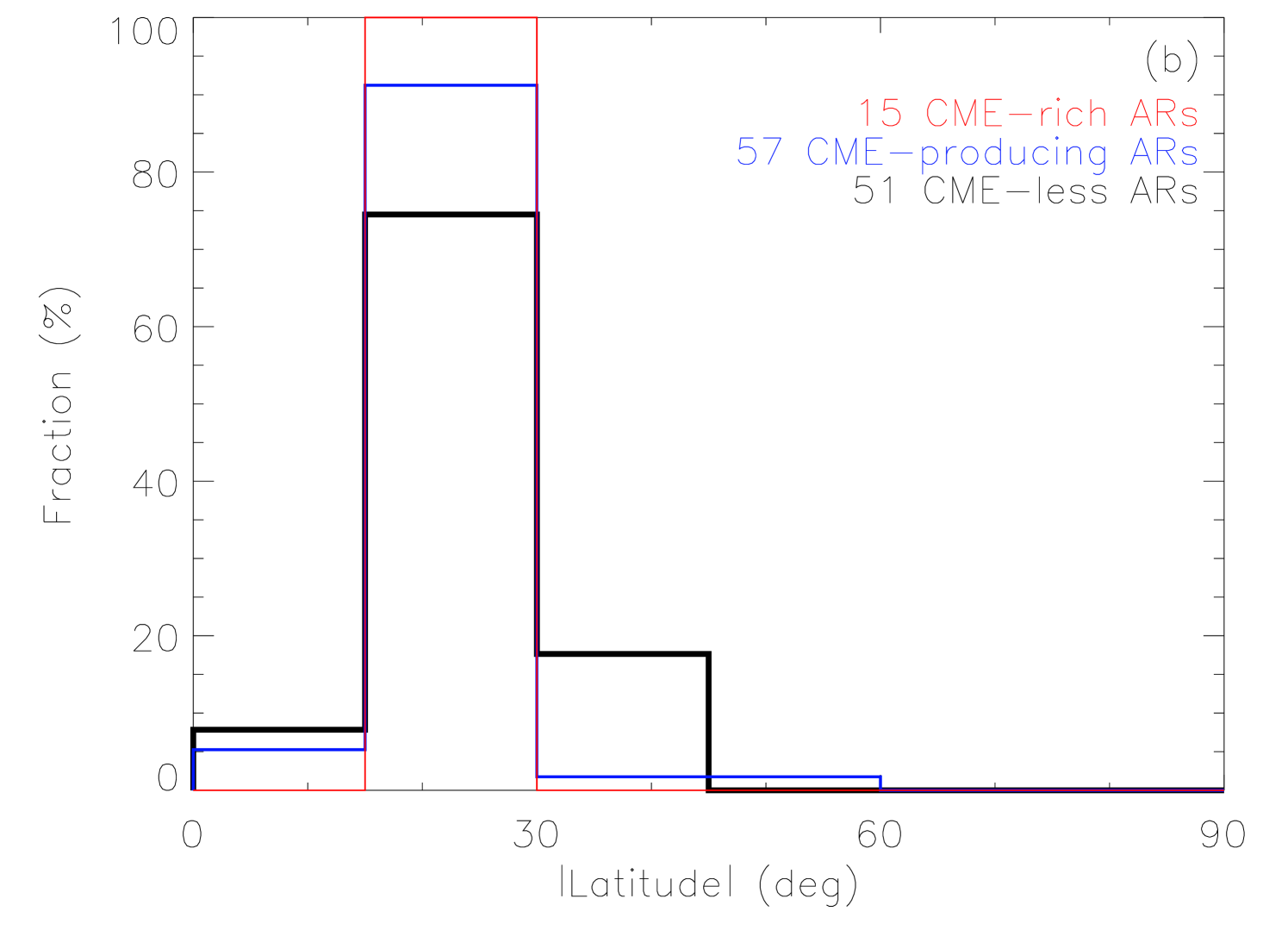
CMEs may originate from either ARs or quiet Sun regions. Reversely, ARs may frequently produce CMEs or may not produce even a single one. Why do different ARs have different CME productivity? This issue is investigated by comparing CME-less, CME-producing and CME-rich ARs. Figure 7 shows the distribution of the heliographic location (measured from the geometric center) of the 108 MDI ARs studied. The CME-less, CME-producing and CME-rich ARs are indicated in different symbols or colors (see the figure caption). All MDI ARs appeared within latitude of , and 83% of them are located in two belts between latitude of . Although the overall distributions of the different types of ARs are quite similar, there is still certain weak difference between them, which can be seen in Figure 7(b). For the CME-less ARs, there are about 25% of them occurring outside of the two AR belts. In contrast, all the CME-rich ARs locate in the two belts. Consequently, only 18% of ARs outside the two belts can produce CMEs.
Similar to what we did before, we focus on the four AR parameters: , , and . Figure 8 presents the distributions of the four AR parameters for the three different types of ARs. The CME-less, CME-producing and CME-rich ARs are plotted in black, blue and red color, respectively. It is clear that the distributions are different. A CME-producing AR tends to be larger, stronger, and more complex than a CME-less AR. Generally, all the average values of the four AR parameters for CME-producing ARs are almost twice as large as those for CME-less ARs. Further, CME-rich ARs have even larger values of the four parameters than the other two types of ARs. The average values of , , and for CME-rich ARs are about Mm2, Wb, Mm and , respectively, which are 1.7, 1.7, 1.8 and 1.8 times those of CME-producing ARs, and 2.4, 2.7, 3.6 and 2.9 times those of CME-less ARs. The fraction of the number of CME-rich ARs of all ARs in each bin is denoted by the red diamonds in Figure 8. It can be found that the fraction of CME-rich ARs generally increases with the increasing values of AR parameters. These results suggest that an AR with a larger area, stronger magnetic field and more complex morphology is more likely to be a CME-rich AR.
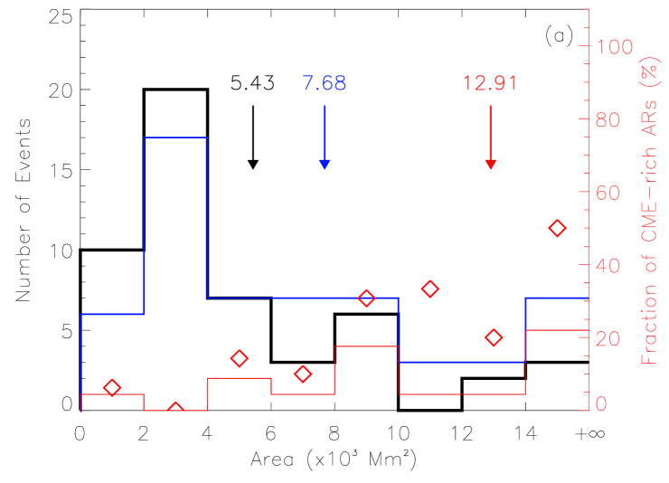
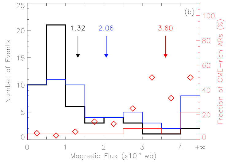
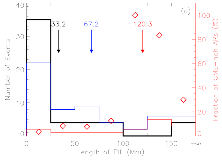
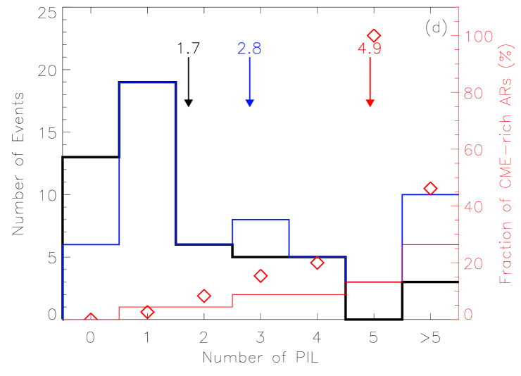
In particular, we notice that there is only one CME-rich AR with Mm2, three CME-rich ARs with Wb, two CME-rich ARs with Mm, one CME-rich AR with , and further only one CME-rich AR with all the above conditions satisfied. Thus, these values, Mm2, Wb, Mm, and , can be treated as effective thresholds, below which an AR is hard to frequently produce CMEs. Moreover, one PIL implies that the AR has a dipole field, which is the most simple topology of ARs on the Sun. Such ARs are not favorable for producing multiple CMEs. In Figure 5 of our previous paper [Wang and Zhang, 2008], we showed the distributions of the four parameters for all the 1143 MDI ARs during Carrington rotation 1911 – 2051. By comparing these thresholds to the distributions, we find that the value of each threshold is near the middle of its corresponding distribution, which means that at each side of the thresholds there are many ARs. Thus the values of these thresholds are meaningful in distinguishing CME-rich ARs from others.
Further, we use a method called linear discriminant analysis (LDA) to characterize two different classes of ARs, which have different CME productivity, in terms of these four parameters. LDA is a widely used classification method in many areas. Generally, LDA can be treated as a kind of special regression analysis. One can refer to the paper by Fisher [1936] for its principle, and refer to Sec.2.3 of our previous paper about solar prominence recognition [Wang et al., 2010] for more details of its application. In this case, we have got four parameters for all the 108 MDI ARs, and we also have known the CME productivity of these ARs. Thus we can treat these ARs as a true table, and apply the LDA to derive the optimized combination of the four parameters for discriminating between any desired two classes of ARs with different CME productivity. The optimized combination of the parameters is called linear discriminant function (LDF) and has the following form
| (2) |
where indicates the average value of the quantity for all the 108 ARs used in our LDA, and are the coefficients. The vector (, , , ) defines a hyperplane in the four dimension space of the parameters (, , , ), which best separates the two classes of ARs. In a simplified form, the optimum vector is achieved by the vector going from the mean values of the first class to the mean value of the second one, while the practical computations also involves the covariance of the distributions [Fisher, 1936].
| G | |||||
|---|---|---|---|---|---|
| CME-less vs. -producing | -0.15 | 0.20 | -0.26 | -0.07 | 0.24 |
| CME-poor vs. -rich | -0.99 | 0.87 | -0.26 | 0.64 | 0.76 |
∗ Column are the coefficients in Eq.2. The last column gives the goodness of LDF (see main text for details). The second and third row is for the discrimination between CME-less and CME-producing and between CME-poor and CME-rich, respectively.
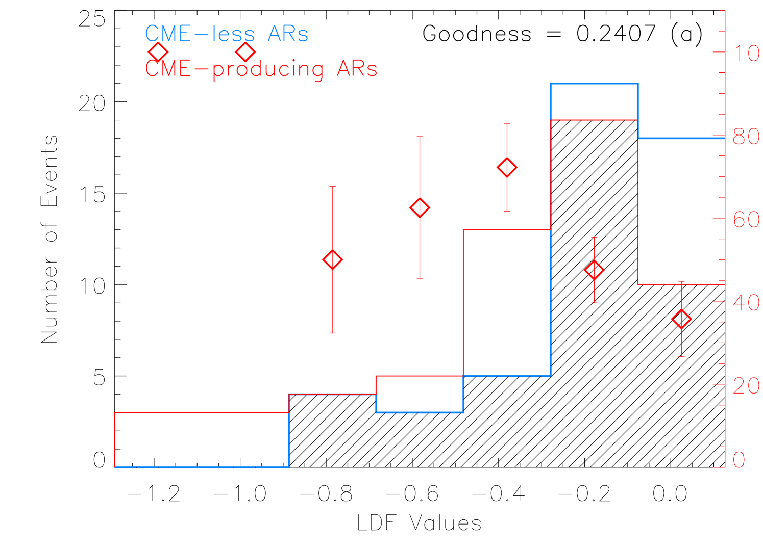
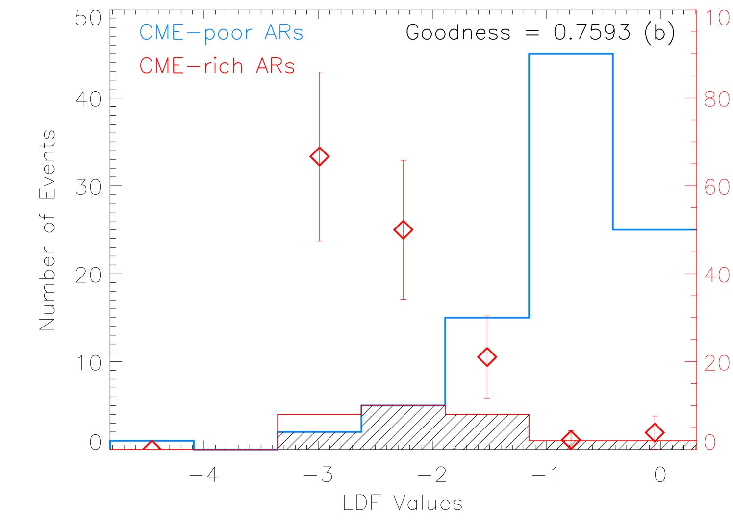
According to the LDF, one can get a one-dimensional distribution of the function value for the two different classes of ARs (as seen in Fig.9). As long as the distributions of the two different classes of ARs occupy different ranges of the value, the two classes of ARs can be more or less discriminated. Here we try to derive two LDFs for discrimination between CME-less and CME-producing ARs, and between CME-poor (CME number less than 3) and CME-rich ARs, respectively. The derived optimized coefficients have been listed in Table 3.
Figure 9 presents the LDA results. For discrimination between CME-less and CME-producing ARs (Fig.9a), the overall goodness is 0.24. It is calculated by the formula
| (3) |
where is the number of ARs whose LDF value falls within the overlap (indicated as the shadowed region in Fig.9a) and is the total number of the ARs. means the LDF being able to completely discriminate between the two different classes of ARs. The fractions of CME-producing ARs marked by the red diamonds in Figure 9(a) suggest that about 69% of ARs with LDF value are CME-producing compared with the 43% of ARs with LDF value , and particularly, all of ARs with LDF value are CME-producing. The goodness of the discrimination for CME-poor and CME-rich ARs is much better, which is 0.76 (Fig.9(b)). On the left-hand side of the LDF value of , the fraction of CME-rich ARs is about 53%, while on its right-hand side, the fraction is only about 7%. Particularly, almost all the ARs with LDF value cannot be a CME-rich AR.
5 CME-rich ARs
5.1 Pace of CME Occurrence
In certain aspects, CME-rich ARs are more interesting, especially for the purpose of space weather prediction. In our sample, there are a total of 15 CME-rich MDI ARs, which produced at least 80 CMEs. During solar minima, on average one CME occurs every other day [e.g., Gopalswamy, 2006]. Thus, a question that naturally rises is how frequently CMEs take place in these CME-rich ARs. Here we call the CMEs from the same AR same-AR CMEs. Figure 10 shows the distribution of the time interval ( so called waiting time) between two successive same-AR CMEs for these 80 CMEs. The time of the first appearance of CMEs in LASCO field of view is used to calculate the interval. It is found that the distribution can be roughly divided into two parts. The first part contains waiting times less than 15 hours and the second part longer than 15 hours. For the second part, we simply think that there is no tightly physical connection between two successive same-AR CMEs, because of the longer time interval. More attention will be put on the events of the first part. This part includes 30 data points, and manifests a unimodal distribution with a peak around hours. It can be read from the figure that about 43% of the waiting times fall into the interval of hours, and about 83% of them are between and hours. It is suggested that these successive same-AR CMEs usually occur in a pace of about hours. We would like to call these CMEs related same-AR CMEs. Few of such CMEs can take place within 2 hours or after 12 hours of a preceding CME. A further discussion of the waiting time of the related same-AR CMEs will be pursued in Sec.7.


Further, Figure 11 shows the CME productivity of these CME-rich ARs. It is found that there are actually three ARs producing 9 or more CMEs, and all the rest had produced 3 or 4 CMEs. The most productive AR had 19 CMEs (labeled as AR-a hereafter), which is NOAA AR 8210 appearing during Carrington rotation 1935. The other two most productive ARs had 11 and 9 CMEs (labeled as AR-b and AR-c), respectively. AR-b is NOAA AR 8100 appearing during Carrington rotation 1929 , while AR-c is a complex of NOAA AR 9395, 8398 and 8399 appearing during Carrington rotation 1943. Table 4 lists the three most productive ARs and related CMEs.
| For ARs | CR | Location | NOAA | ||||
|---|---|---|---|---|---|---|---|
| deg | Mm2 | Wb | Mm | AR | |||
| For CMEs | Date Time | Location | CPA | Width | Speed | ||
| UT | deg | deg | km s-1 | ||||
| AR-a | 1935 | (138, -17) | 9.68 | 3.21 | 140 | 3 | 8210 (Middle) |
| a1 | 1998/04/25 15:11 | S21E76 | 95 | 73 | 349 | ||
| a2 | 1998/04/25 18:38 | S13E73 | 70 | 17 | 324 | ||
| a3 | 1998/04/27 08:56 | S16E51 | halo | 360 | 1385 | ||
| a4 | 1998/04/29 05:31 | S16E30 | 148 | 85 | 327 | ||
| a5 | 1998/04/29 16:58 | S15E19 | halo | 360 | 1374 | ||
| a6 | 1998/05/01 23:40 | S19W02 | halo | 360 | 585 | ||
| a7 | 1998/05/02 05:31 | S17W10 | halo | 360 | 542 | ||
| a8 | 1998/05/02 14:06 | S14W15 | halo | 360 | 938 | ||
| a9 | 1998/05/02 21:20 | S20W18 | 226 | 49 | 338 | ||
| a10 | 1998/05/03 10:29 | S14W31 | 241 | 74 | 497 | ||
| a11 | 1998/05/03 22:02 | S15W35 | 317 | 194 | 649 | ||
| a12 | 1998/05/04 00:58 | S14W41 | 270 | 66 | 279 | ||
| a13 | 1998/05/04 23:27 | S20W43 | 240 | 39 | 338 | ||
| a14 | 1998/05/05 00:58 | S13W48 | 319 | 60 | 218 | ||
| a15 | 1998/05/06 00:02 | S21W59 | 274 | 110 | 786 | ||
| a16 | 1998/05/06 08:29 | S15W67 | 309 | 190 | 1099 | ||
| a17 | 1998/05/06 09:32 | S13W75 | 264 | 95 | 792 | ||
| a18 | 1998/05/07 11:05 | S15W80 | 270 | 16 | 483 | ||
| a19 | 1998/05/08 14:32 | S16W89 | 259 | 80 | 777 | ||
| AR-b | 1929 | (351, -20) | 8.31 | 2.64 | 147 | 7 | 8100 (Emerging) |
| b1 | 1997/10/29 18:21 | S19E45 | 88 | 62 | 133 | ||
| b2 | 1997/11/03 05:28 | S16W20 | 240 | 109 | 227 | ||
| b3 | 1997/11/03 09:53 | S14W18 | 238 | 71 | 338 | ||
| b4 | 1997/11/03 11:11 | S13W23 | 233 | 122 | 352 | ||
| b5 | 1997/11/04 06:10 | S15W32 | halo | 360 | 785 | ||
| b6 | 1997/11/04 15:50 | S18W32 | 242 | 5 | 266 | ||
| b7 | 1997/11/05 04:20 | S15W46 | 264 | 49 | 271 | ||
| b8 | 1997/11/05 07:29 | S16W49 | 287 | 40 | 350 | ||
| b9 | 1997/11/05 12:10 | S15W50 | 270 | 52 | 356 | ||
| b10 | 1997/11/06 12:10 | S17W62 | halo | 360 | 1556 | ||
| b11 | 1997/11/08 08:59 | S17W88 | 271 | 76 | 453 | ||
| AR-c | 1943 | (182, 20) | 35.61 | 9.14 | 122 | 5 | 8395, 8398, 8399 |
| (Decaying) | |||||||
| c1 | 1998/11/24 13:23 | N26E84 | 54 | 50 | 248 | ||
| c2 | 1998/11/24 23:30 | N32E78 | 50 | 61 | 432 | ||
| c3 | 1998/11/25 06:30 | N18E72 | 53 | 41 | 256 | ||
| c4 | 1998/11/25 14:30 | N20E73 | 57 | 52 | 213 | ||
| c5 | 1998/11/26 11:30 | N19E57 | 45 | 50 | 216 | ||
| c6 | 1998/11/28 06:30 | N20E46 | 62 | 88 | 495 | ||
| c7 | 1998/12/05 19:32 | N33W40 | 340 | 23 | — | ||
| c8 | 1998/12/06 03:54 | N34W46 | 331 | 36 | 159 | ||
| c9 | 1998/12/07 15:30 | N28W62 | 327 | 42 | 490 | ||
∗ The table lists the information of each most productive AR (bold fonts) with the corresponding CMEs (normal fonts) in the following rows. The first column numbers the ARs and CMEs. For ARs, the other columns from the left to right are Carrington Rotation (CR), Location in Carrington coordinates, area (), magnetic flux (), length and number of PILs ( and ), and the corresponding NOAA AR with its phase indicated in parentheses. For CMEs, the other columns give the date, time, location in heliographic coordinates, central position angle (), apparent width and speed.
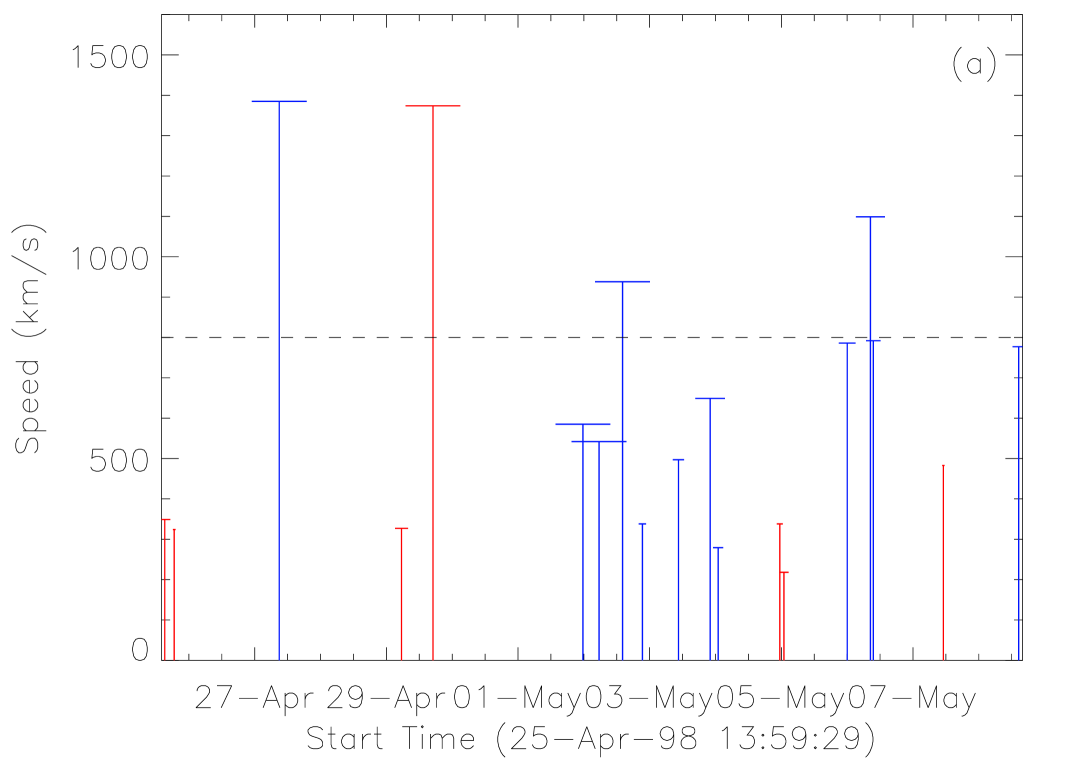
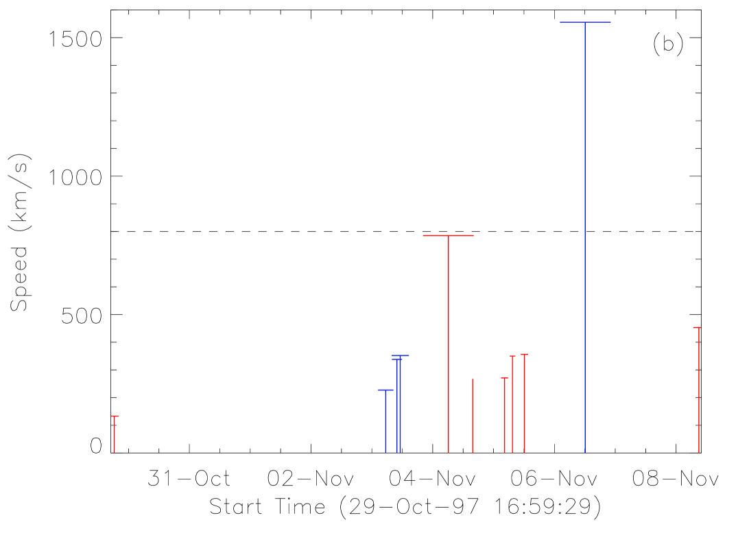
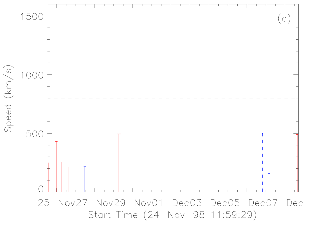
The frequency of CME occurrence of these ARs is illustrated in Figure 12. Each vertical line in the plots stands for a CME. Its length indicates the CME apparent speed and the horizontal bar at the top indicates the width. The lines with the same color mean that these CMEs are related, i.e., the time interval between two successive CMEs is shorter than 15 hours. For AR-a there are 8 groups (indicated by alternating colors of red and blue) of related same-AR CMEs, and for AR-b and AR-c there are 5 groups each. A first impression obtained from these plots is that there is only one CME that can be faster than 800 km/s in any one group, and 2 out of 3 extremely fast CMEs ( km s-1) were isolated (the other one was only grouped with another slow CME). The other 12 CME-rich ARs all follow the above regulation (not shown in the figure). Since CME speed can be used as a proxy of CME energy, or the free energy released from ARs, we simply treat a CME faster than 800 km s-1 as a strong CME, and others as weak CMEs. The above facts imply that (1) the total free magnetic energy stored in an AR at any instant can usually support at most one strong CME and several weak CMEs, and (2) an AR has to take more than 15 hours to re-accumulate sufficient free energy to produce another strong CME.
| No | CR | Location | NOAA | ||||
|---|---|---|---|---|---|---|---|
| deg | Mm2 | Wb | Mm | AR | |||
| 1 | 1920 | (205, 7) | 8.17 | 1.67 | 0 | 0 | 8020 () |
| 2 | 1922 | ( 14, 5) | 4.21 | 1.43 | 62 | 2 | 8040 () |
| 3 | 1923 | (188, -28) | 3.86 | 1.01 | 17 | 1 | 8048 () |
| 4 | 1926 | (268, 26) | 6.17 | 1.18 | 0 | 0 | 8074 () |
| 5 | 1926 | (279, 16) | 2.48 | 0.54 | 0 | 0 | 8073 () |
| 6 | 1926 | ( 11, 34) | 3.10 | 0.61 | 6 | 1 | 8081 () |
| 7 | 1927 | (225, 28) | 8.19 | 2.01 | 15 | 1 | 8086 () |
| 8 | 1927 | ( 97, -24) | 6.84 | 1.19 | 8 | 1 | 8087 () |
| 9 | 1927 | (363, 22) | 4.48 | 1.08 | 18 | 2 | 8082 () |
| 10 | 1928 | (342, -30) | 2.79 | 0.52 | 18 | 1 | 8090 () |
| 11 | 1928 | ( 22, 18) | 2.91 | 0.61 | 25 | 3 | 8099 () |
| 12 | 1929 | (303, 23) | 4.88 | 1.08 | 60 | 3 | 8103 () |
| 13 | 1929 | ( 91, -19) | 2.67 | 0.60 | 11 | 1 | 8109 () |
| 14 | 1930 | (352, -20) | 14.01 | 2.68 | 0 | 0 | 8112 () |
| 15 | 1930 | (358, 25) | 2.79 | 0.52 | 0 | 0 | 8111 () |
| 16 | 1930 | (287, -29) | 1.26 | 0.25 | 0 | 0 | 8114 () |
| 17 | 1931 | (345, -23) | 13.68 | 3.75 | 156 | 2 | 8124 () |
| 18 | 1932 | (278, -37) | 6.66 | 1.82 | 72 | 4 | 8143 () |
| 19 | 1932 | ( 14, -20) | 3.31 | 0.63 | 10 | 1 | 8158 () |
| 20 | 1932 | (267, 14) | 3.55 | 0.89 | 0 | 0 | 8144 () |
| 21 | 1932 | ( 24, 26) | 2.47 | 0.57 | 0 | 0 | 8157 () |
| 22 | 1933 | ( 62, -40) | 8.16 | 2.26 | 69 | 4 | 8176 () |
| 23 | 1933 | (360, 22) | 3.97 | 0.72 | 16 | 1 | 8160 () |
| 24 | 1934 | (240, -24) | 18.22 | 4.93 | 161 | 6 | 8185, 8189 () |
| 25 | 1934 | ( 83, -23) | 8.25 | 2.76 | 48 | 3 | 8193, 8199 () |
| 26 | 1935 | (386, -23) | 40.52 | 10.17 | 151 | 10 | 8195, 8194, 8198, 8200, |
| 8202 () | |||||||
| 27 | 1935 | (356, 18) | 2.65 | 0.48 | 11 | 1 | 8201 () |
| 28 | 1936 | (282, 22) | 12.97 | 3.31 | 92 | 4 | 8222 () |
| 29 | 1936 | (282, -27) | 8.65 | 2.27 | 85 | 4 | 8220 () |
| 30 | 1937 | (283, 22) | 5.30 | 0.92 | 0 | 0 | 8238, 8239 () |
∗ The column arrangement is as the same as that for ARs in Table 4 except that the parentheses in the last column give the most complicated type of the AR associated sunspot group during the AR crossing the visible disk.
Kienreich et al. [2011] reported four homologous CME-associated coronal waves observed by STEREO. It is found that the waiting times between the eruptions have a positive correlation with the strength of the eruptions. This case study suggests that from the same AR a stronger eruption needs a longer waiting time, which is consistent with our statistical results.
5.2 Most Productive ARs vs. CME-less ARs
MDI daily magnetogram images indicate that all the three CME-productive ARs discussed above rotated from the solar east limb to west limb, and lasted at least for about 13 days. AR-a, i.e., NOAA AR 8210, has been studied by several researchers. Subramanian and Dere [2001] pointed out that the life time of this AR is about days, and it was in the mid-phase when it appeared in the front-side of the Sun during Carrington rotation 1935. The type of the sunspots associated with this AR changed among , , and , indicating its complexity in morphology. AR-b is also a complex AR. Different from AR-a, it was obviously emerging on its way crossing the field of view. Its associated sunspots developed from type of to and around 1997 November 2 – 4, during and after which all the CMEs except one launched. AR-c was more complicated than AR-a and AR-b, which consisted of three NOAA ARs. Our AR-detection method merges the three NOAA ARs together as a single compound region, as it is indeed difficult to separate them as viewed in magnetograms (an AR appears much bigger in the magnetogram images than in the white light image). AR-c was probably in the decaying phase. From MDI magnetograms, one may notice that this AR was much more diffusive than other two. The average magnetic field of AR-a and AR-b was larger than 300 G, whereas that of AR-c was about 250 G. There were several sunspot groups in the AR, but their types are or , relatively simpler than those in other two ARs. Thus, AR-c was a globally complex, but locally simple and weak AR. This is probably why AR-c produced 9 CMEs but none of these CMEs was faster than 500 km s-1.
As a comparison, we look into CME-less ARs. It is found that 19 out of 51 () CME-less ARs have more than one PILs, and only 4 () CME-less ARs have the PILs’ total length longer than 100 Mm. Further, we checked the MDI magnetograms and NOAA AR list, and selected the CME-less ARs that have corresponding NOAA ARs and showed in rotation from the solar east limb to west limb. There are a total of 30 such CME-less ARs. Table 5 lists these ARs for reference. The sunspot classification suggests that about 90% of these ARs are very simple, belonging to or type, and the other 10% are . Note that the sunspot type we provide here is the most complex type during its passage. We also investigated the MDI movies, and found that most of these ARs are in the mid-phase of its whole life, and some in emerging phase and others in decaying phase. Compared with the most productive ARs, the above results suggest that the CME productivity of ARs is strongly related with the AR complexity, but less related with the AR phase.
6 Conclusions
In this paper, 224 location-identified CMEs and the corresponding 108 MDI ARs during 1997 – 1998 are investigated. The association between CMEs and ARs suggests that about of the CMEs are related with ARs, and at least about of the ARs produce one or more CME during one disk passage. Some ARs frequently produce CMEs; there are 15 CME-rich ARs, which produced a total of at least 80 CMEs, and the most productive AR produced 19 CMEs. By analyzing the relationship between the properties of CMEs and ARs, the following conclusions are reached. These conclusions mostly confirm the previous studies [e.g., Guo et al., 2007; Falconer et al., 2008; Yeates et al., 2010] but with significant additions.
-
1.
There is no evident difference between AR-related and non-AR-related CMEs in terms of CME speed, acceleration and width, which suggests that the concept of two types of CMEs [e.g., Sheeley, Jr. et al., 1999] may not be true, or at least they can not be simply attributed to their source regions.
-
2.
There is no evident dependence of CME speed on the AR area, magnetic flux and complexity, though a trend that an AR with larger area, stronger magnetic field and more complex morphology has a higher possibility of producing extremely fast CMEs (speed km s-1) was found before [Wang and Zhang, 2008]. However, the CME width manifests a weak correlation with the AR parameters, and the area and magnetic flux are two important factors.
-
3.
CME-producing ARs more likely appear in the two latitudinal belts at than CME-less ARs. Particularly, all CME-rich ARs are located in the belts, and only 18% of the ARs outside the two belts can produce CMEs.
-
4.
CME-producing ARs tend to be larger, stronger and more complex than CME-less ARs. All the average values of , , and of CME-producing ARs are almost twice as large as those of CME-less ARs. For CME-rich ARs, the average values are even larger, which are 2.4, 2.7, 3.6 and 2.9 times those of CME-less ARs.
-
5.
There seem to be thresholds of Mm2, Wb and Mm, below which an AR is hard to frequently produce CMEs. Particularly, a dipolar-field AR is not favorable for producing multiple CMEs. The discriminant analysis shows that almost all the ARs with the LDF value larger than cannot be a CME-rich AR.
-
6.
The sunspots in all the three most productive ARs (creating 9 or more CMEs) at least belong to type, whereas 90% of those in the CME-less ARs are or type, and only 10% type. It is suggested that the CME productivity of ARs is strongly related with the AR complexity, but less related with its phase.
-
7.
Combining the above results, we can claim that the size, strength and complexity of ARs do little with the kinematic properties of CMEs, but have significant effects on the CME productivity.
The CME-rich ARs are then investigated particularly. Through the analysis of the waiting times of the same-AR CMEs, it is found that the distribution of the waiting times consists of two parts with a separation at about 15 hours, which implies two different patterns of the occurrences of same-AR CMEs, and those CMEs with a waiting time shorter than 15 hours are probably truly physical related. A detailed analysis of these related same-AR CMEs further gives rise to the following two interesting conclusions.
-
1.
The average waiting time of related same-AR CMEs is about 8 hours, which means that a CME-productive AR tends to produce CMEs at a pace of 8 hours.
-
2.
An AR cannot produce two or more CMEs faster than 800 km s-1 within a time interval of 15 hours (i.e., in any group of related same-AR CMEs).
It should be noted that all the above conclusions are established on the statistical study of CMEs and ARs near the minimum of solar cycle 23. Whether or not they also reflect the fact during solar maximum needs to be verified by further work.
7 Preliminary Discussion On The CME Waiting Time
A CME is a process of releasing a huge amount of free magnetic energy stored in the corona. Sufficient amount of free magnetic energy is a necessary condition for an AR to produce a CME [e.g., Priest and Forbes, 2002; Régnier and Priest, 2007]. Many previous studies also suggested that sufficient large helicity injection is critical for a solar eruption [e.g., Démoulin et al., 2002; Nindos and Zhang, 2002; Nindos et al., 2003; Green et al., 2002, 2003; LaBonte et al., 2007; Smyrli et al., 2010]. Our statistical analysis results of CME waiting times naturally raise two issues. One (labeled as I1) is why CME-rich ARs frequently produce CMEs, especially why in a pace of about 8 hours. The other (labeled as I2) is why there can be at most one strong CME (speed km s-1) in any group of related same-AR CMEs or within an interval of 15 hours? Note, the value of speed 800 km s-1 is underestimated because of the projection effect. Moreover, we believe that the values of 8 hours, 15 hours and 800 km s-1, might slightly vary if more CME-rich ARs during solar maximum are included in the statistical sample. No matter what the exact values are, to satisfactorily address the two issues, we need much more work. The unprecedented data from SDO mission, which have much higher resolution in both space and time than SOHO data, may help us deepening our understanding of the nature of same-AR CMEs. Here, we would like to carry out a preliminary discussion on the two issues. For issue I1, we think that it implies at least three possible mechanisms of the related same-AR CMEs.
(1) The related same-AR CMEs come from the same part of an AR. The AR is able to quickly refill enough free energy or helicity after it is consumed by a CME, so that multiple CMEs can be launched from the same place. In this scenario, our statistical results imply that the time-scale of the refilling is about 8 hours. LaBonte et al. [2007] surveyed 48 X-class flare-producing regions and found that these regions consistently had a larger helicity change than non-flaring regions. Particularly, they found that most of the X-flare regions can accumulate helicity for a CME in a few days to a few hours. For example, the typical time of helicity injection for NOAA AR 10486 to repeatedly produce CMEs is about 10 hours. Kienreich et al. [2011] reported four homologous CME-associated coronal waves observed by STEREO. The waiting times between them are around 2.5 hours, and it is found that the waiting time has a positive correlation with the strength of the eruption. However, more events show a much longer waiting time. Also in the paper by LaBonte et al. [2007], the waiting time for NOAA AR 10720 is about 19 hours. Li et al. [2010] study of the homologous CMEs during 1997 May 5 –16 showed that sufficient energy is built up on the order of several days. Homologous CMEs not only originate from the same source region but also have the similar morphology. They can be considered as a special type of same-AR CMEs. We suggest that such long-waiting-time CMEs in Li et al. [2010] study should belong to the second part of our distribution (Fig.10), and probably have a different cause.
(2) There are several magnetic flux systems in the AR, which are all possible to develop into a CME, and the eruption of one of them may cause others unstable and eventually erupting. In this scenario, the time-scale of the unstabilization caused by the preceding CME is typically 8 hours. The MHD numerical simulation by Peng and Hu [2007] provided such possibility in theory. In their simulation, multi-polar magnetic configuration, which contains three arcade systems, is set, and shearing motions are introduced to build up free energy. It is found that an arcade may form a flux rope and then erupt by the shearing motion of its adjacent arcades. The study of the two successive CMEs originating from NOAA AR 10808 on 2005 September 13 by Liu et al. [2009] is an observational evidence. Their analysis suggested that the launch of the second CME was contributed by the first CME which partially removed the overlying magnetic fields in the northern part of the AR.
(3) The related same-AR CMEs might come from the different parts of the same magnetic flux system in the AR. The eruption of one part may cause the other parts further erupting. This scenario is similar to but not same as the second one, and the time-scale of unstabilization is also required to be about 8 hours. An observational case supporting it is the 2005 May 13 CMEs studied by Dasso et al. [2009]. In their work, they found that the giant ICME observed by ACE on May 15 actually consisted of two magnetic clouds, which were corresponding to two CMEs originating from NOAA AR 10759 on May 13. The much more detailed multi-wavelength analysis further showed that the two CMEs were formed from the magnetic fields above the different portion of the same filament (or PIL), and the waiting time is about 4 hours. There are also some other studies showing that different portions of the same filament may erupt successively [e.g., Maltagliati et al., 2006; Gibson et al., 2006; Liu et al., 2008].
Which one is most likely to work for the related same-AR CMEs? To answer this question, we need to carefully check the erupting process of each CME with multiple-wavelength data, especially the exact locations that the CMEs originate. This will be done in a separate paper.
For issue I2, we think that the key point is the rate of free energy accumulation. According to previous statistical studies [e.g., Vourlidas et al., 2000], the mass of a CME is typically kg. Thus a speed of 800 km s-1 corresponds to a kinetic energy of J. It is also showed that the injected thermal energy during a CME is on the same order of its kinetic energy [e.g., Akmal et al., 2001; Ciaravella et al., 2001; Rakowski et al., 2007]. In our study, CME speeds were measured in the field of view of SOHO/LASCO, which is beyond . Thus the gravitational potential energy of a CME is considerable, which can be estimated as about J under the assumption of the CME mass equal to kg and moved from the heliocentric distance to beyond . The sum of thermal, kinetic and potential energies meet the minimum requirement of the free energy for an AR to produce a CME with a speed of 800 km s-1. The actual free energy released during the CME should also include radiation energy, like flares. Relating the minimum required free energy with the waiting time of at least 15 hours, we can estimate that the rate of an AR accumulating free energy is on the order of J s-1. This value is a very coarse estimation, because CME mass, speed and waiting time are all very different case by case.
Recently, Li et al. [2011] proposed a so-called ‘twin-CME’ scenario to explain ground level events (GLEs). In their model, they found that two CMEs successively erupting from the same (or nearby) AR in 8.7 hours are favorable for the generation of GLEs. The duration of 8.7 hours represents the characteristic time for a turbulence decayed away. Their scenario is apparently supported by the GLEs observations in solar cycle 23 (Table 1 in their paper). Does the number 8.7 have any underlying physical relationship with our 8 hours? It is worthy of follow-up studies.
In short, we would like to highlight the values, 8 hours, 15 hours, 800 km s-1 and J s-1 derived/estimated from our statistical study. These values can serve as constraints for AR and/or CME modeling, and further deepen our understanding of the mechanism of AR energy accumulation and release.
Acknowledgements.
We acknowledge the use of the data from SOHO/MDI and the CDAW CME catalog, which is generated and maintained at the CDAW Data Center by NASA and The Catholic University of America in cooperation with the Naval Research Laboratory. SOHO is a project of international cooperation between ESA and NASA. We thank the anonymous referees for their kindly comments and corrections. This research is supported by grants from 973 key project 2011CB811403, NSFC 41131065, 40904046, 40874075, 41121003, CAS 100-Talent Program, KZCX2-YW-QN511 and startup fund, FANEDD 200530, and the fundamental research funds for the central universities. J.Z. was supported by NSD grant ATM-0748003 and NASA grant NNG05GG19G.References
- Akiyama et al. [2007] Akiyama, S., S. Yashiro, and N. Gopalswamy, The CME-productivity associated with flares from two active regions, Adv. in Space Res., 39, 1467–1470, 2007.
- Akmal et al. [2001] Akmal, A., J. C. Raymond, A. Vourlidas, B. Thompson, A. Ciaravella, Y.-K. Ko, M. Uzzo, and R. Wu, SOHO observations of a coronal mass ejection, Astrophys. J., 553, 922–934, 2001.
- Andrews and Howard [2001] Andrews, M. D., and R. A. Howard, A two-type classification of lasco coronal mass ejection, Space Sci. Rev., 95, 147–163, 2001.
- Canfield et al. [1999] Canfield, R. C., H. S. Hudson, and D. E. McKenzie, Sigmoidal morphology and eruptive solar activity, Geophys. Res. Lett., 26, 627–630, 1999.
- Chen et al. [2006] Chen, A. Q., P. F. Chen, and C. Fang, On the CME velocity distribution, Astron. & Astrophys., 456, 1153–1158, 2006.
- Ciaravella et al. [2001] Ciaravella, A., J. C. Raymond, F. Reale, L. Strachan, and G. Peres, 1997 December 12 helical coronal mass ejection. II. density, energy estimates, and hydrodynamics, Astrophys. J., 557, 351–365, 2001.
- Dasso et al. [2009] Dasso, S., C. H. Mandrini, B. Schmieder, H. Cremades, C. Cid, Y. Cerrato, E. Saiz, P. Démoulin, A. N. Zhukov, L. Rodriguez, A. Aran, M. Menvielle, and S. Poedts, Linking two consecutive nonmerging magnetic clouds with their solar sources, J. Geophys. Res., 114, A02,109, 2009.
- Delannée et al. [2000] Delannée, C., J.-P. Delaboudinière, and P. Lamy, Observation of the origin of cmes in the low corona, Astron. & Astrophys., 355, 725–742, 2000.
- Démoulin et al. [2002] Démoulin, P., C. H. Mandrini, L. van Driel-Gesztelyi, B. J. Thompson, S. Plunkett, Z. Kővári, G. Aulanier, and A. Young, What is the source of the magnetic helicity shed by cmes? the long-term helicity budget of ar 7978, Astron. & Astrophys., 382, 650–665, 2002.
- Falconer et al. [2002] Falconer, D. A., R. L. Moore, and G. A. Gary, Correlation of the coronal mass ejection productivity of solar active regions with measures of their global nonpotentiality from vector magnetograms: Baseline results, Astrophys. J., 569, 1016–1025, 2002.
- Falconer et al. [2006] Falconer, D. A., R. L. Moore, and G. A. Gary, Magnetic causes of solar coronal mass ejections: Dominance of the free magnetic energy over the magnetic twist alone, Astrophys. J., 644, 1258–1272, 2006.
- Falconer et al. [2008] Falconer, D. A., R. L. Moore, and G. A. Gary, Magnetogram measures of total nonpotentiality for prediction of solar coronal mass ejections from active regions of any degree of magnetic complexity, Astrophys. J., 689, 1433–1442, 2008.
- Falconer et al. [2009] Falconer, D. A., R. L. Moore, G. A. Gary, and M. Adams, The “main sequence” of explosive solar active regions: Discovery and interpretation, Astrophys. J., 700, L166–L169, 2009.
- Feynman and Ruzmaikin [2004] Feynman, J., and A. Ruzmaikin, A high-speed erupting-prominence CME: A bridge between types, Sol. Phys., 219, 301–313, 2004.
- Fisher [1936] Fisher, R. A., The use of multiple measurements in taxonomic problems, Annals of Eugenics, 7, 179–188, 1936.
- Georgoulis and Rust [2007] Georgoulis, M. K., and D. M. Rust, Quantitative forecasting of major solar flares, Astrophys. J., 661, L109–L112, 2007.
- Gibson et al. [2006] Gibson, S. E., Y. Fan, T. Török, and B. Kliem, The evolving sigmoid: Evidence for magnetic flux ropes in the corona before, during, and after CMEs, Space Sci. Rev., 124, 131–144, 2006.
- Gopalswamy [2006] Gopalswamy, N., Coronal mass ejections of solar cycle 23, J. Astrophys. Astron., 27, 243–254, 2006.
- Green et al. [2002] Green, L. M., S. A. Matthews, L. van Driel-Gesztelyi, L. K. Harra, and J. L. Culhane, Multi-wavelength observations of an X-class flare without a coronal mass ejection, Sol. Phys., 205, 325–339, 2002.
- Green et al. [2003] Green, L. M., P. Démoulin, C. H. Mandrini, and L. van Driel-Gesztelyi, How are emerging flux, flares and CMEs related to magnetic polarity imbalance in MDI data, Sol. Phys., 215, 307–325, 2003.
- Guo et al. [2007] Guo, J., H. Q. Zhang, and O. V. Chumak, Magnetic properties of flare-CME productive active regions and CME speed, Astron. & Astrophys., 462, 1121–1126, 2007.
- Jing et al. [2006] Jing, J., H. Song, V. Abramenko, C. Tan, and H. Wang, The statistical relationship between the photospheric magnetic parameters and the flare productivity of active regions, Astrophys. J., 644, 1273–1277, 2006.
- Kienreich et al. [2011] Kienreich, I. W., A. M. Veronig, N. Muhr, M. Temmer, B. Vršnak, and N. Nitta, Case study of four homologous large-scale coronal waves observed on 2010 april 28 and 29, Astrophys. J. Lett., 727, L43(6pp), 2011.
- LaBonte et al. [2007] LaBonte, B. J., M. K. Georgoulis, and D. M. Rust, Survey of magnetic helicity injection in regions producing X-class flares, Astrophys. J., 671, 955–963, 2007.
- Leka and Barnes [2003] Leka, K. D., and G. Barnes, Photospheric magnetic field properties of flaring versus flare-quiet active regions. ii. discriminant analysis, Astrophys. J., 595, 1296–1306, 2003.
- Leka and Barnes [2007] Leka, K. D., and G. Barnes, Photospheric magnetic field properties of flaring versus flare-quiet active regions. iv. a statistically significant sample, Astrophys. J., 656, 1173–1186, 2007.
- Li et al. [2011] Li, G., R. Moore, R. A. Mewaldt, L. Zhao, and A. Labrador, A twin-CME scenario for ground level events, Space Sci. Rev., p. submitted, 2011.
- Li et al. [2010] Li, Y., B. J. Lynch, B. T. Welsch, G. A. Stenborg, J. G. Luhmann, G. H. Fisher, Y. Liu, and R. W. Nightingale, Sequential coronal mass ejections from AR8038 in May 1997, Sol. Phys., 264, 149–164, 2010.
- Liu et al. [2009] Liu, C., J. Lee, M. Karlicky, D. P. Choudhary, N. Deng, and H. Wang, Successive solar flares and coronal mass ejections on 2005 september 13 from NOAA AR 10808, Astrophys. J., 703, 757–768, 2009.
- Liu et al. [2008] Liu, R., H. R. Gilbert, D. Alexander, and Y. Su, The effect of magnetic reconnection and writhing in a partial filament eruption, Astrophys. J., 680, 1508–1515, 2008.
- MacQueen and Fisher [1983] MacQueen, R. M., and R. R. Fisher, The kinematics of solar inner coronal transients, Sol. Phys., 89, 89–102, 1983.
- Maeshiro et al. [2005] Maeshiro, T., K. Kusano, T. Yokoyama, and T. Sakurai, A statistical study of the correlation between magnetic helicity injection and soft x-ray activity in solar active regions, Astrophys. J., 620, 1069–1084, 2005.
- Maltagliati et al. [2006] Maltagliati, L., A. Falchi, and L. Teriaca, Rhessi images and spectra of two small flares, Sol. Phys., 235, 125–146, 2006.
- Moon et al. [2002] Moon, Y.-J., G. S. Choe, H. Wang, Y. D. Park, N. Gopalswamy, G. Yang, and S. Yashiro, A statistical study of two classes of coronal mass ejections, Astrophys. J., 581, 694–702, 2002.
- Nindos and Zhang [2002] Nindos, A., and H. Zhang, Photospheric motions and coronal mass ejection productivity, Astrophys. J., 573, L133, 2002.
- Nindos et al. [2003] Nindos, A., J. Zhang, and H. Zhang, The magnetic helicity budget of solar active regions and coronal mass ejections, Astrophys. J., 594, 1033–1048, 2003.
- Peng and Hu [2007] Peng, Z., and Y.-Q. Hu, Interaction between adjacent sheared magnetic arcades in the solar corona, Astrophys. J., 668, 513–519, 2007.
- Priest and Forbes [2002] Priest, E. R., and T. G. Forbes, The magnetic nature of solar flares, Astron. & Astrophys. Rev., 10, 313–377, 2002.
- Rakowski et al. [2007] Rakowski, C. E., J. M. Laming, and S. T. Lepri, Ion charge states in halo coronal mass ejections: What can we learn about the explosion?, Astrophys. J., 667, 602–609, 2007.
- Régnier and Priest [2007] Régnier, S., and E. R. Priest, Free magnetic energy in solar active regions above the minimum-energy relaxed state, Astrophys. J., 669, L53–L56, 2007.
- Sammis et al. [2000] Sammis, I., F. Tang, and harold Zirin, The dependence of large flare occurrence on the magnetic structure of sunspots, Astrophys. J., 540, 583–587, 2000.
- Schrijver [2007] Schrijver, C. J., A characteristic magnetic field pattern associated with all major solar flares and its use in flare forecasting, Astrophys. J., 655, L117–L120, 2007.
- Schrijver [2009] Schrijver, C. J., Driving major solar flares and eruptions, Adv. in Space Res., 43, 739–755, 2009.
- Sheeley, Jr. et al. [1999] Sheeley, Jr., N. R., J. H. Walters, Y.-M. Wang, and R. A. Howard, Continuous tracking of coronal outflows: Two kinds of coronal mass ejections, J. Geophys. Res., 104, 24,739–24,768, 1999.
- Smyrli et al. [2010] Smyrli, A., F. Zuccarello, P. Romano, F. P. Zuccarello, S. L. Guglielmino, D. Spadaro, A. W. Hood, and D. Mackay, Trend of photospheric magnetic helicity flux in active regions generating halo coronal mass ejections, Astron. & Astrophys., 521, A56, 2010.
- St. Cyr et al. [1999] St. Cyr, O. C., J. T. Burkepile, A. J. Hundhausen, and A. R. Lecinski, A comparison of ground-based and spacecraft observations of coronal mass ejections from 1980–1989, J. Geophys. Res., 104, 12,493–12,506, 1999.
- Su et al. [2007] Su, Y., A. Van Ballegooijen, J. McCaughey, E. Deluca, K. K. Reeves, and L. Golub, What determines the intensity of solar flare/CME events?, Astrophys. J., 665, 1448–1459, 2007.
- Subramanian and Dere [2001] Subramanian, P., and K. P. Dere, Source regions of coronal mass ejections, Astrophys. J., 561, 372, 2001.
- Svestka and Cliver [1992] Svestka, Z., and E. W. Cliver, History and basic characteristics of eruptive flares, in Eruptive Solar Flares, edited by Z. Svestka, B. V. Jackson, and M. E. Machado, Proceedings of IAU Colloquium No. 113, pp. 1–11, Springer-Verlag, New York, 1992.
- Ternullo et al. [2006] Ternullo, M., L. Contarino, P. Romano, and F. Zuccarello, A statistical analysis of sunspot groups hosting m and x flares, Astron. Nachr., 327, 36–43, 2006.
- Vourlidas et al. [2000] Vourlidas, A., P. Subramanian, K. P. Dere, and R. A. Howard, Large-angle spectrometric coronagraph measurements of the energetics of coronal mass ejections, Astrophys. J., 534, 456–467, 2000.
- Vršnak et al. [2005] Vršnak, B., D. Sudar, and D. Ruždjak, The CME-flare relationship: Are there really two types of CMEs?, Astron. & Astrophys., 435, 1149–1157, 2005.
- Wang and Zhang [2007] Wang, Y., and J. Zhang, A comparative study between eruptive x-class flares associated with coronal mass ejections and confined x-class flares, Astrophys. J., 665, 1428, 2007.
- Wang and Zhang [2008] Wang, Y., and J. Zhang, A statistical study on solar active regions producing extremely fast coronal mass ejections, Astrophys. J., 680, 1516, 2008.
- Wang et al. [2010] Wang, Y., H. Cao, J. Chen, T. Zhang, S. Yu, H. Zheng, C. Shen, J. Zhang, and S. Wang, Solar limb prominence catcher and tracker (SLIPCAT): An automated system and its preliminary statistical results, Astrophys. J., 717, 973–986, 2010.
- Wang et al. [2011] Wang, Y., C. Chen, B. Gui, C. Shen, P. Ye, and S. Wang, Statistical study of coronal mass ejection source locations: Understanding cmes viewed in coronagraphs, J. Geophys. Res., 116, A04,104, doi:10.1029/2010JA016,101, 2011.
- Yeates et al. [2010] Yeates, A. R., G. D. R. Attrill, D. Nandy, D. H. Mackay, P. C. H. Martens, and A. A. van Ballegooijen, Comparison of a global magnetic evolution model with observations of coronal mass ejections, Astrophys. J., 709, 1238–1248, 2010.
- Yurchyshyn et al. [2005] Yurchyshyn, V., S. Yashiro, V. Abramenko, H. Wang, and N. Gopalswamy, Statistical distributions of speeds of coronal mass ejections, Astrophys. J., 619, 599–603, 2005.
- Zhang et al. [2010] Zhang, J., Y. Wang, and Y. Liu, Statistical properties of solar active regions obtained from an automatic detection system and the computational biases, Astrophys. J., 723, 1006–1018, 2010.
- Zhou et al. [2003] Zhou, G., J. Wang, and Z. Cao, Correlation between halo coronal mass ejections and solar surface activity, Astron. & Astrophys., 397, 1057, 2003.