Statistical Taylor Expansion¹¹1

Chengpu Wang
40 Grossman Street, Melville, NY 11747, USA
Chengpu@gmail.com

(2024/09/30)

Abstract

Statistical Taylor expansion replaces the input precise variables in a conventional Taylor expansion with random variables each with known distribution, to calculate the result mean and deviation. It is based on the uncorrelated uncertainty assumption [1]: Each input variable is measured independently with fine enough statistical precision, so that their uncertainties are independent of each other. Statistical Taylor expansion reveals that the intermediate analytic expressions can no longer be regarded as independent of each other, and the result of analytic expression should be path independent. This conclusion differs fundamentally from the conventional common approach in applied mathematics to find the best execution path for a result. This paper also presents an implementation of statistical Taylor expansion called variance arithmetic, and the tests on variance arithmetic.

Keywords: computer arithmetic, error analysis, interval arithmetic, uncertainty, numerical algorithms.

AMS subject classifications: G.1.0

1 Introduction

1.1 Measurement Uncertainty

Except for the simplest counting, scientific and engineering measurements never give completely precise results [2][3]. In scientific and engineering measurements, the uncertainty of a measurement $x$ usually is characterized by either the sample deviation $\delta x$ or the uncertainty range $\Delta x$ [2][3].

•

If $\delta x=0$ or $\Delta x=0$ , $x$ is a precise value.
•

Otherwise, $x$ is an imprecise value.

$P(x)\equiv\delta x/|x|$ is defined as the statistical precision (or simply precision in this paper) of the measurement, in which $x$ is the value, and $\delta x$ is the uncertainty deviation. A larger precision means a coarser measurement while a smaller precision means finer measurement. The precision of measured values ranges from an order-of-magnitude estimation of astronomical measurements to $10^{-2}$ to $10^{-4}$ of common measurements to $10^{-14}$ of state-of-art measurements of basic physics constants [4].

How to calculate the analytic expression with imprecise values is the subject of this paper.

1.2 Extension to Existing Statistics

Instead of focusing on the result uncertainty distribution of a function [5], statistical Taylor expansion gives the result mean and variance for general analytic expressions.

•

The effect of input uncertainty to output value has only been given for special case [6]. Statistical Taylor expansion generalizes it as uncertainty bias in Formula (2.6), and (2.9) in this paper.
•

The traditional variance-covariance framework only considers linear interaction between random variables through an analytic function [5][6]. Statistical Taylor expansion generalizes it to higher order as Formula (2.3) in this paper.

1.3 Problem of the Related Numerical Arithmetics

Variance arithmetic implements statistical Taylor expansion. It exceeds all existing related numerical arithmetics.

1.3.1 Conventional Floating-Point Arithmetic

The conventional floating-point arithmetic [7][8][9] assumes the finest precision for each value all the time, and constantly generates artificial information to meet this assumption during the calculation [10]. For example, the following calculation is carried out precisely in integer format:

64919121\times 205117922-159018721\times 83739041=\\ 13316075197586562-13316075197586561=1;

(1.1)

If Formula (1.1) is carried out using conventional floating-point arithmetic:

64919121\times 205117922-159018721\times 83739041=\\ 64919121.000000000\times 205117922.000000000-159018721.000000000\times 83739041.000000000=\\ 13316075197586562.-13316075197586560.=2.=2.0000000000000000;

(1.2)

1.

The normalization of the input values pads zero tail bit values artificially, to make each value as precise as possible for the 64-bit IEEE floating-point representation, e.g., from $64919121$ to $64919121.000000000$ .
2.

The multiplication results exceed the maximal significance of the 64-bit IEEE floating-point representation, so that they are rounded off, generating rounding errors, e.g., from $13316075197586561$ to $13316075197586560$ .
3.

The normalization of the subtraction result amplifies the rounding error to most significant bit (MSB) by padding zeros, to result in catastrophic cancellation [11][12] of this case.

Because a rounding error from lower digits quickly propagates to higher digits, the $10^{-7}$ significance of the 32-bit IEEE floating-point format [7][8][9] is usually not fine enough for calculations involving input data of $10^{-2}$ to $10^{-4}$ precision. For complicated calculations, even the $10^{-16}$ significance of the 64-bit IEEE floating-point format [7][8][9] may not enough for inputs with $10^{-2}$ to $10^{-4}$ precision.

Self-censored rules are developed to avoid such rounding error propagation [13][14], such as avoiding subtracting results of large multiplication, as in Formula (1.2). However, these rules are not enforceable, and in many cases are difficult to follow, and even more difficult to quantify. So far, the study of rounding error propagation is concentrated on linear calculations [11][12][15], or on special cases [13][16][17], while the rounding errors are generally manifested as the mysterious and ubiquitous numerical instability [18].

The forward rounding error study [12] compares 1) the result with rounding error and 2) the ideal result without rounding error, such as comparing the result using 32-bit IEEE floating-point arithmetic and the corresponding result using 64-bit IEEE floating-point arithmetic [19]. The most recent such study gives an extremely optimistic view on numerical library errors as a fraction of the least significant bit of the significand of floating-point results [19]. However, such optimism does not seem to hold in the real statistical tests on the numerical library functions as presented in this paper. In contrast, the results of variance arithmetic agree well with all tests statistically.

The backward rounding error study [11][12][15] only estimates the result uncertainty due to rounding errors, so that it misses the bias caused by rounding errors on the result value. Such analysis is generally limited to very small uncertainty due to its usage of perturbation theory, and it is specific for each specific algorithm [11][12][15]. In contrast, statistical Taylor expansion is generic for any analytic function, for both result mean and deviation, and it can deal with input uncertainties of any magnitudes.

The conventional numerical approaches explore the path-dependency property of calculations based on conventional floating-point arithmetic, to find the best possible methods, such as in Gaussian elimination [12][13][14]. However, by showing that the analytic result of statistical input(s) should be path-independent, statistical Taylor expansion challenges this conventional wisdom.

1.3.2 Interval Arithmetic

Interval arithmetic [14][20][21][22][23][24] is currently a standard method to track calculation uncertainty. Its goal is to ensure that the value x is absolutely bounded within its bounding range throughout the calculation.

The bounding range used by interval arithmetic is not compatible with usual scientific and engineering measurements, which instead use the statistical mean and deviation to characterize uncertainty [2][3] ²²2 There is one attempt to connect intervals in interval arithmetic to confidence interval or the equivalent so-called p-box in statistics [25]. Because this attempt seems to rely heavily on 1) specific properties of the uncertainty distribution within the interval and/or 2) specific properties of the functions upon which the interval arithmetic is used, this attempt does not seem to be generic. If probability model is introduced to interval arithmetic to allow tiny bounding leakage, the bounding range is much less than the corresponding pure bounding range [15]. Anyway, these attempts seem to be outside the main course of interval arithmetic. .

Interval arithmetic only provides the worst case of uncertainty propagation. For instance, in addition, it gives the bounding range when the two input variables are +1 correlated [26]. However, if the two input variables are -1 correlated, the bounding range after addition reduces [27] ³³3 Such case is called the best case in random interval arithmetic. The vast overestimation of bounding ranges in these two worst cases prompts the development of affine arithmetic [26][28], which traces error sources using a first-order model. Being expensive in execution and depending on approximate modeling even for such basic operations as multiplication and division, affine arithmetic has not been widely used. In another approach, random interval arithmetic [27] randomly chooses between the best-case and the worst-case intervals, so that it can no longer guarantee bounding without leakage. Anyway, these attempts seem to be outside the main course of interval arithmetic. . Such worse assumption leads to overestimation of result uncertainties by order-of-magnitude [1].

The results of interval arithmetic may depend strongly on the actual expression of an analytic function $f(x)$ . This is the dependence problem which is amplified in interval arithmetic [23] but also presented in conventional floating-point arithmetic [13].

Interval arithmetic lacks mechanism to reject a calculation, while a mathematical calculation always has a valid input range. For example, it forces branched results for $1/(x\pm\Delta x)$ or $\sqrt{x\pm\Delta x}$ when $0\in[x-\Delta x,x+\Delta x]$ , while a context-sensitive uncertainty bearing arithmetic should reject such calculation naturally.

In contrast, variance arithmetic provides statistical bounding range with a fixed bounding leakage of $5.73\times 10^{-7}$ probability. It has no dependency problem. Its statistical context rejects certain input intervals mathematically, such as inversion and square root of a statistical bounding range containing zero.

1.3.3 Statistical Propagation of Uncertainty

If each input variable is a random variable, and the statistical correlation between the two input variables is known, statistical propagation of uncertainty gives the result mean and variance [29][30].

Statistical Taylor expansion has a different statistical assumption called uncorrelated uncertainty assumption [1]: Each input variable is measured independently with fine enough precision, so that their uncertainties are independent of each other, even though the input variables could be highly correlated. This assumption is in line with most error analysis [2][3].

1.3.4 Significance Arithmetic

Significance arithmetic [31] tries to track reliable bits in an imprecise value during the calculation. In the two early attempts [32][33], the implementations of significance arithmetic are based on simple operating rules upon reliable bit counts, rather than on formal statistical approaches. They both hold the reliable a bit count as an integer when applying their rules, while a reliable bit count could be a fractional number [34], so they both can cause artificial quantum reduction of significance. The significance arithmetic marketed by Mathematica [34] uses a linear error model that is consistent with a first-order approximation of interval arithmetic [14][22][23].

One problem of significance arithmetic is that itself can not properly specify the uncertainty [1]. For example, if the least significand bit of significand is used to specify uncertainty, then the representation has very coarse precision, such as $1\pm 10^{-3}=1024\times 2^{-10}$ [1]. Introducing limited bits calculated inside uncertainty cannot avoid this problem completely. Thus, the resolution of the conventional floating-point representation is desired. This is why variance arithmetic has abandoned the significance arithmetic nature of its predecessor [1].

1.3.5 Stochastic Arithmetic

Stochastic arithmetic [35][36] randomizes the least significant bits (LSB) of each of input floating-point values, repeats the same calculation multiple times, and then uses statistics to seek invariant digits among the calculation results as significant digits. This approach may require too much calculation since the number of necessary repeats for each input is specific to each algorithm, especially when the algorithm contains branches.

In contrast, statistical Taylor expansion provides a direct characterization of result mean and deviation without sampling.

1.4 An Overview of This Paper

This paper presents the theory for statistical Taylor expansion, the implementation as variance arithmetic, and the tests of variance arithmetic. Section 1 compares statistical Taylor expansion and variance arithmetic with each known uncertainty-bearing arithmetic. Section 2 presents the theoretical foundation for statistical Taylor expansion. Section 3 presents variance arithmetic. Section 4 discusses the standards and methods to validate variance arithmetic. Section 5 tests variance arithmetic for the most common math library functions. Section 6 applies variance arithmetic to adjugate matrix and matrix inversion. Section 7 applies variance arithmetic to process time-series data. Section 8 focuses on the effect of numerical library errors and shows that such library errors can be significant. Section 9 applies variance arithmetic to regression. Section 10 provides a summary and discussion for variance arithmetic.

2 Statistical Taylor Expansion

2.1 The Uncorrelated Uncertainty Assumption

The uncorrelated uncertainty assumption [1] states that the uncertainty of any input is statistically uncorrelated with any other input uncertainty. It is consistent with the common methods in processing experimental data [2][3], such as the common knowledge or belief that precision improves with the count $n$ as $1/\sqrt{n}$ during averaging.

If two signals are independently measured so that their measurement noises are not correlated. Their measurement precision are $P_{1}$ and $P2$ , respectively. Even these two signal has overall correlation $\gamma$ , at the level of the average precision $P=\sqrt{P_{1}P_{2}}$ , the correlation is reduced to $\gamma_{P}$ according to Formula (2.1) [1].

\frac{1}{\gamma_{P}}-1=\left(\frac{1}{\gamma}-1\right)\frac{1}{P^{2}};

(2.1)

$\gamma_{P}$ decreases fast with finer $P$ so that when $P$ is fine enough, at the level of uncertainty, the two signals are independent of each other [1].

2.2 Distributional Zero and Distributional Pole

Refer to caption — Figure 1: The probability density function for $(x\pm 1)^{2}$ , for different $x$ as shown in the legend. The $y$ -axis is scaled as $\sqrt{\tilde{y}}$ .

Let $\rho(\tilde{x},x,\delta x)$ be the distribution density function of random variable $\tilde{x}$ with mean $x$ and deviation $\delta x$ . Let $\rho(\tilde{z})$ be the normalized form of $\rho(\tilde{x},x,\delta x)$ , in which $\tilde{z}\equiv\frac{\tilde{x}-x}{\delta x}$ , e.g., Normal distribution $N(\tilde{z})$ is the normalized form of Gaussian distribution.

Let $\tilde{y}=f(\tilde{x})$ be a strictly monotonic function, so that $\tilde{x}=f^{-1}(\tilde{y})$ exists. Formula (2.2) is the distribution density function of $\tilde{y}$ [2][5]. In Formula (2.2), the same distribution can be expressed in either $\tilde{x}$ or $\tilde{y}$ or $\tilde{z}$ , which are different representations of the same underlying random variable. Using Formula (2.2), Formula (2.3) gives the $\rho(\tilde{y},y,\delta y)$ for $x^{c}$ if $\rho(\tilde{x},x,\delta x)$ is Gaussian.

	$\displaystyle\rho(\tilde{z})d\tilde{z}=$	$\displaystyle\rho(\tilde{x},x,\delta x)d\tilde{x}=\rho(f^{-1}(\tilde{y}),x,\delta x)\frac{d\tilde{x}}{d\tilde{y}}d\tilde{y}=\rho(\tilde{y},y,\delta y)d\tilde{y};$		(2.2)
		$\displaystyle y=x^{c}:\;\;\;\rho(\tilde{y},y,\delta y)=c\tilde{y}^{\frac{1}{c}-1}\frac{1}{\delta x}N(\frac{\tilde{y}^{\frac{1}{c}}-x}{\delta x});$		(2.3)

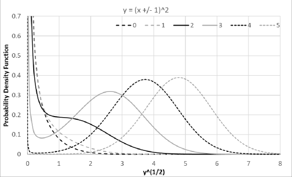
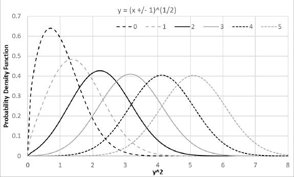
Viewed in the $f^{-1}(\tilde{y})$ coordinate, $\rho(\tilde{y},y,\delta y)$ is $\rho(\tilde{x},x,\delta x)$ modulated by $\frac{d\tilde{x}}{d\tilde{y}}=1/f^{(1)}_{x}$ , in which $f^{(1)}_{x}$ is the first derivative of $f(x)$ to $x$ . A distributional zero of the uncertainty distribution happens when $f^{(1)}_{x}=\infty\rightarrow\rho(\tilde{y},y,\delta y)=0$ , while a distributional pole happens when $f^{(1)}_{x}=0\rightarrow\rho(\tilde{y},y,\delta y)=\infty$ . Zeros and poles provides the strongest local modulation to $\rho(\tilde{x},x,\delta x)$ :

•

If $\tilde{y}=\alpha+\beta\tilde{x}$ , the result distribution is same as the original distribution, as $\rho(\tilde{y},y,\delta y)=\rho(\tilde{y},\alpha+\beta x,\beta\delta x)$ [5]. A linear transformation generates neither distributional zero nor distributional pole according to Formula (2.2).
•

Figure 1 shows the probability density function for $(x\pm 1)^{2}$ according to Formula (2.3), which has a distributional pole at $x=0$ . $(0\pm 1)^{2}$ is the $\chi^{2}$ distribution [2]. At the distributional pole, the probability density function resembles a Delta distribution.
•

Figure 2 shows the probability density function for $\sqrt{x\pm 1}$ according to Formula (2.3), which has a distributional zero at $x=0$ . At the distributional zero, the probability density function is zero.

In both Figure 1 and 2, the result probability density function in the $\tilde{z}$ representation resembles the input distribution more when the mode of the distributions is further away from either distributional pole or distributional zero.

2.3 Statistical Taylor Expansion

Formula (2.2) gives the uncertainty distribution of an analytic function. However, normal scientific and engineering calculations usually do not care about the result distribution, but just few statistics of the result, such as the result mean and deviation [2][3]. Such simple statistics is the result of statistical Taylor expansion. The deviation $\delta x$ in statistical Taylor expansion is also referred to as uncertainty, which may or may not be the measured statistical deviation.

An analytic function $f(x)$ can be precisely calculated in a range by the Taylor series as shown in Formula (2.5). Formula (2.4) defines bounded momentum $\zeta(n)$ , in which $0<\varrho,\sigma$ are bounding factors. Using Formula (2.4), Formula (2.6) and (2.3) gives the mean $\overline{f(x)}$ and the variance $\delta^{2}f(x)$ for $f(x)$ , respectively. $\overline{f(x)}-f(x)$ is defined as the uncertainty bias which is the effect of the input uncertainty to the result value.

$\displaystyle\zeta(n)\equiv$	$\displaystyle\int_{x-\varrho\delta x}^{x+\sigma\delta x}\rho(\tilde{x},x,\delta x)d\tilde{x}=\int_{-\varrho}^{+\sigma}\tilde{z}^{n}\rho(\tilde{z})d\tilde{z};$	(2.4)
$\displaystyle f(x+\tilde{x})=$	$\displaystyle f(x+\tilde{z}\delta x)=\sum_{n=0}^{\infty}\frac{f^{(n)}_{x}}{n!}\tilde{z}^{n}(\delta x)^{n};$	(2.5)
$\displaystyle\overline{f(x)}=$	$\displaystyle\int_{-\varrho}^{+\sigma}f(x+\tilde{x})\rho(\tilde{x},x,\delta x)d\tilde{x}=f(x)+\sum_{n=1}^{\infty}(\delta x)^{n}\frac{f^{(n)}_{x}}{n!}\zeta(n);$	(2.6)
$\displaystyle\delta^{2}f(x)=$	$\displaystyle\overline{(f(x)-\overline{f(x)})^{2}}=\overline{f(x)^{2}}-\overline{f(x)}^{2}$
	$\displaystyle=\sum_{n=1}^{\infty}(\delta x)^{n}\sum_{j=1}^{n-1}\frac{f^{(j)}_{x}}{j!}\frac{f^{(n-j)}_{x}}{(n-j)!}\big{(}\zeta(n)-\zeta(j)\zeta(n-j)\big{)};$	(2.7)

Due to uncorrelated uncertainty assumption, Formula (2.9) and (2.3) calculate the mean and variance of Taylor expansion in Formula (2.8), in which $\zeta_{x}(m)$ and $\zeta_{y}(n)$ are the variance momenta for $x$ and $y$ , respectively:

	$\displaystyle f(x+\tilde{x},y+\tilde{y})=\sum_{m=0}^{\infty}\sum_{n=0}^{\infty}\frac{f^{(m,n)}_{(x,y)}}{m!n!}\tilde{x}^{m}\tilde{y}^{n};$	(2.8)
$\displaystyle\overline{f(x,y)}=$	$\displaystyle\int\int f(x+\tilde{x},y+\tilde{y})\rho(\tilde{x},x,\delta x)\rho(\tilde{y},y,\delta y)\;d\tilde{x}d\tilde{y}$	(2.9)
$\displaystyle=$	$\displaystyle\sum_{m=0}^{\infty}\sum_{n=0}^{\infty}(\delta x)^{m}(\delta y)^{n}\frac{f^{(m,n)}_{(x,y)}}{m!\;n!}\zeta_{x}(m)\zeta_{y}(n);$
$\displaystyle\delta^{2}f(x,y)=$	$\displaystyle\sum_{m=1}^{\infty}\sum_{n=1}^{\infty}(\delta x)^{m}(\delta y)^{n}\sum_{i=0}^{m}\sum_{j=0}^{n}\frac{f^{(i,j)}_{(x,y)}}{i!\;j!}\frac{f^{(m-i,n-j)}_{(x,y)}}{(m-i)!\;(n-j)!}$
	$\displaystyle\;\;\;\;\;\;\;\;\;\;\;\;\;\;\;\;\;\;\;\;\;\;\;\;\big{(}\zeta_{x}(m)\zeta_{y}(n)-\zeta_{x}(i)\zeta_{x}(m-i)\;\zeta_{y}(j)\zeta_{y}(n-j)\big{)};$	(2.10)

Although Formula (2.3) is only for 2-dimensional, it can be extended easily to any dimensional.

2.4 Statistical Bounding

When the bounding factors $\varrho$ and $\sigma$ are limited, Formula (2.4) provides statistical bounding $\tilde{x}\in[x-\varrho\delta x,x+\sigma\delta x]$ . The probability $\epsilon$ for $\tilde{x}\not\in[x-\varrho\delta x,x+\sigma\delta x]$ is defined as bounding leakage.

2.5 Bounding Symmetry and Asymptote

A bounding $[x-\varrho\delta x,x+\sigma\delta x]$ is mean-preserving if $\zeta(1)=0$ , which has the same mean as the unbounded distribution. To achieve mean-preserving, $\sigma$ determines $\varrho$ . With mean-preserving bounding, Formula (2.11) and (2.12) give the result for $x\pm y$ , while Formula (2.13) and (2.14) give the result for $xy$ :

$\displaystyle\overline{x\pm y}$	$\displaystyle=x\pm y;$	(2.11)
$\displaystyle\delta^{2}(x\pm y)$	$\displaystyle=\zeta_{x}(2)(\delta x)^{2}+\zeta_{y}(2)(\delta y)^{2};$	(2.12)
$\displaystyle\overline{xy}$	$\displaystyle=xy;$	(2.13)
$\displaystyle\delta^{2}(xy)$	$\displaystyle=\zeta_{x}(2)(\delta x)^{2}y^{2}+x^{2}\zeta_{y}(2)(\delta y)^{2}+\zeta_{x}(2)(\delta x)^{2}\zeta_{y}(2)(\delta y)^{2};$	(2.14)

For any input distribution $\rho(\tilde{x},x,\delta x)$ symmetric around its mean $x$ , any $[x-\sigma\delta x,x+\sigma\delta x]$ bounding has property $\zeta(2n+1)=0$ , which simplifies statistical Taylor expansion further.

Empirically, as Formula (2.15), (2.18), and (2.23) will demonstrate, when $n\rightarrow+\infty$ , $\zeta(n)\rightarrow\sigma^{n}/n$ .

2.5.1 Uniform Input Uncertainty

For uniform distribution, the bounding factor is $\sigma=\sqrt{3}$ , and the bounding leakage $\epsilon=0$ . According to Formula (2.15), $\zeta(2n)=(\sqrt{3})^{2n}/(2n+1)$ while $\zeta(2n+1)=0$ .

\int_{-\sqrt{3}\delta x}^{+\sqrt{3}\delta x}\frac{1}{2\sqrt{3}\delta x}\tilde{x}^{2n}d\tilde{x}=(\delta x)^{2n}\frac{(\sqrt{3})^{2n}}{2n+1};

(2.15)

2.5.2 Gaussian Input Uncertainty

The central limit theorem converges other distributions toward Gaussian [5] after addition and subtraction, and such convergence is fast [1]. In a digital computer, multiplication is implemented as a series of shifts and additions, division is implemented as a series of shifts and subtractions, and general function is calculated as addition of expansion terms [8][9]. This is why in general an uncertainty without bounds is assumed to be Gaussian distributed [2][3][5].

For Gaussian uncertainty input, $\zeta(2n+1)=0$ .

If $\sigma=\infty$ , $\zeta(2n)=(2n-1)!!$ , which causes Formula (2.30) for $\log(x\pm\delta x)$ and Formula (2.33) for $(x\pm\delta x)^{c}$ to diverge. When $\sigma$ has an upper bound, Formula (2.4) becomes Formula (2.16):

$\displaystyle\zeta(2n)=$	$\displaystyle 2N(\sigma)\sigma^{2n}\sum_{j=1}^{\infty}\sigma^{2j-1}\frac{(2n-1)!!}{(2n-1+2j)!!};$	(2.16)
$\displaystyle=$	$\displaystyle(2n-1)\zeta(\sigma,2n-2)-2N(\sigma)\sigma^{2n-1};$	(2.17)
	$\displaystyle\sigma^{2}\ll 2n:\;\;\;\zeta(2n)\simeq 2N(\sigma)\frac{\sigma^{2n+1}}{2n+1};$	(2.18)

•

For small $2n$ , $\zeta(2n)$ can be approximated by $\zeta(2n)=(2n-1)!!$ according to Formula (2.17). When $\sigma=5,n<5$ , $\left|1-\eta(2n)/(2n-1)!!\right|<10^{-3}$ .
•

For large $2n$ , Formula (2.16) reduces to Formula (2.18), which shows that $\zeta(2n)$ increases slower than $\sigma^{2n}$ for increasing $2n$ .

Formula (2.19) gives the bounding leakage $\epsilon$ , in which $\xi(z)$ is the cumulative density function for Normal distribution [5].

\epsilon=2-2\xi(\frac{1}{2}+\sigma);

(2.19)

2.5.3 An Input Uncertainty with Limited Range

Formula (2.20) shows a distribution density function with $\tilde{x}\in[0,+\infty)$ , whose bounding range $[\varrho\lambda,\sigma\lambda]$ satisfying $0<\varrho<1<\sigma$ . Formula (2.21) shows its mean-preserving equation. Formula (2.22) shows its bounded momentum. Formula (2.23) shows its asymptote. Formula (2.24) shows its bounding leakage.

$\displaystyle\rho(\tilde{x},x,\delta x)$	$\displaystyle=\frac{\tilde{x}}{\lambda^{2}}e^{-\frac{\tilde{x}}{\lambda}};\;\;\;x=2\lambda;\;\;\;\delta^{2}x=2\lambda^{2};$	(2.20)
	$\displaystyle e^{-\varrho}\varrho^{2}=e^{-\sigma}\sigma^{2};$	(2.21)
$\displaystyle\zeta(n)$	$\displaystyle=(n+1)!\left(e^{-\varrho}\sum_{j=0}^{n+1}\frac{\varrho^{j}}{j!}-e^{-\sigma}\sum_{j=0}^{n+1}\frac{\sigma^{j}}{j!}\right);$	(2.22)
	$\displaystyle\lim_{n\rightarrow+\infty}\zeta(n)=\frac{\sigma^{n+2}}{n+2}e^{-\sigma};$	(2.23)
$\displaystyle\epsilon$	$\displaystyle=1-e^{-\varrho}+e^{-\sigma};$	(2.24)

2.6 One Dimensional Examples

Formula (2.26) and (2.27) give the mean and variance for $e^{x}$ , respectively:

	$\displaystyle e^{x+\tilde{x}}=e^{x}\sum_{n=0}^{\infty}\frac{\tilde{x}^{n}}{n!};$	(2.25)
$\displaystyle\frac{\overline{e^{x}}}{e^{x}}$	$\displaystyle=1+\sum_{n=1}^{\infty}(\delta x)^{n}\zeta(2n)\frac{1}{n!};$	(2.26)
$\displaystyle\frac{\delta^{2}e^{x}}{(e^{x})^{2}}$	$\displaystyle=\sum_{n=2}^{\infty}(\delta x)^{n}\sum_{j=1}^{n-1}\frac{\zeta(n)-\zeta(j)\zeta(n-j)}{j!\;(n-j)!};$	(2.27)

Formula (2.29) and (2.30) give the mean and variance for $\log(x)$ , respectively:

	$\displaystyle\log(x+\tilde{x})-\log(x)=\log(1+\frac{\tilde{x}}{x})=\sum_{j=1}^{\infty}\frac{(-1)^{j+1}}{j}\frac{\tilde{x}^{j}}{x^{j}};$	(2.28)
$\displaystyle\overline{\log(x)}$	$\displaystyle=\log(x)+\sum_{n=1}^{+\infty}P(x)^{n}\frac{(-1)^{n+1}\zeta(n)}{n};$	(2.29)
$\displaystyle\delta^{2}\log(x)$	$\displaystyle=\sum_{n=2}^{+\infty}P(x)^{n}\sum_{j=1}^{n-1}\frac{\zeta(n)-\zeta(j)\zeta(n-j)}{j(n-j)};$	(2.30)

Formula (2.32) and (2.33) give the mean and variance for $x^{c}$ , respectively:

	$\displaystyle(x+\tilde{x})^{c}=x^{c}(1+\frac{\tilde{x}}{x})^{c}=x^{c}+x^{c}\sum_{n=1}^{\infty}\frac{\tilde{x}^{n}}{x^{n}}\begin{pmatrix}c\\ n\end{pmatrix};\;\;\;\begin{pmatrix}c\\ n\end{pmatrix}\equiv\frac{\prod_{j=0}^{n-1}(c-j)}{n!};$	(2.31)
$\displaystyle\frac{\overline{x^{c}}}{x^{c}}$	$\displaystyle=1+1\sum_{n=1}^{\infty}P(x)^{n}\zeta(n)\begin{pmatrix}c\\ n\end{pmatrix};$	(2.32)
$\displaystyle\frac{\delta^{2}x^{c}}{(x^{c})^{2}}$	$\displaystyle=\sum_{n=2}^{\infty}P(x)^{n}\sum_{j=1}^{n-1}\begin{pmatrix}c\\ j\end{pmatrix}\begin{pmatrix}c\\ n-j\end{pmatrix}\big{(}\zeta(n)-\zeta(j)\zeta(n-j)\big{)};$	(2.33)

Formula (2.35) and (2.36) give the mean and variance for $\sin(x)$ , respectively:

$\displaystyle\sin(x+\tilde{x})$	$\displaystyle=\sum_{n=0}^{\infty}\eta(n,x)\frac{\tilde{x}^{n}}{n!};\;\;\;\eta(n,x)\equiv\begin{cases}n=4j:\;\;\;sin(x);\\ n=4j+1:\;\;\;cos(x);\\ n=4j+2:\;\;\;-sin(x);\\ n=4j+3:\;\;\;-cos(x);\end{cases}$	(2.34)
$\displaystyle\overline{\sin(x)}=$	$\displaystyle\sin(x)+\sum_{n=1}^{\infty}(\delta x)^{n}\eta(n,x)\frac{\zeta(n)}{n!};$	(2.35)
$\displaystyle\delta^{2}\sin(x)=$	$\displaystyle\sum_{n=2}^{\infty}(\delta x)^{n}\sum_{j=1}^{n-1}\frac{\eta(j,x)\eta(n-j,x)}{j!(n-j)!}\big{(}\zeta(n)-\zeta(j)\zeta(n-j)\big{)};$	(2.36)

The result variance in statistical Taylor expansion shows the nature of the calculation, such as $\delta x\rightarrow P(e^{x})$ , $\delta x\rightarrow\delta\sin(x)$ , $P(x)\rightarrow P(x^{c})$ , and $P(x)\rightarrow\delta\log(x)$ .

2.7 Dependency Tracing

$\displaystyle\delta^{2}(f+g)=$	$\displaystyle\delta^{2}f+\delta^{2}g+2(\overline{fg}-\overline{f}\overline{g});$	(2.37)
$\displaystyle\delta^{2}(fg)=$	$\displaystyle\overline{f^{2}g^{2}}-\overline{fg}^{2};$	(2.38)
$\displaystyle\delta^{2}f(g)=$	$\displaystyle\overline{f(g)^{2}}-\overline{f(g)}^{2};$	(2.39)
$\displaystyle\delta^{2}(c_{1}f+c_{0})=$	$\displaystyle c_{1}^{2}\delta^{2}f;$	(2.40)

When all the inputs obey the uncorrelated uncertainty assumption, statistical Taylor expansion traces dependency in the intermediate steps. For example:

•

Formula (2.37) shows $\delta^{2}(f+g)$ , whose dependence tracing can be demonstrated by $\delta^{2}(f-f)=0$ , and $\delta^{2}(f(x)+g(y))=\delta^{2}f+\delta^{2}g$ , with the latter corresponding to Formula (2.12). Formula (• ‣ 2.7) shows that Formula (2.3) uses Formula (2.37) between any two terms in the Taylor expansion of Formula (2.5).

		$\displaystyle\zeta(2n+1)=0:$
		$\displaystyle\;\;\;\delta^{2}\left(\frac{f^{(m)}_{x}\tilde{x}^{m}}{m!}+\frac{f^{(n)}_{x}\tilde{x}^{n}}{n!}\right)=(\delta x)^{2m}(\frac{f^{(m)}_{x}}{m!})^{2}\eta(2m)+(\delta x)^{2n}(\frac{f^{(n)}_{x}}{n!})^{2}\eta(2n)$
		$\displaystyle\;\;\;\;\;\;\;\;\;\;\;\;+2(\delta x)^{m+n}\left(\frac{f^{(m)}_{x}f^{(n)}_{x}}{m!\;n!}\eta(m+n)-\frac{f^{(m)}_{x}}{m!}\eta(m)\;\frac{f^{(n)}_{x}}{n!}\eta(n)\right);$

•

Formula (2.38) shows $\delta^{2}(fg)$ , whose dependence tracing can be demonstrated by $\delta^{2}(f/f)=0$ , $\delta^{2}(ff)=\delta^{2}f^{2}$ , and $\delta^{2}(f(x)g(y))=\overline{f}^{2}(\delta^{2}g)+(\delta^{2}f)\overline{g}^{2}+(\delta^{2}f)(\delta^{2}g)$ , with the latter corresponding to Formula (2.14).
•

Formula (2.39) shows $\delta^{2}f(g(x))$ , whose dependence tracing can be demonstrated by $\delta^{2}(f^{-1}(f))=(\delta x)^{2}$ .
•

Formula (2.40) shows the variance of linear transformation of a function, which can be applied to Formula (2.37) and (2.38) for more generic dependency tracing.

Variance arithmetic uses dependency tracing to guarantee that the result mean and variance fit statistics. Dependency tracing comes with a price: variance calculation is generally more complex than value calculation, and it has narrow convergence range for the input variables. Dependency tracing also implies that the result of statistical Taylor expansion should not be path dependent.

2.8 Traditional Execution and Dependency Problem

Dependency tracing requires an analytic solution to apply Taylor expansion for the result mean and variance, such as using Formula (2.6), (2.3), (2.9), and (2.3). It conflicts with traditional numerical executions on analytic functions:

•

Traditionally, using intermediate variables is a widespread practice. But it upsets dependency tracing through variable usage.
•

Traditionally, conditional executions are used to optimize numerical executions and to minimize rounding errors, such as the Gaussian elimination to minimize floating-point rounding errors for matrix inversion [37]. Unless required by mathematics such as for the definition of identity matrix, conditional executions need to be removed for dependency tracing, e.g., Gaussian elimination needs to be replaced by direct matrix inversion as described in Section 6.
•

Traditionally, approximations on the result values are carried out during executions. Using statistical Taylor expansion, Formula (2.3) shows that the variance converges slower than that of the value in Taylor expansion, so that the target of approximation should be more on the variance. Section 6 provides an example of first order approximation on calculating matrix determinant.
•

Traditionally, results from math library functions are trusted blindly down to every bit. As shown in Section 8, statistical Taylor expansion can now illuminate the numerical errors in math library functions, and it demands these functions to be recalculated with uncertainty as part of the output.
•

Traditionally, an analytic expression can be broken down into simpler and independent arithmetic operations of negation, addition, multiplication, division, and etc ⁴⁴4Sometimes square root is also regarded as an arithmetic operation.. But such approach causes the dependency problem in both floating-point arithmetic and interval arithmetic. It also causes the dependency problem in statistical Taylor expansion also. For example, if $x^{2}-x$ is calculated as $x^{2}-x$ , $x(x-1)$ , and $(x-\frac{1}{2})^{2}-\frac{1}{4}$ , only $(x-\frac{1}{2})^{2}-\frac{1}{4}$ gives the correct result, while the other two give wrong results for wrong independence assumptions between $x^{2}$ and $x$ , or between $x-1$ and $x$ , respectively.
•

Traditionally, a large calculation may be broken into sequential steps, such as calculating $f(g(x))$ as $f(y)|_{y=g(x)}$ . But this method no longer works in statistical Taylor expansion due to dependency tracing of $g(x)$ inside $f(g(x))$ , e.g., $\overline{f(g(x))}\neq\overline{f(y)|_{y=g(x)}}$ and $\delta^{2}f(g(x))\neq\delta^{2}f(y)|_{y=g(x)}$ . $f(y)|_{y=g(x)}$ is path-dependent, e.g., $\overline{(\sqrt{x})^{2}}>\overline{\sqrt{x^{2}}}$ and $\delta^{2}(\sqrt{x})^{2}>\delta^{2}\sqrt{x^{2}}$ .

Dependency tracing gets rid of almost all freedoms in the traditional numerical executions, as well as the associated dependence problems. All traditional numerical algorithms need to be reexamined or reinvented for statistical Taylor expansion.

3 Variance Arithmetic

Variance arithmetic implements statistical Taylor expansion, by adding practical assumptions.

3.1 Choices of Bounding Factors

For discussion simplicity, only Gaussian input uncertainty will be considered in this paper. For Gaussian input uncertainty, when $\sigma=5$ , $\epsilon=5.73\times 10^{-7}$ according to Formula (2.19), which is small enough for most applications. $\sigma=5$ is also a golden standard to assert a negative result [3]. Thus, $\sigma=5$ in variance arithmetic for Gaussian input uncertainty.

3.2 Low-Order Approximation

When $\sigma=5,n<5$ , Formula (2.27), and (2.30) can be simplified as Formula (3.1), and (3.2), respectively.

	$\displaystyle\frac{\delta^{2}e^{x}}{(e^{x})^{2}}\simeq$	$\displaystyle(\delta x)^{2}+\frac{3}{2}(\delta x)^{4}+\frac{7}{6}(\delta x)^{6}+\frac{5}{8}(\delta x)^{8}+o((\delta x)^{10});$		(3.1)
	$\displaystyle\delta^{2}\log(x)\simeq$	$\displaystyle P(x)^{2}+P(x)^{4}\frac{9}{8}+P(x)^{6}\frac{119}{24}+P(x)^{8}\frac{991}{32}+o(P(x)^{10});$		(3.2)

When $\sigma=5,n<5$ , Formula (2.33), and (2.36) can be simplified as Formula (3.2), (3.2), respectively.

$\displaystyle\frac{\delta^{2}x^{c}}{(x^{c})^{2}}\simeq$	$\displaystyle c^{2}P(x)^{2}+\frac{3}{2}c^{2}(c-1)(c-\frac{5}{3})P(x)^{4}$
	$\displaystyle+\frac{7}{6}c^{2}(c-1)(c-2)^{2}(c-\frac{16}{7})P(x)^{6}+o(P(x)^{8});$	(3.3)
$\displaystyle\delta^{2}\sin(x)\simeq$	$\displaystyle(\delta x)^{2}\cos(x)^{2}-(\delta x)^{4}(\cos(x)^{2}\frac{3}{2}-\frac{1}{2})$
	$\displaystyle+(\delta x)^{6}(\cos(x)^{2}\frac{7}{6}-\frac{1}{2})-(\delta x)^{8}(\cos(x)^{2}\frac{5}{8}-\frac{7}{24})+o((\delta x)^{10});$	(3.4)

Formula (3.5), (3.7), and (3.9) are special cases for Formula (2.32). Formula (3.6), (3.8), and (3.10) are special cases for Formula (3.2).

$\displaystyle\overline{x^{2}}\simeq$	$\displaystyle x^{2}+(\delta x)^{2};$	(3.5)
$\displaystyle\delta^{2}x^{2}\simeq$	$\displaystyle 4x^{2}(\delta x)^{2}+2(\delta x)^{4};$	(3.6)
$\displaystyle\frac{\overline{\sqrt{x}}}{\sqrt{x}}\simeq$	$\displaystyle 1-\frac{1}{8}P(x)^{2}-\frac{15}{128}P(x)^{4}-\frac{315}{1024}P(x)^{6}+o(P(x)^{8});$	(3.7)
$\displaystyle\frac{\delta^{2}\sqrt{x}}{(\sqrt{x})^{2}}\simeq$	$\displaystyle\frac{1}{4}P(x)^{2}+\frac{7}{32}P(x)^{4}+\frac{75}{128}P(x)^{6}+o(P(x)^{8});$	(3.8)
$\displaystyle\frac{\overline{1/x}}{1/x}\simeq$	$\displaystyle 1+P(x)^{2}+3P(x)^{4}+15P(x)^{6}+o(P(x)^{8});$	(3.9)
$\displaystyle\frac{\delta^{2}1/x}{(1/x)^{2}}\simeq$	$\displaystyle P(x)^{2}+8P(x)^{4}+69P(x)^{6}+o(P(x)^{8});$	(3.10)

3.3 Expansion Calculation

Due to digital limitation of conventional floating-point representation, $\zeta(2n)$ can only be calculated to $2n<442$ before becoming infinitive, Thus, variance arithmetic has different convergence rule from its counterpart of Taylor expansion of precise variable. In variance arithmetic, an infinitive expansion (including Taylor expansion) can fail for the following reasons: not monotonic, not stable, not positive, not finite, and not reliable.

3.3.1 Convergent

The necessary condition for the expansion to converge is that the absolute values of its terms decrease monotonically with increasing $2n$ when $2n$ is sufficiently large. To judge for the convergence of Formula (2.3) with limited expansion, the last $20$ terms of the expansion is required to be monotonically and absolutely decreasing, so that the chance of the expansion to absolutely increase is only $2^{-20}=9.53\;10^{-7}$ . Otherwise, the result is invalidated as not monotonic.

According to Formula (3.3.1), the condition for Formula (2.30) for $\log(x\pm\delta x)$ to converge is $P(x)\leq 1/\sigma=1/5$ , which is confirmed numerically by $\log(x|pm\delta x)$ as $P(x)\lesssim 0.20088$ . Beyond the upper bound $P(x)$ , the expansion is not monotonic. Variance arithmetic rejects the distributional zero of $\log(0)$ inside the range of $[x-\delta x,x+\delta x]$ statistically due to the divergence of Formula (2.30) mathematically, with $\zeta(2n)$ as the connection of these two worlds.

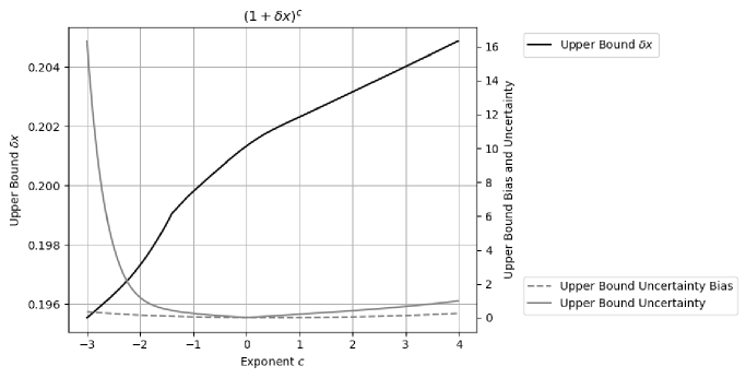
According to Formula (3.3.1), except when c is a nature number, Formula (2.33) for $(x\pm\delta x)^{c}$ converges near $P(x)\simeq 1/\sigma=1/5$ , with the upper bound $P(x)$ increasing with $c$ . This is confirmed approximately by Figure 3. Beyond the upper bound $P(x)$ , the expansion is not monotonic. Qualitatively, $\delta^{2}1/x$ converges slower than $\delta^{2}\sqrt{x}$ according to Formula (3.10) and (3.8).

$\delta x\lesssim 19.865$ for $e^{x\pm\delta x}$ regardless of $x$ , while $\delta\log(x\pm\delta x)\lesssim 0.213$ regardless of $x$ . Both are expected from the relation $\delta x\rightarrow P(e^{x})$ and $P(x)\rightarrow\delta\log(x)$ , respectively, as shown by Formula (2.27) and (2.30).

$\displaystyle\delta^{2}\log(x)\simeq$	$\displaystyle\sum_{n=1}^{+\infty}P(x)^{2n}\zeta(2n)\sum_{j=1}^{2n-1}\frac{1}{j}\frac{1}{2n-j}=\sum_{n=1}^{+\infty}P(x)^{2n}\zeta(2n)\frac{1}{n}\sum_{j=1}^{2n-1}\frac{1}{j};$
	$\displaystyle\lim_{n\rightarrow+\infty}P(x)^{2n}\zeta(2n)\frac{1}{n}\sum_{j=1}^{2n-1}\frac{1}{j}=P(x)^{2n}\sigma^{2n}\frac{2\log(2n)}{(2n)^{2}}\sigma N(\sigma);$	(3.11)
$\displaystyle\frac{\delta^{2}x^{c}}{(x^{c})^{2}}\simeq$	$\displaystyle\sum_{n=1}^{\infty}P(x)^{2n}\zeta(2n)\sum_{j=1}^{2n-1}\begin{pmatrix}c\\ j\end{pmatrix}\begin{pmatrix}c\\ 2n-j\end{pmatrix}\simeq\sum_{n=1}^{\infty}P(x)^{2n}\sigma^{2n}\frac{1}{2n}\sum_{j=1}^{2n-1}\begin{pmatrix}c\\ j\end{pmatrix}\begin{pmatrix}c\\ 2n-j\end{pmatrix};$
	$\displaystyle\frac{1}{2n}\sum_{j=1}^{2n-1}\begin{pmatrix}c\\ j\end{pmatrix}\begin{pmatrix}c\\ 2n-j\end{pmatrix}<\begin{cases}c<0:\left\|c\begin{pmatrix}c\\ 2n-1\end{pmatrix}\right\|<\frac{\left\|c\Gamma(c)\right\|}{(2n-1)!};\\ c>0:\begin{pmatrix}c\\ n\end{pmatrix}^{2}<1;\end{cases}$	(3.12)

3.3.2 Stable

Conventional condition to terminate an infinitive series numerically is when the residual of an expansion is less than the unit in the last place of the result [13]. In practice, the last expansion term usually proxies for the expansion residual if either the residual is known to be less than the last expansion term, or if the residual is difficult to calculate [13]. This method no longer works in variance arithmetic because the expansion is limited to $2n<442$ , and because the expansion result is no longer precise. The probability of an imprecie value $x\pm\delta x$ not equal $0$ is indicated by its z-statistic $\frac{|x|}{\delta x}$ [5]. If this probability is the bounding leakage $\epsilon$ , Formula (3.13) gives the corresponding upper bound $\tau$ for this z-statistic. Because variance arithmetic has already guaranteed that the expansion is absolutely and monotonically decreasing, if the absolute value of the last expansion term is more than $\tau$ -fold of the result uncertainty, the result is invalidated as not stable.

2\xi(\tau)=\epsilon:\;\;\;\tau\simeq\epsilon\frac{\sqrt{2\pi}}{2}=7.18\times 10^{-7};

(3.13)

When the Taylor expansion is calculated without enough expansion terms, e.g., if $(1\pm 0.193)^{-2}$ is calculated with only $60$ -term expansion, the result will be not stable.

3.3.3 Valid

At any order, if the expansion variance becomes negative, the result is invalidated as not positive.

The variance expansion can contain negative values, such as Formula (2.36) for $sin(x\pm\delta x)$ . Figure 4 shows that the upper bound $\delta x$ for $sin(x\pm\delta x)$ is periodic between $0.318\pi$ and $0.416\pi$ , which is nicely less than the periodicity $2\pi$ of $\sin(x)$ . Beyond the largest possible $\delta x$ , the expansion is invalidated as not positive in Figure 4.

3.3.4 Finite

If the result of Taylor expansion is not finite, the expansion is invalidated as not finite. This usually happens when the expansion diverges so that it is usually not the reason to bound $\delta x$ . For example $(1\pm 1)^{-2}$ has infinitive variance.

3.3.5 Reliable

While $\delta x$ specifies the uncertainty of $x$ , the calculated $\delta x$ itself can be imprecise. To guarantee $\delta x$ to be precise enough, during expansion, if the value of the variance is less than the $1/\sigma$ -fold of its uncertainty, the result is invalidated as not reliable.

Fortunately, being not reliable is rarely the reason to bound $\delta x$ .

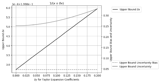
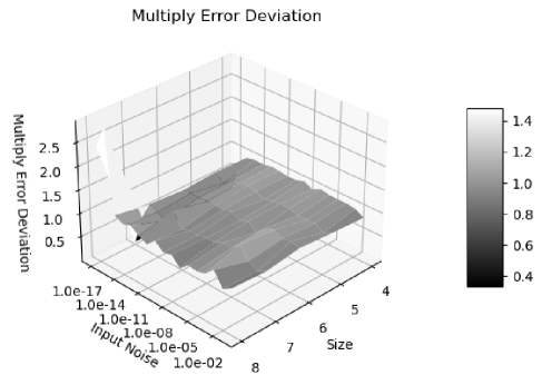
In Formula (2.5) for Taylor expansion, the coefficient $f^{(n)}_{x}/n!$ can be imprecise, whose uncertainties also contributes to the result variance. Figure 5 shows the upper bound $\delta x$ of $1/(1\pm\delta x)$ for different uncertainty $\delta y$ of Taylor expansion coefficients. It shows that the result upper bound uncertainty $\delta x=0.19980273+\delta y\times 16.1\;10^{-6}$ . In this example, such linear increase is extremely small. For discussion simplicity, the Taylor coefficient in Formula (2.5) is assumed to be precise in this paper.

3.3.6 Continuous

The result mean, variance and histogram of variance arithmetic are generally continuous in parameter space.

When $c$ is a nature number $n$ , Formula (2.33) has $n$ terms, so that $\delta x$ has no upper bound for $(x\pm\delta x)^{n}$ unless for not finite, such as Formula (3.6) for $(x\pm\delta x)^{2}$ . The result mean, variance and histogram of $(x\pm\delta x)^{c}$ are continuous around $c=n$ . Table 1 shows that the result of $(1\pm\delta x)^{n\pm d}$ is very close to that of $(1\pm\delta x)^{n}$ , even the former had upper bound for $\delta x$ , while the latter has not.

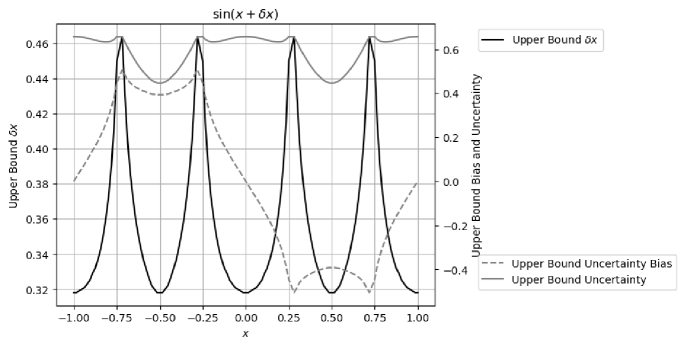
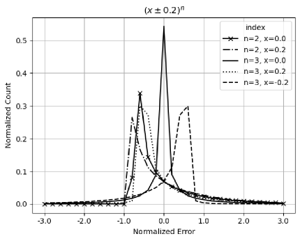
A statistical bounding range of variance arithmetic can include a distributional pole when an analytic function is defined around the distributional pole. The presence of such distributional poles does not cause any discontinuity of the result mean, variance, and histogram. Figure 7 shows the histograms of $(x\pm 0.2)^{n}$ when $x=0,-0.2,+0.2$ and $n=2,3$ .

•

When the second derivative is zero, the resulted distribution is symmetric two-sided Delta-like, such as when $n=3,x=0$ .
•

When the second derivative is positive, the resulted distribution is right-sided Delta-like, such as the $\chi^{2}$ distribution when $n=2,x=0$ , or when $n=2,x=\pm 0.2$ , or when $n=3,x=0.2$ .
•

When the second derivative is negative, the resulted distribution is left-sided Delta-like, such as when $n=3,x=-0.2$ , which is the mirror image of the distribution when $n=3,x=0.2$ .
•

In each case, the transition from $x=0$ to $x=0.2$ is continuous.

A statistical bounding range of variance arithmetic cannot include more than one distributional pole because the corresponding statistical Taylor expansion becomes not positive. One such example is $\sin(x)$ in Figure 4.

A statistical bounding range of variance arithmetic cannot include any distributional zero because the underlying analytic function is not continuous when its first derivative becomes infinitive.

$n\pm d$	$0\pm 10^{-6}$	$1\pm 10^{-6}$	$2\pm 10^{-6}$	$3\pm 10^{-6}$
Upper Bound $\delta x$	$0.2006$	$0.2014$	$0.2018$	$0.2020$
Value	$1\mp 2.155\;10^{-8}$	$1\pm 2.073\;10^{-8}$	$1.041\pm 6.065\;10^{-8}$	$1.122\pm 1.328\;10^{-7}$
Uncertainty	$0+2.127\;10^{-7}$	$0.201-1.358\;10^{-6}$	$0.407\pm 2.201\;10^{-7}$	$0.654\pm 2.784\;10^{-7}$

Table 1: The result value and uncertainty of

(1\pm\delta x)^{n\pm d}

(1\pm\delta x)^{n}

, in which

n

is a natural number,

0<d\ll 1

, and

\delta x

is the upper bound for

(1\pm\delta x)^{n\pm d}

3.4 Numerical Representation

Variance arithmetic uses a pair of 64-bit standard floating-point numbers to represent the value $x$ and the variance $(\delta x)^{2}$ of an imprecise value $x\pm\delta x$ .

The equivalent floating-point value of the least significant bit of significand of a floating-point value is defined as the least significant value ⁵⁵5The “least significant value” and “unit in the last place” are different in concept., which can be abbreviated as $LSV$ for simplicity.

When the uncertainty $\delta x$ is not specified initially:

•

For a 64-bit standard floating-point value: If the least $22$ bits of its significand are all $0$ , the value is precise, representing a 2’s fractional with a possibility no less than $1-2^{-20}=1-2.384\;10^{-7}$ ; Otherwise, it is imprecise with the uncertainty being $1/\sqrt{3}$ -fold of $LSV$ , because pure rounding error of round-to-nearest is uniformly distributed within half bit of the significand of the floating-point value [1].
•

For an integer value: If it is within the range of $[-2^{53}+1,+2^{53}-1]$ ⁶⁶6Including a hidden bit, the significand in the standard IEEE 64-bit floating-point representation is 53-bit., it has 0 as its uncertainty; Otherwise, it is first converted to a conventional floating-point value before converted to an imprecise value.

3.5 Tracking Rounding Error

Variance arithmetic can track rounding errors effectively without requiring additional rules.

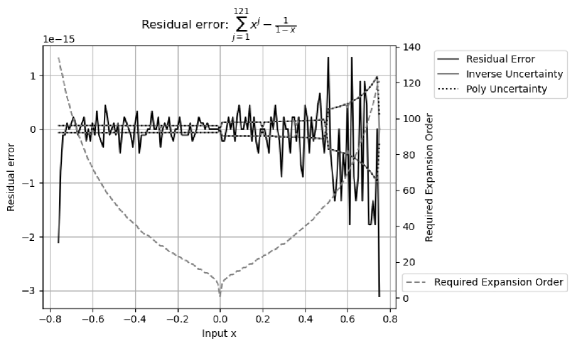
Figure 7 shows the residual error of $\sum_{j=0}^{121}x^{j}-\frac{1}{1-x}$ , in which the polynomial $\sum_{j=0}^{121}x^{j}$ is calculated using Formula (3.14), $\frac{1}{1-x}$ is calculated using Formula (2.31), and $x$ is initiated as a floating-point value. Because $\eta(2n)$ is limited to $2n\leq 242$ , Formula (3.14) for polynomial is limited to $N\leq 121$ , so that $\sum_{j=0}^{121}x^{j}$ has lower expansion order than that of $\frac{1}{1-x}$ . Figure 7 shows:

•

When $x\in[-0.73,0.75]$ , the required expansion order is no more than $121$ , so that the residual error is the calculation rounding error between $\sum_{j=0}^{121}x^{j}$ and $\frac{1}{1-x}$ . Detailed analysis shows that the max residual error is $4$ -fold of the $LSV$ of $\frac{1}{1-x}$ . The calculated uncertainty bounds the residual error nicely for all $x\in[-0.73,0.75]$ .
•

When $x\not\in[-0.74,+0.75]$ , such as when $x=-0.75,0.76$ , the required expansion order is more than $121$ , so that the residual error is caused by insufficient expansion order of $\sum_{j=0}^{121}x^{j}$ , and the residual error increases absolutely when $|x|\rightarrow 1$ , e.g., reaching $50$ when $x=0.98$ .

\sum_{j=0}^{N}c_{j}(x+\tilde{x})^{j}=\sum_{j=0}^{N}\tilde{x}^{j}\sum_{k=0}^{N-j}x^{k-j}c_{j+k}\begin{pmatrix}j+k\\ j\end{pmatrix};

(3.14)

3.6 Comparison

Two imprecise values can be compared statistically using the z-statistic [5] of their difference.

When the value difference is zero, the two imprecise values are equal. In statistics, such two imprecise values have $50\%$ possibility to be less than or greater to each other but no chance to be equal to each other [5]. In variance arithmetic, these two imprecise values are neither less nor greater than each other, so they are equal. In reality, the probability of two imprecise values equal exactly to each other is very low.

Otherwise, the standard z-statistic method [5] is used to judge whether they are equal, or less or more than each other. For example, the difference between $1.002\pm 0.001$ and $1.000\pm 0.002$ is $0.002\pm 0.00224$ , so that the z-statistic for the difference is $z=0.002/0.00224$ , and the probability for them to be not equal is $2\xi(|z|)=62.8\%$ , in which $\xi(z)$ is the cumulative density function for Normal distribution [5]. If the threshold probability of not equality is $50\%$ , $1.000\pm 0.002<1.002\pm 0.001$ . Instead of using the threshold probability, the equivalent bounding range for z can be used, such as $|z|\leq 0.67448975$ for the equal threshold probability of $50\%$ .

4 Verification of Statistical Taylor Expansion

4.1 Verification Methods and Standards

Verification of statistical Taylor expansion is done through the verification of variance arithmetic. Analytic functions or algorithms each with precisely known results are used to validate the result from variance arithmetic using the following statistical properties:

•

value error: as the difference between the numerical result and the corresponding known precise analytic result.
•

normalized error: as the ratio of a value error to the corresponding uncertainty.
•

error deviation: as the standard deviation of the normalized errors.
•

error distribution: as the histogram of the normalized errors.
•

uncertainty mean: as the mean of the result uncertainties.
•

uncertainty deviation: as the deviation of the result uncertainties.
•

error response: as the relation between the input uncertainties and the result uncertainties.
•

calculation response: as the relation between the amount of calculation and the result uncertainties.

One goal of calculation involving uncertainty is to precisely account for all input errors from all sources, to achieve ideal coverage. In the case of ideal coverage:

1.

The error deviation is exactly $1$ .
2.

The result error distribution should be Normal distribution when an imprecise value is expected, or Delta distribution when a precise value such as a true zero is expected.
3.

The error response fits the function, such as a linear error response is expected for a linear function.
4.

The calculation response fits the function, such as more calculations generally result in larger result uncertainties.

If the precise result is not known, according to Section 6, the result uncertainty distribution can be used to judge whether ideal coverage is achieved or not.

If instead, the input uncertainty is only correct for the input errors on the order of magnitude, the proper coverage is achieved when the error deviations are in the range of $[0.1,10]$ .

When an input contains unspecified errors, such as numerical errors of library functions, Gaussian or white noises of increasing deviations can be added to the input, until ideal coverage is reached. The needed minimal noise deviation gives a good estimation of the amount of unspecified input uncertainties. The existence of ideal coverage is a necessary verification if the application of Formula (2.3) or (2.3) has been applied correctly for the application. The input noise range for the idea coverage defines the ideal application range of input uncertainties.

Gaussian or white noises of specified deviations can also be added to the input to measure the error responses of a function.

4.2 Types of Uncertainties

There are five sources of result uncertainty for a calculation [1][2][13]:

•

input uncertainties,
•

rounding errors,
•

truncation errors,
•

external errors,
•

modeling errors.

The examples in this paper show that when the input uncertainty precision is $10^{-15}$ or larger, variance arithmetic can provide ideal coverage for input uncertainties.

Empirically, variance arithmetic can provide proper coverage to rounding errors, with the error deviations in the range of $[1/5,5]$ .

Section 3 shows that variance arithmetic uses $\tau$ -based rule for truncation error.

The external errors are the value errors which are not specified by the input uncertainties, such as the numerical errors in the library math functions. Section 8 studies the effect of $\sin$ and $\tan$ numerical errors [13]. It demonstrates that when the external errors are large enough, neither ideal coverage nor proper coverage can be achieved. It shows that the library functions need to be recalculated to have corresponding uncertainty attached to each value.

The modelling errors arise when an approximate analytic solution is used, or when a real problem is simplified to obtain the solution. For example, the predecessor of variance arithmetic [1] demonstrates that the discrete Fourier transformation is only an approximation for the mathematically defined continuous Fourier transformation. Conceptually, modeling errors originate from mathematics, so they are outside the domain for variance arithmetic.

4.3 Types of Calculations to Verify

Algorithms of completely different nature with each representative for its category are needed to test the generic applicability of variance arithmetic [1]. An algorithm can be categorized by comparing the amount of its input and output data as [1]:

•

application,
•

transformation,
•

generation,
•

reduction.

An application algorithm calculates numerical values from an analytic formula. Through Taylor expansion, variance arithmetic is directly applicable to analytic problems.

A transformation algorithm has about equal amounts of input and output data. The information contained in the data remains about the same after transforming. For reversible transformations, a unique requirement for statistical Taylor expansion is to recover the original input uncertainties after a round-trip transformation which is a forward followed by a reverse transformation. Discrete Fourier Transformation is a typical reversible transforming algorithm, which contains the same amount of input and output data, and its output data can be transformed back to the input data using essentially the same algorithm. A test of variance arithmetic using FFT algorithms is provided in Section 8.

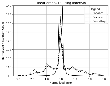
A generation algorithm has much more output data than input data. The generating algorithm codes mathematical knowledge into data, so there is an increase of information in the output data. Some generating algorithms are theoretical calculations which involve no imprecise input so that all result uncertainty is due to rounding errors. Section 9 demonstrates such an algorithm, which calculates a table of the sine function using trigonometric relations and two precise input data, $sin(0)=0$ and $sin(\pi/2)=1$ .

A reduction algorithm has much less output data than input data such as numerical integration and statistical characterization of a data set. Some information of the data is lost while other information is extracted during reducing. Conventional wisdom is that a reducing algorithm generally benefits from a larger input data set [5]. For example, discrete Fourier transformation was found to be unfaithful for continuous Fourier transformation [1].

5 Math Library Functions

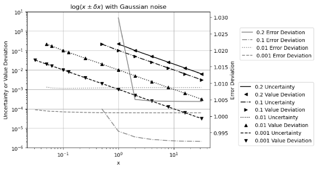
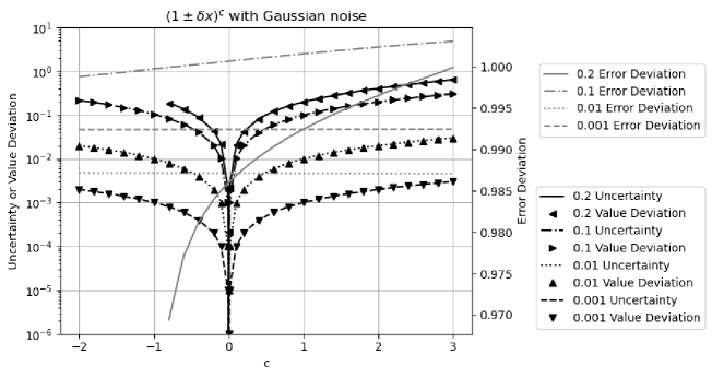
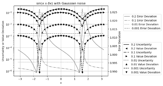
Formula (2.27), (2.30), (2.36), and (2.33) are tested by the corresponding math library functions exp, log, sin, and pow, respectively.

At each point $x$ for an input uncertainty $\delta x$ , the result uncertainty is calculated by variance arithmetic. The corresponding error deviation is obtained by sampling:

1.

Take $10000$ samples from either Gaussian noise or uniform distribution with $\delta x$ as the deviation, and construct $\tilde{x}$ which is $x$ plus the sampled noise.
2.

For each $\tilde{x}$ , use the corresponding library function to calculate the value error as the difference between using $\tilde{x}$ and using $x$ as the input.
3.

The value error is divided by the result uncertainty, as the normalized error.
4.

The standard deviation of the $10000$ normalized errors is the error deviation.
5.

In addition, for each of these tests, all value errors follow the same underlying distribution. The deviation of the value errors is defined as the value deviation, which the uncertainty should match.

5.1 Exponential

Figure 8 shows that the calculated uncertainties using Formula (2.27) agree very well with the measured value deviations for $e^{x+\delta x}$ . As a result, all error deviations are very close to $1$ , even though both the uncertainties and the value error deviations increase exponentially with $x$ and $\delta x$ .

5.2 Logarithm

$\log(x)$ has a distributional zero at $x=0$ so that all $log(x\pm\delta x)$ are rejected when $1/5<P(x)$ . Figure 9 shows that the calculated uncertainties using Formula (2.30) agree very well with the measured value deviations for $\log(x+\delta x)$ , and the result error deviations are very close to $1$ .

5.3 Power

Figure 10 shows that the calculated uncertainties of $(1\pm\delta x)^{c}$ using Formula (2.33) agree very well with the measured value deviations for $(1+\delta x)^{c}$ , with the error deviations close to $1$ .

5.4 Sine

Figure 11 shows that the calculated uncertainties using Formula (2.36) agree very well with the measured value deviations for $\sin(x+\delta x)$ . It also shows that $\delta^{2}\sin(x)$ has the same periodicity as $\sin(x)$ :

•

When $x=0$ , $\sin(x)\simeq x$ , so that $\delta^{2}\sin(x)\simeq(\delta x)^{2}$ .
•

When $x=\pi/2$ , $\sin(x)\simeq 1$ , so that $\delta^{2}\sin(x)\simeq 0$ .

$\sin(x)$ has distributional poles at $x=\pm\pi/2$ . Figure 12 shows that the error deviation for $\sin(x+\delta x)$ is $1$ except when $x=\pm\pi/2$ and $\delta x<10^{-8}$ , which agrees with the expected Delta distribution at $x=\pm\pi/2$ . In other places, the error deviations are very close to $1$ .

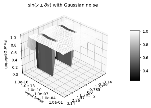
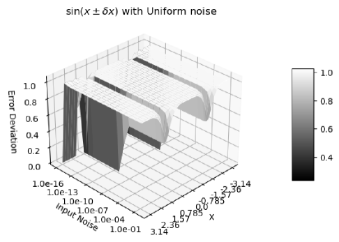
Figure 12 and Figure 13 both show the result uncertainty of $\sin(x+\delta x)$ vs the input $x$ and the input uncertainty $\delta x$ . In Figure 12, Gaussian noises are used, while in Figure 13, the input noises are uniformly distributed. The difference of Figure 12 and 13 shows that the uniform noise or white noise ⁷⁷7White noise is sampled from uniform distributed noise. is more local, while Gaussian noise has strong tail effect, so that the error deviation is much closer to $1$ for $\sin(\pm\pi/2+\delta x)$ when $\delta x>10^{-12}$ . In both cases, there is a clear transition at $\delta x=10^{-12}$ , which is caused by numerical errors in library $\sin(x)$ , as demonstrated in Section 8. For consistency, only Gaussian noises will be used for other analysis by default.

5.5 Numerical Errors for Library Functions

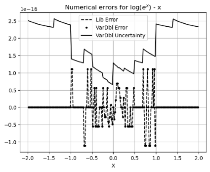
The combined numerical error of the library function $e^{x}$ and $\log(x)$ is calculated as $\log(e^{x})-x$ . Figure 14 shows that using either variance arithmetic or the conventional floating-point library functions results in the same value errors. The uncertainties of variance arithmetic bound the value errors effectively, resulting in an error deviation about $0.409$ when $|x|\leq 1$ . It looks suspicious when $|x|>1$ the value error is always $0$ in both calculations.

The numerical error of the library function $x^{p}$ is calculated as $(x^{p})^{1/p}-x$ . Figure 15 shows that the normalized errors are not specific to either $x$ or $p$ , resulting in an error deviation $0.548\pm 0.8$ .

The numerical errors of the library functions $\sin(x)$ , $\cos(x)$ , and $\tan(x)$ will be studied in detail later in Section 8.

5.6 Summary

Formula (2.27), (2.30), (2.33), and (2.36) give effective uncertainties for the corresponding library functions. With added noise larger than $10^{-15}$ , ideal coverage is achievable unless near a distributional pole where the deviation is $0$ . In non-ideal coverage cases, the error deviation is about $0.5$ so that proper coverage is achieved.

6 Matrix Inversion

6.1 Uncertainty Propagation in Matrix Determinant

Let vector $[p_{1},p_{2}\dots p_{n}]_{n}$ denote a permutation of the vector $(1,2\dots n)$ [37]. Let $\$[p_{1},p_{2}\dots p_{n}]_{n}$ denote the permutation sign of $[p_{1},p_{2}\dots p_{n}]_{n}$ [37]. Formula (6.1) defines the determinant of a $n$ -by- $n$ square matrix $\mathbf{M}$ with the element $x_{i,j},i,j=1\dots n$ [37]. The sub-determinant $M_{i,j}$ at index $(i,j)$ is formed by deleting the row $i$ and column $j$ of $M$ , whose determinant is given by Formula (6.2) [37]. Formula (6.3) holds for the arbitrary row index $i$ or the arbitrary column index $j$ [37].

$\displaystyle\|\mathbf{M}\|$	$\displaystyle\equiv\sum_{[p_{1}\dots p_{n}]_{n}}\$[p_{1}\dots p_{n}]_{n}\prod_{k=1\dots n}x_{k,p_{k}};$	(6.1)
$\displaystyle\|\mathbf{M}\|_{i,j}$	$\displaystyle\equiv\sum_{[p_{1}\dots p_{n}]_{n}}^{p_{i}=j}\$[p_{1}\dots p_{n}]_{n}\prod_{k=1\dots n}^{k\neq i}x_{k,p_{k}};$	(6.2)
$\displaystyle\|\mathbf{M}\|$	$\displaystyle=\sum_{j=1\dots n}\|\mathbf{M}_{i,j}\|x_{i,j}=\sum_{i=1\dots n}\|\mathbf{M}_{i,j}\|x_{i,j};$	(6.3)

Assuming $p_{1},p_{2}\in\{1\dots n\}$ , let $[p_{1},p_{2}]_{n}$ denote the length-2 unordered permutation which satisfies $p_{1}\neq p_{2}$ , and let $<p_{1},p_{2}>_{n}$ denote the length-2 ordered permutation which satisfies $p_{1}<p_{2}$ , and let ${<i_{1},i_{2}>}_{n}$ be an arbitrary ordered permutation ⁸⁸8An ordered permutation is a sorted combination.. Formula (6.3) can be applied to $M_{i,j}$ , as:

		$\displaystyle\|\mathbf{M}_{<i_{1},i_{2}>_{n},[j_{1},j_{2}]_{n}}\|\equiv\sum_{[p_{1}\dots p_{n}]_{n}}^{p_{i_{1}}=j_{1},p_{i_{2}}=j_{2}}\$[p_{1}\dots p_{n}]_{n}\prod_{k=1\dots n}^{k\not\in\{i_{1},i_{2}\}}x_{k,p_{k}};$		(6.4)
	$\displaystyle\|\mathbf{M}\|$	$\displaystyle=\sum_{j_{1}=1\dots n}x_{i_{1},j_{1}}\|\mathbf{M}_{i_{1},j_{1}}\|=\sum_{j_{1}=1\dots n}\sum_{j_{2}=1\dots n}^{j_{2}\neq j_{1}}\|\mathbf{M}_{<i_{1},i_{2}>_{n},[j_{1},j_{2}]_{n}}\|x_{i_{1},j_{1}}x_{i_{2},j_{2}};$		(6.5)

The definition of a sub-determinant can be extended to Formula (6.6), in which $m=1...n$ . Formula (6.5) can be generalized as Formula (6.7), in which $<i_{1}\dots i_{m}>_{n}$ is an arbitrary ordered permutation. The $(n-m)$ -by- $(n-m)$ matrix in $|\mathbf{M}_{<i_{1}\dots i_{m}>_{n}[j_{1}\dots j_{m}]_{n}}|$ is obtained by deleting the rows in $\{i_{1}\dots i_{m}\}$ and the columns in $\{j_{1}\dots j_{m}\}$ . This leads to Formula (6.8) ⁹⁹9 $\left||\mathbf{M}|\right|$ in Formula (6.8) means absolute value of determinant..

	$\displaystyle\|\mathbf{M}_{<i_{1}\dots i_{m}>_{n},[j_{1}\dots j_{m}]_{n}}\|\equiv\sum_{[p_{1}\dots p_{n}]_{n}}^{k\in\{i_{1}\dots i_{m}\}:p_{k}=j_{k}}\$[p_{1}\dots p_{n}]_{n}\prod_{k=1\dots n}^{k\not\in\{i_{1}\dots i_{m}\}}x_{k,p_{k}};$	(6.6)
$\displaystyle\|\mathbf{M}\|$	$\displaystyle=\sum_{{[j_{1}\dots j_{m}]}_{n}}\|\mathbf{M}_{<i_{1}\dots i_{m}>_{n},[j_{1}\dots j_{m}]_{n}}\|\prod_{k=1}^{m}x_{i_{k},j_{k}};$	(6.7)
	$\displaystyle\left\|\|\mathbf{M}_{<i_{1}\dots i_{m}>_{n},[j_{1}\dots j_{m}]_{n}}\|\right\|=\left\|\|\mathbf{M}_{<i_{1}\dots i_{m}>_{n},<j_{1}\dots j_{m}>_{n}}\|\right\|;$	(6.8)

Formula (6.9) give the Taylor expansion $|\widetilde{\mathbf{M}}|$ of $|\mathbf{M}|$ , which leads to Formula (6.10) and (6.11) for mean and variance of matrix determinant, respectively.

$\displaystyle\|\widetilde{\mathbf{M}}\|$	$\displaystyle=\sum_{[p_{1}\dots p_{n}]_{n}}\$[p_{1}\dots p_{n}]_{n}\prod_{i=1\dots n}(x_{i,p_{i}}+\tilde{x}_{i,p_{i}})$	(6.9)
	$\displaystyle=\sum_{m=0\dots n}\sum_{<i_{1}\dots i_{m}>_{n}}\sum_{[j_{1}\dots j_{m}]_{n}}\mathbf{M}_{<i_{1}\dots i_{m}>_{n},[j_{1}\dots j_{m}]_{n}}\prod_{i=1\dots m}^{i\in\{i_{1}\dots i_{m}\}}\tilde{x}_{i,p_{i}};$
$\displaystyle\overline{\|\mathbf{M}\|}$	$\displaystyle=\|\mathbf{M}\|;$	(6.10)
$\displaystyle\delta^{2}\|\mathbf{M}\|$	$\displaystyle=\sum_{m=1}^{n}\sum_{<i_{1}\dots i_{m}>_{n}}\sum_{[j_{1}\dots j_{m}]_{n}}\|\mathbf{M}_{<i_{1}\dots i_{m}>_{n},<j_{1}\dots j_{m}>_{n}}\|^{2}\prod_{k=1\dots n}^{i_{k}\in\{i_{1}\dots i_{m}\}}(\delta x_{i_{k},j_{k}})^{2};$	(6.11)

Formula (6.10) and (6.11) assume that the uncertainties of matrix elements are independent of each other. In contrast, for the special matrix in Formula (6.12), after applying Formula (2.9) and (2.3), Formula (6.13) and (6.14) give the result mean and variance, respectively.

$\displaystyle\|\mathbf{M}\|$	$\displaystyle=\left\|\begin{matrix}x,z,y\\ z,y,x\\ y,x,z\end{matrix}\right\|=3xyz-x^{3}-y^{3}-z^{3};$	(6.12)
$\displaystyle\overline{\|\mathbf{M}\|}$	$\displaystyle=\|\mathbf{M}\|-3x(\delta x)^{2}-3y(\delta y)^{2}-3z(\delta z)^{2};$	(6.13)
$\displaystyle\delta^{2}\|\mathbf{M}\|$	$\displaystyle=3(5x^{4}-12x^{2}yz+2xy^{3}+2xz^{3}+3y^{2}z^{2})(\delta x)^{2}$	(6.14)
	$\displaystyle+3(5y^{4}-12y^{2}xz+2yx^{3}+2yz^{3}+3x^{2}z^{2})(\delta y)^{2}$
	$\displaystyle+3(5z^{4}-12z^{2}xy+2zx^{3}+2zy^{3}+3x^{2}y^{2})(\delta z)^{2}$
	$\displaystyle+9(z^{2}+2xy)(\delta x)^{2}(\delta y)^{2}+9(y^{2}+xz)(\delta x)^{2}(\delta z)^{2}+9(x^{2}+2yx)(\delta y)^{2}(\delta z)^{2}$
	$\displaystyle+9(5x^{2}-2yz)(\delta x)^{4}+9(5y^{2}-2xz)(\delta y)^{4}+9(5z^{4}-2xy)(\delta z)^{4}$
	$\displaystyle+15(\delta x)^{6}+15(\delta y)^{6}+15(\delta z)^{6};$

6.2 Adjugate Matrix

The square matrix whose element is $(-1)^{i+j}|\mathbf{M}_{j,i}|$ is defined as the adjugate matrix[37] $\mathbf{M}^{A}$ to the original square matrix $\mathbf{M}$ . Let $\mathbf{I}$ be the identical matrix for $\mathbf{M}$ . Formula (6.15) and (6.16) show the relation of $\mathbf{M}^{A}$ and $\mathbf{M}$ [37].

	$\displaystyle\mathbf{M}\times\mathbf{M}^{A}$	$\displaystyle=\mathbf{M}^{A}\times\mathbf{M}=\|\mathbf{M}\|\mathbf{I};$		(6.15)
	$\displaystyle\|\mathbf{M}\|\mathbf{M}^{A}$	$\displaystyle=\|\mathbf{M}^{A}\|\mathbf{M};$		(6.16)

To test Formula (6.11):

1.

A matrix $\mathbf{M}$ is constructed using random integers uniformly distributed in the range of $[-2^{8},+2^{8}]$ , which has a distribution deviation of $2^{8}/\sqrt{3}$ . The integer arithmetic grantees that $|\mathbf{M}|$ , $\mathbf{M}^{A}$ , and $|\mathbf{M}^{A}|$ are precise.
2.

Gaussian noises of predefined levels are added to $\mathbf{M}$ , to construct a $\widetilde{\mathbf{M}}$ which contains imprecise values. Variance arithmetic is used to calculate $|\widetilde{\mathbf{M}}|$ , $\widetilde{\mathbf{M}}^{A}$ , and $|\widetilde{\mathbf{M}}^{A}|$ . For example, to construct a $\widetilde{\mathbf{M}}$ with $10^{-3}$ input noise precision, the deviation of the Gaussian noise is $10^{-3}\times 2^{8}/\sqrt{3}$ .
3.

The difference between $\widetilde{\mathbf{M}}^{A}$ and $\mathbf{M}^{A}$ defines the Adjugate Test. Figure 16 shows that the result uncertainties increase exponentially with both the input noises and the matrix size, while Figure 17 shows that the ideal coverage is achieved for the input precision greater than $10^{-16}$ .
4.

Formula (6.15) defines the Forward Test. Figure 18 shows that the differences of the two sides of Formula (6.15) is true zero, confirming Formula (6.15) in the context of ideal converge in Figure 17.
5.

Formula (6.16) defines the Roundtrip Test. Similarly, Figure 19 shows that Formula (6.16) is strictly observed for the idea coverage.

The existence of ideal coverage validates Formula (6.11).

6.3 Floating Point Rounding Errors

Error Deviation	Input Noise Precision
Matrix Size	$0$	$10^{-17}$	$10^{-16}$	$10^{-15}$
$4$	$0$	$0$	$0.68$	$1.03$
$5$	$0$	$0.003$	$0.60$	$0.96$
$6$	$0$	$0.006$	$0.80$	$1.04$
$7$	$0$	$0.083$	$1.05$	$1.05$
$8$	$4.62$	$3.91$	$3.01$	$1.01$

Table 2: The error deviation as a function of matrix size and input noise precision for

\mathbf{M}^{A}

in which

\mathbf{M}

is generated by random integers between

[-2^{8},+2^{8}]

. The measured error deviations change slightly for different runs.

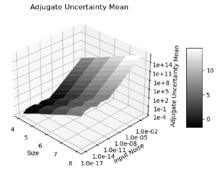
The significand of the conventional floating-point representation [9] has $53$ -bit resolution, which is equivalent to $10^{-16}$ . Adding noise below this level will not change the value of a conventional floating-point value, so the result uncertainties are caused by the round errors in the floating-point calculations.

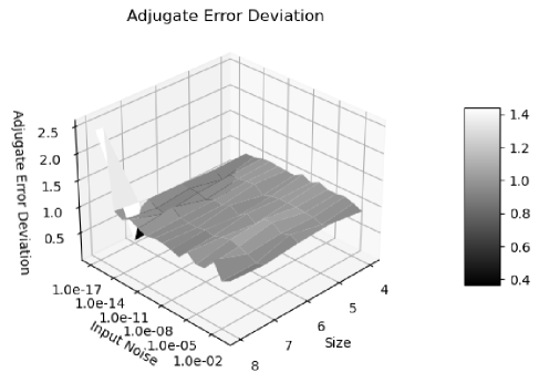
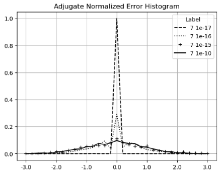
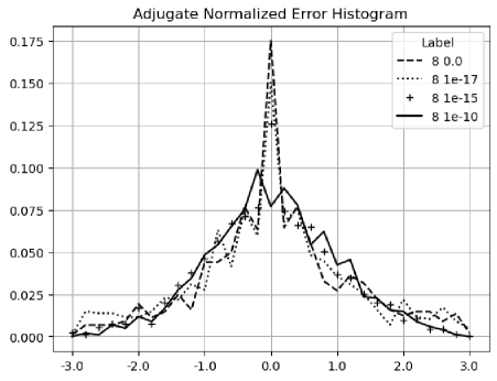
Figure 20 shows that the histograms of the normalized errors is Delta distributed for the input uncertainty $10^{-17}$ , because the adjugate matrix calculation involves about $8\times 6=48$ significand bits for a matrix size $7$ . Such Delta distribution also holds when the matrix size is less than $7$ , or when the input is precise. When the matrix size is $8$ , $8\times 7=56$ significand bits are needed so rounding occurs. As a result, in Figure 21, the distribution becomes Gaussian with a hint of Delta distribution. Such delta-like distribution persists until the input noise precision reaches $10^{-10}$ , which is also the transition of the two trends in Figure 16.

When the input noise precision increases from $10^{-17}$ to $10^{-10}$ , the distributions become less delta-like and more Gaussian, as shown in both Figure 20 and Figure 21. The non-ideal behaviors in Figure 17, 18, and 19 are all attributed to the rounding errors. Table 2 shows that variance arithmetic achieves proper coverage for the calculation rounding errors for adjugate matrix.

Figure 21 suggests that the histogram of normalized errors is more sensitive to rounding errors than the corresponding error deviation, due to averaging effect of the latter. Histograms of normalized errors can be used as a finger-print for the associated calculation. In case error deviation is not known, a nearly Normal-distributed histogram may be used to identify ideal coverage.

6.4 Matrix Inversion

A major usage of $|\mathbf{M}|$ and $\mathbf{M}^{A}$ is to define $\mathbf{M}^{-1}$ in Formula (6.17) which satisfies Formula (6.18). Formula (6.19) gives the Taylor expansion for the element $\mathbf{M}^{-1}_{j,i}$ . From it, $\overline{\mathbf{M}^{-1}_{j,i}}$ and $\delta^{2}\mathbf{M}^{-1}_{j,i}$ can be deduced, in the same way as how Formula (2.6) and (2.3) are deducted from Formula (2.5). Although the analytic expression for $\overline{|\mathbf{M}|}$ and $\delta^{2}|\mathbf{M}|$ is very complex on paper, the deduction is straight-forward in analytic programming such as using SymPy ¹⁰¹⁰10The result of using SymPy for matrix inversion is demonstrated as part of an open source project at https://github.com/Chengpu0707/VarianceArithmetic..

$\displaystyle\mathbf{M}^{-1}$	$\displaystyle\equiv\mathbf{M}^{A}/\|\mathbf{M}\|;$	(6.17)
$\displaystyle(\mathbf{M}^{-1})^{-1}$	$\displaystyle=\mathbf{M};$	(6.18)
$\displaystyle\widetilde{\mathbf{M}^{-1}}_{j,i}$	$\displaystyle=(-1)^{i+j}\frac{\|\widetilde{\mathbf{M}_{i,j}}\|}{\|\widetilde{\mathbf{M}}\|}$	(6.19)
	$\displaystyle=(-1)^{i+j}\left(\sum_{m=0}^{n}\sum_{<i_{1}\dots i_{m}>_{n}}^{i\in\{i_{1}\dots i_{m}\}}\sum_{[j_{1}\dots j_{m}]_{n}}^{j_{i}=j}M_{<i_{1}\dots i_{m}>_{n},[j_{1}\dots j_{m}]_{n}}\prod_{k=1\dots m}^{k\in\{i_{1}\dots i_{m}\}}\tilde{x}_{k,p_{k}}\right)$
	$\displaystyle\;\;\;\sum_{h=0}^{\infty}\frac{(-1)^{h}}{\|M\|^{h+1}}\left(\sum_{m=1}^{n}\sum_{<i_{1}\dots i_{m}>_{n}}\sum_{[j_{1}\dots j_{m}]_{n}}M_{<i_{1}\dots i_{m}>_{n},[j_{1}\dots j_{m}]_{n}}\prod_{k=1\dots m}^{k\in\{i_{1}\dots i_{m}\}}\tilde{x}_{k,p_{k}}\right)^{h};$

Formula (6.19) suggests that $\overline{\mathbf{M}^{-1}}\neq\overline{\mathbf{M}^{A}}/|\mathbf{M}|$ , and $\delta^{2}\mathbf{M}^{-1}$ is much larger than $\delta^{2}\mathbf{M}$ , which agrees with the common practice to avoid using Formula (6.17) directly [13].

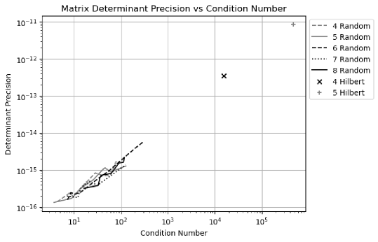
Traditionally, the error response of $\mathbf{M}^{-1}$ is quantified by matrix condition number [37]. In Formula (6.17), $\mathbf{M}^{-1}$ is dominated by $1/|\mathbf{M}|$ , suggesting that the precision of $\mathbf{M}^{-1}$ is largely determined by the precision of $|\mathbf{M}|$ . Variance arithmetic treats the $LSV$ to be imprecise, so it can use Formula (6.14) to calculate the determinant variance for a matrix containing floating-point elements, including a randomly generated matrix, or a Hilbert matrix [37] after it is converted to a floating-point matrix ¹¹¹¹11Although Hilbert matrix is defined using fractional number, its condition number is also calculated using floating-point arithmetic in math libraries such as SciPy.. Figure 22 shows that there is a strong linear correlation between the conditional number and the determinant precision of matrices, so that the determinant precision can replace the condition number, which is more difficult to calculate ¹²¹²12There are currently different definitions of matrix condition number, each based on a different definition of matrix norm..

In fact, condition number may not be the best tool to describe the error response of a matrix. Formula (6.20) shows an example matrix inversion using variance arithmetic representation. It clearly shows the overall precision dominance by the value of $2\pm 0.161$ on the denominator, e.g., $1\pm 0.1$ in the adjugate matrix becomes $-0.510\pm 0.180$ in the inverted matrix, while the direct calculation of $1\pm 0.1/-2\pm 0.161=-0.503\pm 0.065$ has $3$ -fold better result precision. In Formula (6.20), even though the input matrix has element precision ranging from $10^{-1}$ to $2.5\;10^{-5}$ , the inverted matrix has element precision all near $0.2$ except the worst one at $0.35$ , showing how dramatically the element precision gets worse in matrix inversion. Formula (6.19) suggests that the precision of inverted matrix deteriorates exponentially with matrix size.

	$\displaystyle\left(\begin{matrix}1\pm 10^{-1},&2\pm 10^{-2}\\ 3\pm 10^{-3},&4\pm 10^{-4}\end{matrix}\right)^{-1}$	$\displaystyle=\frac{\left(\begin{matrix}4\pm 10^{-4},&-2\pm 10^{-2}\\ -3\pm 10^{-3},&1\pm 10^{-1}\end{matrix}\right)}{-2\pm 0.161}$		(6.20)
		$\displaystyle\simeq\left(\begin{matrix}-2.000\pm 0.401,&1.000\pm 0.201\\ 1.500\pm 0.301,&-0.510\pm 0.180\end{matrix}\right);$

6.5 First Order Approximation

Formula (6.21) shows the first order approximation of $|\widetilde{\mathbf{M}}|$ leads to the first order approximation of $\delta^{2}|\mathbf{M}|$ . It states that when the input precision is much less than $1$ , the determinant $|\mathbf{M}|$ of an imprecise matrix $\mathbf{M}$ can be calculated in variance arithmetic using Formula (6.1) directly.

|\widetilde{\mathbf{M}}|\simeq\sum_{[p_{1}\dots p_{n}]_{n}}\$[p_{1}\dots p_{n}]_{n}\prod_{k=1\dots n}(x_{k,p_{k}}+\tilde{x}_{k,p_{k}});\;\;\;\Rightarrow\;\;\;\delta^{2}|\mathbf{M}|\simeq\sum_{i}^{n}\sum_{j}^{n}M_{i,j}(\delta x_{i,j})^{2};

(6.21)

Figure 23 contains the result of applying Formula (6.21). It is very similar to Figure 17, validating Formula (6.21).

7 Moving-Window Linear Regression

7.1 Moving-Window Linear Regression Algorithm [1]

Formula (7.1) and (7.2) give the result of the least-square line-fit of $Y=\alpha+\beta X$ between two set of data ${Y_{j}}$ and ${X_{j}}$ , in which $j$ is an integer index to identify $(X,Y)$ pairs in the sets [13].

	$\displaystyle\alpha$	$\displaystyle=\frac{\sum_{j}Y_{j}}{\sum_{j}1};$		(7.1)
	$\displaystyle\beta$	$\displaystyle=\frac{\sum_{j}X_{j}Y_{j}\;\sum_{j}1-\sum_{j}X_{j}\;\sum_{j}Y_{j}}{\sum_{j}X_{j}X_{j}\;\sum_{j}1-\sum_{j}X_{j}\;\sum_{j}X_{j}};$		(7.2)

In many applications, data set ${Y_{j}}$ is an input data stream collected with fixed rate in time, such as a data stream collected by an ADC (Analogue-to-Digital Converter) [38]. ${Y_{j}}$ is called a time-series input, in which $j$ indicates time. A moving window algorithm [13] is performed in a small time-window around each $j$ . For each window of calculation, ${X_{j}}$ can be chosen to be integers in the range of $[-H,+H]$ in which $H$ is an integer constant specifying window’s half width so that $\sum_{j}X_{j}=0$ , to reduce Formula (7.1) and (7.2) into Formula (7.3) and (7.4), respectively [1]:

	$\displaystyle\alpha_{j}$	$\displaystyle=\alpha\;2H=\sum_{X=-H+1}^{H}Y_{j-H+X};$		(7.3)
	$\displaystyle\beta_{j}$	$\displaystyle=\beta\;\frac{H(H+1)(2H+1)}{3}=\sum_{X=-H}^{H}XY_{j-H+X};$		(7.4)

The calculation of $(\alpha_{j},\beta_{j})$ can be obtained from the previous values of $(\alpha_{j-1},\beta_{j-1})$ , to reduce the calculation of Formula (7.3) and (7.4) into a progressive moving-window calculation of Formula (7.5) and (7.6), respectively [1]

	$\displaystyle\beta_{j}$	$\displaystyle=\beta_{j-1}-\alpha_{j-1}+H\left(Y_{j-2H-1}+Y_{j}\right);$		(7.5)
	$\displaystyle\alpha_{j}$	$\displaystyle=\alpha_{j-1}-Y_{j-2H-1}+Y_{j};$		(7.6)

7.2 Variance Adjustment

When the time series contains uncertainty, the direct application of Formula (7.5) and (7.6) will result in loss of precision, because both formulas use each input multiple times and accumulate the variance of the input once at each usage. Thus, the values for $\alpha_{j}$ and $\beta_{j}$ should be calculated progressively using Formula (7.6) and (7.5), while the variance should be calculated using Formula (7.7) and (7.8), respectively. Formula (7.8) is no longer progressive.

	$\displaystyle\delta^{2}\alpha_{j}$	$\displaystyle=\sum_{X=-H+1}^{H}(\delta Y_{j-H+X})^{2}=\delta^{2}\alpha_{j-1}+(\delta Y_{j})^{2}-(\delta Y_{j-2H})^{2};$		(7.7)
	$\displaystyle\delta^{2}\beta_{j}$	$\displaystyle=\sum_{X=-H+1}^{H}X^{2}(\delta Y_{j-H+X})^{2};$		(7.8)

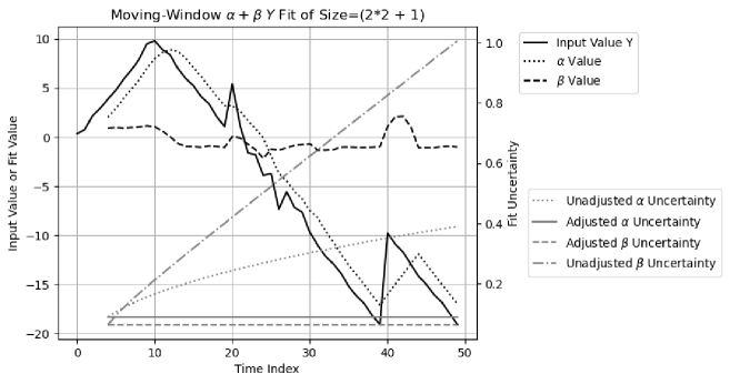
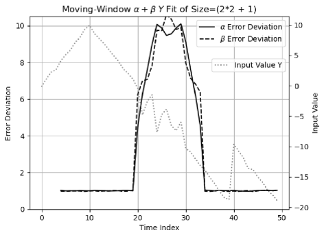
Figure 24 shows that the input signal $Y_{j}$ is composed of:

1.

An increasing slope for $j=0\dots 9$ .
2.

A decreasing slope for $j=1\dots 39$ .
3.

A sudden jump with an intensity of $+10$ at $j=40$
4.

A decreasing slope for $j=41\dots 49$ .

For each increase of $j$ , the increasing rate and the decreasing rate are $+1$ and $-1$ , respectively.

The specified input uncertainty is always $0.2$ . Normal noises of $0.2$ deviation are added to the slopes, except Normal noises of $2$ deviation are added to the slope for $j=10\dots 19$ , during which the actual noises are $10$ -fold of the specified value.

Figure 24 also shows the result of moving window fitting of $\alpha+\beta\;Y$ vs time index $j$ . The result values of $\alpha$ and $\beta$ behave correctly with the expected delay in $j$ . When Formula (7.3) and (7.4) are used both for values and uncertainties for $\alpha$ and $\beta$ , the result uncertainties of $\alpha$ and $\beta$ both increase exponentially with the index time $j$ . When Formula (7.3) and (7.4) are used only for values, while Formula (7.7) and (7.8) are used for variance for $\alpha$ and $\beta$ , the result uncertainty of $\alpha$ is $\sqrt{\frac{1}{2H+1}}\delta Y$ , and the result uncertainty of $\beta$ is $\sqrt{\frac{3}{H(H+1)(2H+1)}}\delta Y$ , both of which are less than the input uncertainty $\delta Y$ , due to the averaging effect of the moving window.

7.3 Unspecified Input Error

To obtain the error deviation of $\alpha$ and $\beta$ , the fitting is done on many time-series data, each with independent generated noises. Figure 25 shows the corresponding error deviation vs index time $j$ , which are $1$ except near $10$ for $j=10\dots 19$ when the actual noise is $10$ -fold of the specified one. It shows that a larger than $1$ error deviation may probably indicate unspecified additional input errors other than rounding errors, such as the numerical errors from math libraries.

8 Fast Fourier Transformation

8.1 Discrete Fourier Transformation (DFT)

For each signal sequence $h[k],k=0,1\dots N-1$ , in which $N$ is a positive integer, the discrete Fourier transformation $H[n],n=0,1\dots N-1$ and its reverse transformation is given by Formula (8.1) and (8.2), respectively [13], in which $k$ is the index time and $n$ is the index frequency for the discrete Fourier transformation (DFT) ¹³¹³13The index frequency and index time are not necessarily related to time unit. The naming is just a convenient way to distinguish the two opposite domains in the Fourier transformation: the waveform domain vs the frequency domain..

		$\displaystyle H[n]=\sum_{k=0}^{N-1}h[k]\;e^{i2\pi kn/N};$		(8.1)
		$\displaystyle h[k]=\frac{1}{N}\sum_{n=0}^{N-1}H[n]\;e^{-i2\pi nk/N};$		(8.2)

8.2 FFT (Fast Fourier Transformation)

When $N=2^{L}$ , in which $L$ is a positive integer, the generalized Danielson-Lanczos lemma [13] can be applied to the discrete Fourier transformation as FFT [13].

•

For each output, each input is only used once, so there is no dependency problem when using Formula (2.11), (2.12), (2.13), and (2.14) as arithmetic operations.
•

When $L$ is large, the large amount of input and output data enables high quality statistical analysis.
•

The amount of calculation is $L$ , because for each output, increasing $L$ by 1 results in one additional step of sum of multiplication.
•

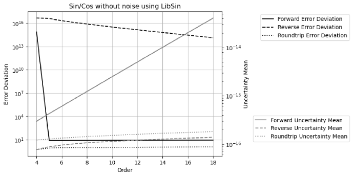
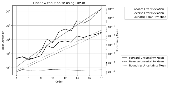
Each step in the forward transformation thus increases the variance by $2$ -fold, so that the result uncertainty mean increases with the FFT order $L$ as $\sqrt{2}^{L}$ . Because the reverse transformation divides the result by $2^{L}$ , the result uncertainty mean decreases with the FFT order $L$ as $\sqrt{1/2}^{L}$ . The result uncertainty mean for the roundtrip transformations is thus $\sqrt{2}^{L}\times\sqrt{1/2}^{L}=1$ .
•

Forward and reverse transformations are identical except for a sign, so they are essentially the same algorithm, and their difference is purely due to input data.

Forward and reverse FFT transforms have data difference in normal usage:

•

The forward transformation cancels real imprecise data of a Sin/Cos signal into a spectrum of mostly $0$ values, so that both its value errors and its result uncertainties are expected to grow faster.
•

The reverse transformation spread the spectrum of precise values of most $0$ to data of a Sin/Cos signal, so that both its value errors and its result uncertainties are expected to grow slower.

8.3 Testing Signals

To avoid unfaithfulness of discrete Fourier transformation to continuous transformation [1], only Formula (8.1) and (8.2) with integer $n$ and $k$ will be used.

The following signals are used for testing:

•

Sin: $h[k]=\sin(2\pi kf/N),f=1,2,...N/2-1$ .
•

Cos: $h[k]=\cos(2\pi kf/N),f=1,2,...N/2-1$ .

•

Linear: $h[k]=k$ , whose discrete Fourier transformation is Formula (8.3).

		$\displaystyle y\equiv i2\pi\frac{n}{N}:\;\;\;G(y)=\sum_{k=0}^{N-1}e^{yk}=\frac{e^{Ny}-1}{e^{y}-1}=\begin{cases}y=0:\;\;\;N\\ y\neq 0:\;\;\;0\end{cases};$
	$\displaystyle H[n]$	$\displaystyle=\frac{dG}{dy}=\begin{cases}n=0:\;\;\;\frac{N(N-1)}{2}\\ n\neq 0:\;\;\;-\frac{N}{2}(1+i/\tan(n\frac{\pi}{N}))\end{cases};$		(8.3)

Empirically:

•

The results from Sin and Cos signals are statistically indistinguishable from each other.
•

The results from Sin signals at different frequencies are statistically indistinguishable from each other.

Thus, the results for Sin and Cos signals at all frequencies are pooled together for the statistical analysis, as the Sin/Cos signals.

8.4 Library Errors

Formula (8.1) and (8.2) limit the use of $\sin(x)$ and $\cos(x)$ to $x=2\pi j/N$ . To minimize the numerical errors of $\sin(x)$ and $\cos(x)$ , indexed sine functions can be used instead of the library sine functions ¹⁴¹⁴14The $\sin$ and $\cos$ library functions in Python, C++, Java all behave in the same way. The indexed sine functions are similar to $sinpi$ and $cospi$ functions proposed in C++23 standard but not readily available excepted in few selected platforms such as for Apple.

1.

Instead of a floating-point value $x$ for $\sin(x)$ and $\cos(x)$ , the integer $j$ is used to specify the input to $\sin(x)$ and $\cos(x)$ , as $\sin(2\pi j/N)$ and $\cos(2\pi j/N)$ , to avoid the floating-point rounding error of $x$ .
2.

The values of $\sin(2\pi j/N)$ and $\cos(2\pi j/N)$ are extended from $j=0,1,\dots N/8$ to $j=0,1,\dots N$ using the symmetry of $\sin(2\pi j/N)$ and $\cos(2\pi j/N)$ .
3.

The values of $\sin(2\pi j/N)$ and $\cos(2\pi j/N)$ are extended from $j=0,1,\dots N$ to the whole integer region using the periodicity of $\sin(2\pi j/N)$ and $\cos(2\pi j/N)$ .

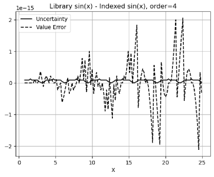
Figure 26 shows that the value difference between the library $\sin(x)$ and the indexed $\sin(x)$ increases with increasing $x$ . However, checked by $\sin(x)^{2}+\cos(x)^{2}-1$ , Figure 27 shows that the value errors are quite comparable between the indexed and library $\sin(x)$ and $\cos(x)$ functions. In Figure 27, the deviations of the value errors for the indexed sine function seem less stable statistically, because the deviations of the index sine function are calculated from much less samples: For the FFT order $N$ , the deviations for the indexed sine function contain $2^{N-3}$ data covering $x\in[0,\pi/4]$ , while the deviations for the library sine function contain $2^{2N-1}$ data covering $x\in[0,\pi 2^{N}]$ . Figure 27 also shows that both $\sin(x)$ functions have proper coverage in variance arithmetic. Thus, the difference is just caused by the rounding of $x$ in $\sin(x)$ and $\cos(x)$ library functions.

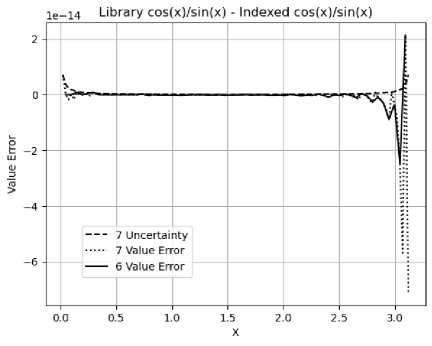
Figure 28 shows the value difference between the library $\cos(x)/\sin(x)$ and the indexed $\cos(x)/\sin(x)$ for $x\in(0,\pi)$ . It covers all the integer inputs to the indexed cotan functions used for the Linear signal of FFT order $6$ and $7$ . The value errors near $x=\pi$ increase with the FFT order. It is likely that the rounding error of $x$ causes the numerical error when $\cos(x)/\sin(x)$ becomes very large near $x=\pi$ . According to Figure 29, the library $\cos(x)/\sin(x)$ function does not have proper coverage in variance arithmetic.

Figure 28 pin-points the deficit of the current $\sin(x)$ and $\tan(x)$ library functions: near $x=n\pi$ . It also indicates the deficit of the current forward rounding error study [12]: near $x=n\pi$ , and without mathematical relation test.

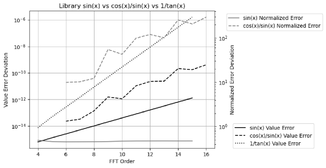
Using indexed $\sin(x)$ as standard, Figure 29 compares the value errors of the library $\sin(x)$ , $\cos(x)/\sin(x)$ , and $1/tan(x)$ for increasing FFT orders. It shows that the numerical errors of all these library functions grow exponentially with increasing FFT order. $1/tan(x)$ has the largest errors, and it will not be used for FFT. $\cos(x)/\sin(x)$ has larger errors than those of $\sin(x)$ .

The difference between the indexed and library sine functions shows the inconsistency in the library sine functions, because the indexed sine functions is just the library sine functions in the range of $[0,\pi/4]$ , and should be related to other ranges according to precise mathematical relations. It is difficult to study the numerical errors of library functions using conventional floating-point arithmetic which has no concept of imprecise values. Having identified the nature and the strength of the numerical errors of the library $\sin(x)$ and $\cos(x)/\sin(x)$ , variance arithmetic can show their effects using FFT.

8.5 Using the Indexed Sine Functions for Sin/Cos Signals

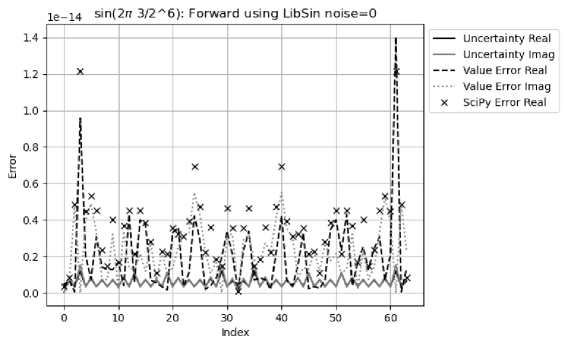
Using the indexed sine functions, for the waveform of $\sin(2\pi j3/2^{6})$ in which $j$ is the index time:

•

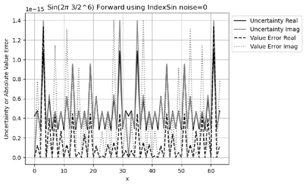
Figure 30 shows that for the forward transformation, the result value errors are comparable to the result uncertainties, with an error deviation of $0.37$ for the real part, and $0.93$ for the imaginary part. Both real and imaginary uncertainties peak at the expected index of $\pm 3$ , but only real value error peak at the frequency. Both real and imaginary uncertainties peak at the unexpected index of $\pm 29$ , $\pm 13$ and $\pm 18$ , as well as the value errors. The reason for the unexpected peaks is not clear. Overall, the uncertainty seems a smoothed version of the value error, and they are comparable in strength.
•

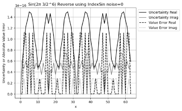
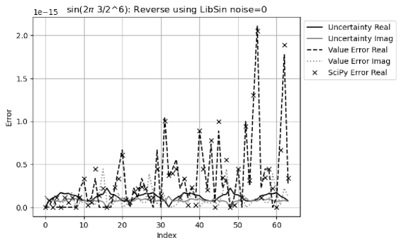
Figure 31 shows that for the reverse transformation, the result value errors are comparable to the result uncertainties, with an error deviation of $0.54$ for the real part, and $0.52$ for the imaginary part. The uncertainty captures the periodicity of the value error, as well as bigger strength of the real value error than that of the imaginary value error.

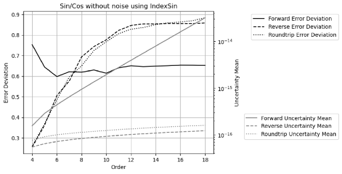
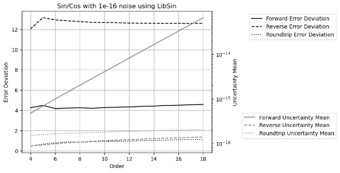
Figure 32 shows both the result uncertainty means and the error deviations vs. FFT order of DTF of Sin/Cos signals using the indexed sine functions. As expected, the uncertainties grow much faster with increasing FFT order for the forward transformation. The error deviations are a constant about $0.65$ for the forward transformation, while they increase with increasing FFT order from $0.25$ until reach a constant about $0.85$ when the FFT order is $12$ or more for the reverse and roundtrip transformation.

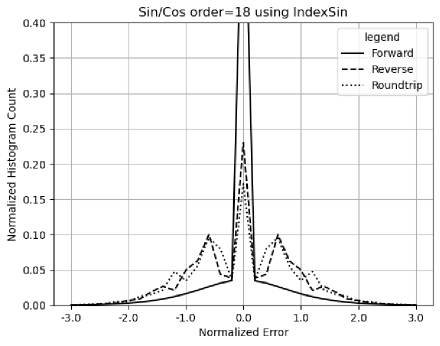
With increasing FFT order, all histograms become more Gaussian like, and the error deviations for the real and the imaginary parts become more equal in value. Figure 33 shows the corresponding histograms of the normalized errors at FFT order $18$ . The distribution of the forward transformation is a larger Delta distribution on top of a Gaussian distribution, while it is a structured distribution on top of a Gaussian distribution for the reverse transformation. The distribution of the roundtrip transformation is almost identical to that of the reverse transformation, suggesting that the presence of input uncertainty for the reverse transformation is not a major factor.

Proper coverage is achieved using the indexed sine functions for Sin/Cos signals.

8.6 Using the Library Sine Functions for Sin/Cos Signals

Because the least significant values are the only source of input uncertainties for variance arithmetic, the result uncertainties using either indexed or library sine functions are almost identical. The library sine functions have numerical calculation errors which are not specified by the input uncertainties of variance arithmetic. The question is whether variance arithmetic can track these numerical errors effectively or not.

Using the library sine functions, for the waveform of $\sin(2\pi j3/2^{6})$ in which $j$ is the index time:

•

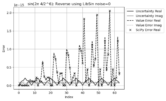
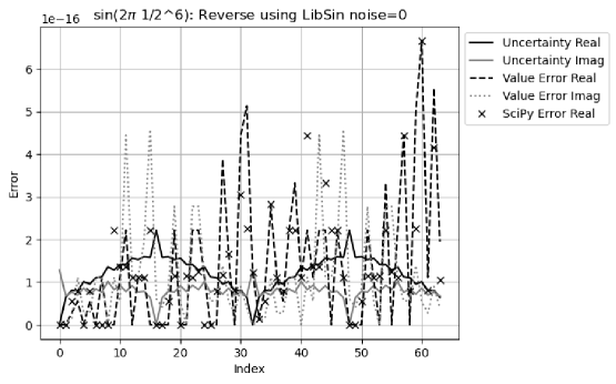
Figure 34 shows that for the forward transformation, the result value errors are noticeably larger than the result uncertainties, with an error deviation of $7.0$ for the real part, and $5.6$ for the imaginary part. As expected, the error deviations are noticeably larger than their counterparts in Figure 30.
•

Figure 35 shows that for the reverse transformation, the result value errors are noticeably larger than the result uncertainties, with an error deviation of $5.7$ for the real part, and $0.83\;10^{15}$ for the imaginary part. The surprisingly large imaginary error deviation is caused by the small uncertainty at the index time of $8$ where the value error is at a local maximum.
•

Because of the result of the huge error deviation, Figure 36 shows that the result of the reverse transformation no longer has proper coverage for all FFT orders. When a small noise with deviation of $10^{-16}$ is added to the input, the result uncertainty of the reverse transformation at the index time of $8$ is no longer near $0$ , so that the result error deviations achieve proper coverage again, as show in Figure 37.
•

Figure 32 and Figure 36 confirm that the result uncertainties are identical to all FFT, respectively.

Variance arithmetic reveals why to add small noises to the numerically generated input data, which is already a common practice [13]. It further reveals that the amount of noise needed is to achieve proper coverage.

In Figure 35, the value errors tend to increase with the index time, which is due to the periodic increase of the numerical errors of $\sin(x)$ with $x$ as shown in Figure 26. When the signal frequency increases, the increase of the value errors with the index frequency in the reverse transformation becomes stronger, as shown in Figure 35, 38, and 39. In fact, Figure 38 suggests that the periodic numerical errors in Figure 26 resonate with the periodicity of the input $Sin$ signal. In contrast, Figure 31 shows no sign for such increase. It shows that the library numerical errors may have surprisingly large effect on the numerical results.

To validate the FFT implementation in variance arithmetic, the results are compared with the corresponding calculations using the python numerical library SciPy in Figure 34 and 35. The results are quite comparable, except that in SciPy, the data waveform is always real rather than complex. In Figure 34, the SciPy results have been made identical for the frequency indexes $f$ and $-f$ , and the matching to the corresponding results of variance arithmetic is moderate. In Figure 35, the SciPy results match the corresponding results of variance arithmetic quite well. It shows that the effects of library numerical errors revealed by variance arithmetic exist in real applications.

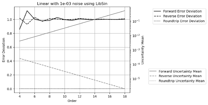
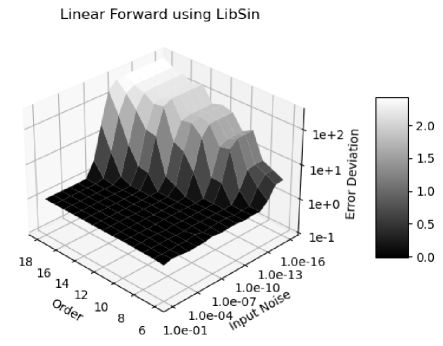
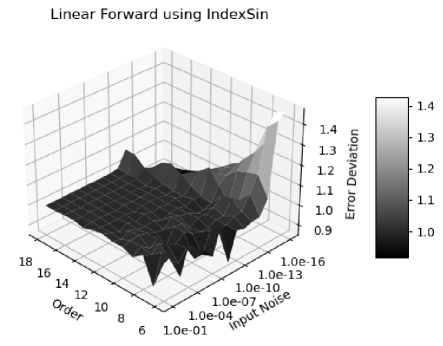
8.7 Linear Signal

As shown in Figure 29, linear signals may introduce more numerical errors to the result through library $\cos(x)/sin(x)$ . The question is whether variance arithmetic can track these additional numerical errors or not.

Using the indexed sine functions:

•

Figure 40 shows that the result uncertainty for each FFT transformation has much larger increase with the increasing FFT order than its counterpart in Figure 32. The much faster uncertainty increase of the forward transformation is attributed to the non-zero input uncertainties. Figure 40 shows that proper coverage can be achieved for all FFT for all FFT orders.
•

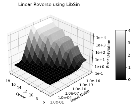
Figure 41 shows that for each transformation, the histogram of the Linear signal is somewhat similar to the counterpart of the Sin/Cos signals in Figure 33, except that the histograms for linear signal have larger Gaussian background.

Using the library sine functions:

•

Figure 42 shows that proper coverage cannot be achieved for all FFT for all FFT orders, because the value errors outpace the uncertainties with increasing FFT order, to result in worse error deviations for increasing FFT order.
•

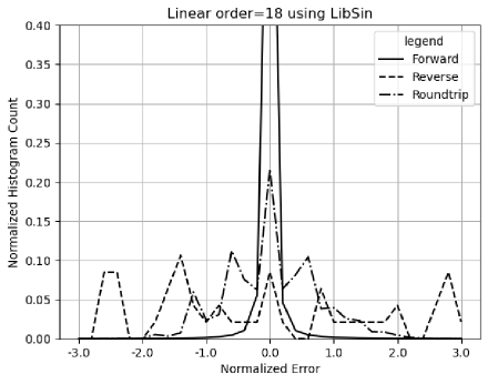
Figure 43 shows that the reverse histogram contains additional peaks to its counterpart in Figure 41. The additional peaks extend quite beyond the range of $[-3,+3]$ , revealing why variance arithmetic cannot cover these value errors. Such large numerical errors are expected from Figure 29.

The result difference using variance arithmetic for library Sin/Cos signal vs library Linear signal suggests that variance arithmetic can break down when the input contains too much unspecified errors. The only solution seems to create a new sin library using variance arithmetic so that all numerical calculation errors are accounted for.

8.8 Ideal Coverage

Adding enough noise to the input can overpower unspecified input errors, to achieve ideal coverage, such as $10^{-3}$ input noise for Linear signal using the library sine functions.

•

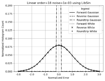
Figure 44 shows the corresponding histogram. As expected, the normalized errors for the forward and the reverse transformations are Normal distributed. The normalized errors for the roundtrip transformations are Delta distributed at $0$ , meaning the input uncertainties are perfectly recovered.
•
Figure 45 show the corresponding error deviations and uncertainty means:
- –
  
  As expected, the result uncertainty means for the forward transformations increase with the FFT order $L$ as $\sqrt{2}^{L}$ .
- –
  
  As expected, the result uncertainty means for the reverse transformations decrease with the FFT order $L$ as $\sqrt{1/2}^{L}$ .
- –
  
  As expected, the result uncertainty means for the roundtrip transformations always equal the corresponding input uncertainties of $10^{-3}$ .
- –
  
  As expected, the result error deviations for the forward and reverse transformations are constant $1$ , while the result error deviations for the roundtrip transformation approaches $0$ exponentially with increasing FFT order.

Also, the result uncertainty means for both the forward and the reverse transformations are linear to the input uncertainties, respectively, which is expected because FFT is linear.

The range of ideal coverage depends on how well the input uncertainty specifies the input noise. For Linear signals using library sine functions, Figure 46 and 47 show the error deviation vs. the added noise vs. FFT order for the forward and reverse transformations, respectively. The ideal coverage is shown as the regions where the error deviations are $1$ . In other regions, proper coverage is not achievable. Because the uncertainties grow slower in the reverse transformation than in the forward transformation, the reverse transformations have smaller ideal coverage region than that of the forward transformation. Because numerical errors increase with the amount of calculation, the input noise range for ideal coverage reduces with increasing FFT order. It is possible that ideal coverage is not achievable at all, e.g., visually, when the FFT order is larger than $25$ for the reverse transformation. As one of the most robust numerical algorithms that is very insensitive to input errors, FFT can breaks down due to the numerical errors in the library sine functions, and such deterioration of the calculation result is not easily detectable using the conventional floating-point calculation.

In contrast, for Linear signals using indexed sine functions, as shown by Figure 48 and 49 for the forward and reverse transformations, respectively, the ideal region is much larger, and proper coverage is achieved in other regions. Forward FFT transformation shows larger region of ideal coverage than that of Reverse FFT transformation.

As an comparison, because sin/cos has less numerical calculation errors, for Sin/Cos using either indexed sine functions or library sine functions, the ideal region is achieved when the added noise is large enough to cover the effect of rounding errors, almost independent of FFT orders. In both cases, forward transformation needs $10^{-15}$ added noise, while reverse transformation needs $10^{-12}$ added noise. The difference is that using indexed sine functions, in the proper coverage region, error deviations deviate from $1$ only slightly.

8.9 Summary

The library sine functions using conventional floating-point arithmetic have been shown to contain numerical errors as large as equivalently $10^{-3}$ of input precision for FFT. The library $\sin(x)$ errors increase periodically with $x$ , causing noticeable increase of the result errors with increasing index frequency in the reverse transformation, even in resonant fashion. The dependency of the result numerical errors on the amount of calculation and input data means that a small-scale test cannot properly qualify the result of a large-scale calculation. The effect of numerical errors inside math library has not been addressed seriously.

Variance arithmetic should be used, whose values largely reproduce the corresponding results using conventional floating-point arithmetic, whose uncertainties trace all input errors, and whose result error deviations qualify the calculation quality as either ideal, or proper, or suspicious. If the library functions also have proper coverage, the calculation result will probably have proper coverage as well.

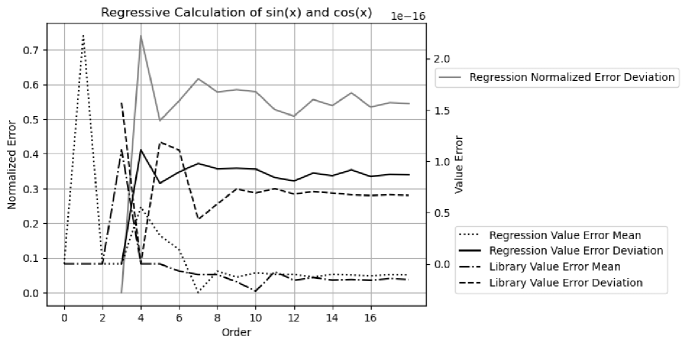
9 Regressive Generation of Sin and Cos

Formula (9.2) and Formula (9.3) calculate $\sin(j\frac{\pi}{2n}),\cos(j\frac{\pi}{2n}),j=0\dots N$ repressively starting from Formula (9.1), .

$\displaystyle\sin(0)=\cos(\frac{\pi}{2})=0;$	$\displaystyle\sin(\frac{\pi}{2})=\cos(0)=1;$	(9.1)
$\displaystyle\sin\left(\frac{\alpha+\beta}{2}\right)=\sqrt{\frac{1-\cos\left(\alpha+\beta\right)}{2}}=$	$\displaystyle\sqrt{\frac{1-\cos(\alpha)\cos\left(\beta)+\sin(\alpha\right)\sin(\beta)}{2}};$	(9.2)
$\displaystyle\cos\left(\frac{\alpha+\beta}{2}\right)=\sqrt{\frac{1+\cos\left(\alpha+\beta\right)}{2}}=$	$\displaystyle\sqrt{\frac{1+\cos(\alpha)\cos(\beta)-\sin(\alpha)\sin(\beta)}{2}};$	(9.3)

When $\alpha+\beta\rightarrow 0$ , the nominator in Formula (9.2) is the difference of two values both are very close to $1$ , to result in very coarse precision. Also, both value errors and uncertainties are accumulated in the regression. This regression is not suitable for calculating library $\sin$ and $\cos$ functions. It can be used to check the trigonometric relation for library $\sin$ and $\cos$ functions.

The number of regressions is defined as the order. For each order $n$ , $2^{n}$ $\sin(j\frac{\pi}{2n})$ and $\cos(j\frac{\pi}{2n})$ values are obtained, so that the result is more statistically stable with increasing $n$ .

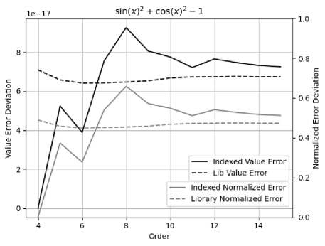
The value errors of $\sin(x)$ and $\cos(x)$ are checked by $\sin(x)^{2}+\cos(x)^{2}-1$ . Figure 50 shows that the value errors of the generated $\sin(x)$ and $\cos(x)$ is comparable to those of library $\sin(x)$ and $\cos(x)$ . It shows that the result error deviations are close to $0.5$ . Because floating-point rounding errors are the only source of errors in the regression, as expected, variance arithmetic provides proper coverage for this regression.

10 Conclusion and Discussion

10.1 Summary of Statistical Taylor Expansion

The starting point of statistical Taylor expansion is the uncorrelated uncertainty assumption of all input variables. It is a very reasonable statistical requirement on the input data [1]. Once the uncorrelated uncertainty assumption is satisfied, statistical Taylor expansion quantifies uncertainty as the deviation of the value errors. It can trace the variable dependency in the intermediate steps using standard statistics. It no longer has dependency problem, but demands a much more rigid process to obtain the result mean and deviation of an analytic expression.

Statistical Taylor Expansion suggests that a calculation result such as its convergence depends on input bounding factors, which may be another measurement of data quality.

10.2 Summary of Variance Arithmetic

Variance arithmetic simplifies statistical Taylor expansion by assuming that all input are Gaussian distributed. The statistical nature of variance arithmetic is reflected by the bounding leakage $\epsilon=5.73\;10^{-7}$ . Ill-formed problems can invalidate the result as: variance not convergent, value not stable, variance not positive, variance not finite, and variance not reliable.

The presence of ideal coverage is the necessary condition for a numerical algorithm in variance arithmetic to be correct. The ideal coverage also defines the ideal applicable range for the algorithm. In ideal coverage, the calculated uncertainty equals the value error deviation, and the result normalized errors is either Normal distributed or Delta distributed depending on the context. In variance arithmetic, the best-possible precision to achieve ideal coverage is $10^{-15}$ , which is good enough for most applications.

Variance arithmetic can only provide proper coverage for floating-point rounding errors, with the empirical error deviations in the approximate range of $[1/5,5]$ . Table 3 shows the measured error deviations in different contexts.

Variance arithmetic has been showcased to be widely applicable, so as for analytic calculations, progressive calculation, regressive generalization, polynomial expansion, statistical sampling, and transformations.

The code and analysis for variance arithmetic are published as an open source project at https://github.com/Chengpu0707/VarianceArithmetic.

Context	Error Deviation
Adjugate Matrix	$4$
$\sqrt[p]{x^{p}}-x$	$0.55$
Forward FFT of Sin/Cos signal with indexed sine	$0.65$
Reverse FFT of Sin/Cos signal with indexed sine	$0.85$
Roundtrip FFT of Sin/Cos signal with indexed sine	$0.87$
Forward FFT of Linear signal with indexed sine	$0.8$
Reverse FFT of Linear signal with indexed sine	$1.0$
Roundtrip FFT of Linear signal with indexed sine	$1.25$
Regressive Calculation of sin and cos	$0.55$

Table 3: The error deviations for floating-point rounding errors in different contexts.

10.3 Improvement Needed

This paper just showcases variance arithmetic which is still in its infancy. Theoretically, some important questions remain:

•

Is there a way for variance arithmetic to provide ideal coverage to floating-point rounding errors? Many theoretical calculations have no input uncertainties, so that when the generation mechanism for rounding error is thoroughly understood, a special version of variance arithmetic for ideal coverage to floating-point rounding errors may be desirable.
•

What is the uncertainty upper bounds for each problem? Specifically, how to explain quantitatively the measured upper bounds in Figure 3 for $(x+\delta x)^{c}$ , and Figure 4 for $\sin(x+\delta x)$ ?
•

How to apply variance arithmetic when analytic solution is not available such as solving differential equation?
•

How to extend variance arithmetic to other input uncertainty distribution?

Traditional numerical approaches focus primarily on the result values, and they need to be reexamined or even reinvented in variance arithmetic. Most traditional numerical algorithms try to choose one of the best paths, while variance arithmetic rejects conceptually all path-dependent calculations. How to reconcile variance arithmetic and traditional numerical approaches could be a big challenge.

The calculation of the result mean and uncertainty contains a lot of sums of constant terms such as Formula (2.3) and (2.3), so that it is a excellent candidate for parallel processing. Because variance arithmetic has neither execution freedoms nor the associated dependency problems, it can be implemented either in software using GPU or directly in hardware.

In variance arithmetic, it is generally an order-of-magnitude more complicated to calculate the result uncertainties than the result values, such as Formula (6.19) for Taylor expansion of matrix inversion. However, modern software programs for analytic calculation such as SymPy can be a great help. Perhaps it is time to move from numerical programming to analytic programming for analytic problems.

10.4 Recalculating Library Math Functions

The library math functions need to be calculated using variance arithmetic, so that each output value has its corresponding uncertainty. Otherwise, the effect of the existing value errors in the library function can have unpredictable and large effects. For example, this paper shows that the periodic numerical errors in the sine library functions cause resonant-like large result value errors in a FFT reverse transformation.

10.5 Different Floating-Point Representation for Variance

In variance representation $x\pm\delta x$ , $\delta x$ is comparable in value with $x$ , but $(\delta x)^{2}$ is calculated and stored. This limits the effective range for $x\pm\delta x$ to be much smaller than the full range of the standard 64-bit floating-point representation. Ideally, $(\delta x)^{2}$ should be calculated and stored in an unsigned 64-bit floating-point representation in which the sign bit reused for the exponent, so that $\delta x$ has exactly the same range as the standard 64-bit floating-point representation.

10.6 Lower Order Approximation

Most practical calculations are neither pure analytic nor pure numerical, in which the analytic knowledge guides the numerical approaches, such as solving differential equations. In these cases, when input precision is fine enough, lower-order approximation of variance arithmetic may be a viable solution because these calculations may only have low-order derivatives for the result. This paper provides an example of first order approximation of variance arithmetic, as Formula (6.21) for $\delta^{2}|\mathbf{M}|$ . According to Section 3, the convergence and stability of the result has to be assumed for lower-order approximations. How to effectively apply variance arithmetic to practical calculations remains an open question.

10.7 Source Tracing

As an enhancement for dependency tracing, source tracing points out the contribution to the result uncertainty bias and uncertainty from each input. This gives clues to engineers on how to improve a measurement effectively.

10.8 Variable $\sigma$ Variance Arithmetic

Variance arithmetic rejects a calculation if its distributional pole or distributional zero is within the input ranges. But there are many use cases in which such intrusion cannot be avoided, so variance arithmetic of smaller $\sigma$ may be needed. It is even possible in another implementation of statistical Taylor expansion, $\sigma$ is part of a variance representation, so that a calculation closer to a distributional zero can proceed but at the expense of reducing $\sigma$ . The result $\sigma$ for a calculation of imprecise inputs each with different $\sigma$ is found statistically through the corresponding $\epsilon$ . Such approaches need theoretical foundation in both mathematics and statistics.

10.9 Acknowledgments

As an independent researcher without any academic association, the author of this paper feels indebted to encouragements and valuable discussions with Dr. Zhong Zhong from Brookhaven National Laboratory, Prof Weigang Qiu from Hunter College, the organizers of AMCS 2005, with Prof. Hamid R. Arabnia from University of Georgia in particular, and the organizers of NKS Mathematica Forum 2007, with Dr. Stephen Wolfram in particular. Prof Dongfeng Wu from Louisville University provides valuable guidance and discussions on statistical related topics. The author of this paper is very grateful for the editors and reviewers of Reliable Computing for their tremendous help in shaping and accepting the previous version of this paper from unusual source, with managing editor, Prof. Rolph Baker Kearfott in particular.

References

[1] C. P. Wang. A new uncertainty-bearing floating-point arithmetic. Reliable Computing, 16:308–361, 2012.
[2] Sylvain Ehrenfeld and Sebastian B. Littauer. Introduction to Statistical Methods. McGraw-Hill, 1965.
[3] John R. Taylor. Introduction to Error Analysis: The Study of Output Precisions in Physical Measurements. University Science Books, 1997.
[4] Jurgen Bortfeldt, editor. Fundamental Constants in Physics and Chemistry. Springer, 1992.
[5] Michael J. Evans and Jeffrey S. Rosenthal. Probability and Statistics: The Science of Uncertainty. W. H. Freeman, 2003.
[6] Fredrik Gustafsson and Gustaf Hendeby. Some relations between extended and unscented kalman filters. IEEE Transactions on Signal Processing, 60-2:545–555, 2012.
[7] John P Hayes. Computer Architecture. McGraw-Hill, 1988.
[8] David Goldberg. What every computer scientist should know about floating-point arithmetic. ACM Computing Surveys, March 1991.
[9] Institute of Electrical and Electronics Engineers. ANSI/IEEE 754-2008 Standard for Binary Floating-Point Arithmetic, 2008.
[10] U. Kulish and W.M. Miranker. The arithmetic of digital computers: A new approach. SIAM Rev., 28(1), 1986.
[11] J. H. Wilkinson. Rounding Errors in Algebraic Processes. SIAM, 1961.
[12] Nicholas J. Higham. Accuracy and Stability of Numerical Algorithms. SIAM, 2002.
[13] William H. Press, Saul A Teukolsky, William T. Vetterling, and Brian P. Flannery. Numerical Recipes in C. Cambridge University Press, 1992.
[14] Oliver Aberth. Precise Numerical Methods Using C++. Academic Press, 1998.
[15] Nicholas J. Higham† and Theo Mary. A new approach to probabilistic rounding error analysis. SIAM Journal on Scientific Computing, 41(5):A2815–A2835, 2019.
[16] B. Liu and T. Kaneko. Error analysis of digital filters realized with floating-point arithmetic. Proc. IEEE, 57:p1735–1747, 1969.
[17] B. D. Rao. Floating-point arithmetic and digital filters. IEEE, Transations on Signal Processing, 40:85–95, 1992.
[18] Gregory L. Baker and Jerry P. Gollub. Chaotic Dynamics: An Introduction. Cambridge University Press, 1990.
[19] Brian Gladman, Vincenzo Innocente, John Mather, and Paul Zimmermann. Accuracy of mathematical functions in single, double, double extended, and quadruple precision. 2024.
[20] R.E. Moore. Interval Analysis. Prentice Hall, 1966.
[21] W. Kramer. A prior worst case error bounds for floating-point computations. IEEE Trans. Computers, 47:750–756, 1998.
[22] G. Alefeld and G. Mayer. Interval analysis: Theory and applications. Journal of Computational and Applied Mathematics, 121:421–464, 2000.
[23] W. Kramer. Generalized intervals and the dependency problem. Proceedings in Applied Mathematics and Mechanics, 6:685–686, 2006.
[24] A. Neumaier S.M. Rump S.P. Shary B. Kearfott, M. T. Nakao and P. Van Hentenryck. Standardized notation in interval analysis. Computational Technologies, 15:7–13, 2010.
[25] W. T. Tucker and S. Ferson. Probability bounds analysis in environmental risk assessments. Applied Biomathmetics, 100 North Country Road, Setauket, New York 11733, 2003.
[26] J. Stolfi and L. H. de Figueiredo. An introduction to affine arithmetic. TEMA Tend. Mat. Apl. Comput., 4:297–312, 2003.
[27] R. Alt and J.-L. Lamotte. Some experiments on the evaluation of functional ranges using a random interval arithmetic. Mathematics and Computers in Simulation, 56:17–34, 2001.
[28] J. Stolfi and L. H. de Figueiredo. Self-validated numerical methods and applications. ftp:// ftp.tecgraf.puc-rio.br/pub/lhf/doc/cbm97.ps.gz, 1997.
[29] Propagation of uncertainty. http://en.wikipedia.org/wiki/Propagation_of_uncertainty, 2011. wikipedia, the free encyclopedia.
[30] S. Ferson H. M. Regan and D. Berleant. Equivalence of methods for uncertainty propagation of real-valued random variables. International Journal of Approximate Reasoning, 36:1–30, 2004.
[31] Significance arithmetic. http://en.wikipedia.org/wiki/Significance_arithmetic, 2011. wikipedia, the free encyclopedia.
[32] M. Goldstein. Significance arithmetic on a digital computer. Communications of the ACM, 6:111–117, 1963.
[33] R. L. Ashenhurst and N. Metropolis. Unnormalized floating-point arithmetic. Journal of the ACM, 6:415–428, 1959.
[34] G. Spaletta M. Sofroniou. Precise numerical computation. The Journal of Logic and Algebraic Programming, 65:113–134, 2005.
[35] J. Vignes. A stochastic arithmetic for reliable scientific computation. Mathematics and Computers in Simulation, 35:233–261, 1993.
[36] C. Denis N. S. Scott, F. Jezequel and J. M. Chesneaux. Numerical ’health’ check for scientific codes: the cadna approach. Computer Physics Communications, 176(8):501–527, 2007.
[37] J. Hefferon. Linear algebra. http://joshua.smcvt.edu/linearalgebra/, 2011.
[38] Paul Horowitz and Hill Winfield. Art of Electronics. Cambridge Univ Press, 1995.

		$\displaystyle\|\mathbf{M}_{<i_{1},i_{2}>_{n},[j_{1},j_{2}]_{n}}\|\equiv\sum_{[p_{1}\dots p_{n}]_{n}}^{p_{i_{1}}=j_{1},p_{i_{2}}=j_{2}}\$[p_{1}\dots p_{n}]_{n}\prod_{k=1\dots n}^{k\not\in\{i_{1},i_{2}\}}x_{k,p_{k}};$		(6.4)
	$\displaystyle\|\mathbf{M}\|$	$\displaystyle=\sum_{j_{1}=1\dots n}x_{i_{1},j_{1}}\|\mathbf{M}_{i_{1},j_{1}}\|=\sum_{j_{1}=1\dots n}\sum_{j_{2}=1\dots n}^{j_{2}\neq j_{1}}\|\mathbf{M}_{<i_{1},i_{2}>_{n},[j_{1},j_{2}]_{n}}\|x_{i_{1},j_{1}}x_{i_{2},j_{2}};$		(6.5)

	$\displaystyle\|\mathbf{M}_{<i_{1}\dots i_{m}>_{n},[j_{1}\dots j_{m}]_{n}}\|\equiv\sum_{[p_{1}\dots p_{n}]_{n}}^{k\in\{i_{1}\dots i_{m}\}:p_{k}=j_{k}}\$[p_{1}\dots p_{n}]_{n}\prod_{k=1\dots n}^{k\not\in\{i_{1}\dots i_{m}\}}x_{k,p_{k}};$	(6.6)
$\displaystyle\|\mathbf{M}\|$	$\displaystyle=\sum_{{[j_{1}\dots j_{m}]}_{n}}\|\mathbf{M}_{<i_{1}\dots i_{m}>_{n},[j_{1}\dots j_{m}]_{n}}\|\prod_{k=1}^{m}x_{i_{k},j_{k}};$	(6.7)
	$\displaystyle\left\|\|\mathbf{M}_{<i_{1}\dots i_{m}>_{n},[j_{1}\dots j_{m}]_{n}}\|\right\|=\left\|\|\mathbf{M}_{<i_{1}\dots i_{m}>_{n},<j_{1}\dots j_{m}>_{n}}\|\right\|;$	(6.8)

Statistical Taylor Expansion111