Statistical Uncertainty Principle in Stochastic Dynamics

The empirical derivation of MaxEnt for state distribution data of independent and identically-distributed (i.i.d.) ensemble has been revisited by one of us [17, 18]. Here, we briefly revisit the data-driven derivation of its extension to correlated data about transitions [12, 13, 14].

Before we begin, let us first remark that applying MaxEnt to stochastic processes is conceptually straightforward from either Jaynes’ argument of least-bias [11] or Shore and Johnson’s axioms [11, 7]: one simply replaces state distribution with path distribution. Jaynes called this the Maximum Caliber principle (MaxCal) [6]. In this generalization, the stochastic process needs not to be Markovian or have a steady state. Once we know the expected values of some path observables, it can be used in MaxCal to provide an update on the our model of path probabilities. However, if one aims to get these expected values from data, one has to rely on the law of large number for convergence, i.e. the data about dynamics has to be either i.i.d. ensembles of paths or the large collections of Markov correlated transitions in a single long path. The former belongs to the formulation of i.i.d. ensembles and has been reviewed before. Here, we focus on the latter generalization where the data is Markov correlated about consequent transitions.

Let us begin by considering (a vector of) transition-based observables $\boldsymbol{g}_{ij}$ in a discrete-time Markov chain (DTMC) where $i$ and $j$ are in the state space $\mathcal{X}$. The steady-state expected value of $\boldsymbol{g}_{ij}$ is

where $\pi_{i}$ is the steady state distribution and $K_{j|i}$ is the underlying transition probability matrix of the DTMC from $i$ to $j$. The ergodic theory for Markov chain tells us that the long-term empirical average of $\boldsymbol{g}_{ij}$ converges to the steady-state mean value $\left\langle\boldsymbol{g}\right\rangle$:

The underlying mechanism of this convergence is the convergence of the joint empirical frequency of a transition pair in a length-$T$ path $x_{0:T}$,

to the steady-state pair probability $\pi_{i}K_{j|i}$ in the long-term limit $T\rightarrow\infty$. These laws of large number for Markov chains are the direct extension from the i.i.d. sample of distribution to correlated-data produced by Markov processes.

Now, similar to the i.i.d. case [19, 18], a key to derive MaxEnt is that the frequency $f_{ij}$ has an asymptotical distribution with an exponential form under a prior Markov chain model with probability $\mathbb{Q}$ [20]:

The matrix $R_{j|i}$ is our prior transition matrix that defines our prior probability $\mathbb{Q}$, and the matrix $f_{j|i}$ is the empirical transition matrix calculated by $f_{ij}/\sum_{k\in\mathcal{X}}f_{ik}$. Then, we can consider three conceptually different posterior joint stationary probability [12], which are all mathematically equivalent in the long-term limit $T\rightarrow\infty:$

a) the asymptotic conditional probability:

where the time label $s$ is a function of $T$, chosen such that $X_{s}$ and $X_{s+1}$ are at the steady state of the process;

b) asymptotic conditional expectation of the empirical pair frequency:

where $\mathbb{E}[\cdot]$ is taken w.r.t. the prior model $\mathbb{Q}$;

c) the most probable empirical frequency:

The three constraints in Eq. (7) are the empirical averages of data ad infinitum, the stationary constraint, and the normalization. The equivalency among the three are known as the Gibbs conditioning principle [21, 12].

We note that the “entropy” to be extremized in the Markov correlated data case here in Eq. (7) is not the Kullback-Leibler relative entropy of pair probabilities $\sum_{i,j\in\mathcal{X}}P_{ij}\ln\frac{P_{ij}}{\pi_{i}^{R}R_{j|i}}$ where $\pi_{i}^{R}$ is the stationary distribution of prior $R_{j|i}$. The fundamental reason of this is because MaxCal is about the whole path $x(t),t>0$, not just one step. This can be seen from the alternative MaxCal derivation of Eq. (7) shown in the Supplemental Material.

Since Eq. (7) is a less-known MaxEnt calculation, we briefly summarize the recipe of computing the posterior joint probability $P_{ij}^{*}$ below. First, we construct a tilted matrix $M_{ij}(\boldsymbol{\beta})=R_{j|i}e^{\boldsymbol{\beta}\cdot\boldsymbol{g}_{i,j}}$. Second, we compute its largest eigenvalue $\lambda$ and the corresponding left and right eigenvectors, $l_{i}$ and $r_{i}$ (chosen such that $\sum_{i\in\mathcal{X}}l_{i}r_{i}=1$). The Perron-Forbenius theorem guarantees that $\lambda$ is real and non-negative $l_{i}$ and $r_{i}$ can be found. Third, the posterior probability transition in terms of $\boldsymbol{\beta}$ is then given by

with the stationary distribution given by $\pi_{i}^{*}=l_{i}(\boldsymbol{\beta})r_{i}(\boldsymbol{\beta})$ and $P_{ij}^{*}=\pi_{i}^{*}P_{j|i}^{*}$. Finally, we solve $\boldsymbol{\beta}$($\left\langle\boldsymbol{g}\right\rangle)$ according to $\left\langle\boldsymbol{g}\right\rangle=\nabla\ln\lambda(\boldsymbol{\beta})$, which is a set of PDEs that can be solved systematically with optimization procedures described later in Eq. (12) and Eq. (13).

Statistical thermodynamics can be derived generally by MaxEnt [7, 18]. And, based on the data-driven empirical derivation of MaxEnt reviewed above, we can consider thermodynamics as emerged from the data infinitus limit, for both i.i.d. ensembles and Markov correlated transitions.

The origin of the thermodynamic structure is the convex duality between a pair of functions, known as entropy and free energy in classical thermodynamics. For i.i.d. data about the distribution of states, the “entropy” is the posterior relative entropy, $\varphi(\left\langle\boldsymbol{g}\right\rangle)\coloneqq\sum_{i\in\Omega}p_{i}^{*}\log\frac{p_{i}^{*}}{q_{i}}$, and the “free energy” is the generating function of the observable $\boldsymbol{g}$, $\psi(\boldsymbol{\beta})\coloneqq\log\sum_{i\in\Omega}e^{\boldsymbol{\beta}\cdot\boldsymbol{g}}$. This is the textbook classical thermodynamics [17, 18]. For transition-based Markov correlated data, the “entropy” becomes the posterior path relative entropy,

and the “free energy” is the scaled generating function for the empirical sum $\boldsymbol{G}_{T}\coloneqq\sum_{t=1}^{T}\boldsymbol{g}_{x_{t-1},x_{t}},$

which becomes the logarithm of the largest eigenvalue $\lambda$ computed by the tilted matrix. In both cases, the “free energy” $\psi$ is a generating function, and the entropy $\varphi$ is the extremized value of a entropy function.

Convex duality between the entropy $\varphi$ and the free energy $\psi$ emerges from limit theorems. On the one hand, the free energy $\psi$ is always the Legendre-Fenchel transform of the entropy $\varphi$.

This is a direct consequence of computing $\psi$ from its definition with the Laplace’s approximation in asymptotic analysis [22, 17]. On the other hand, the inverse of Eq. (11) requires the existence and differentiability of $\psi$. This is known as the Gärtner-Ellis theorem [23, 24, 22]:

These Legendre-Fenchel-transform expressions of $\varphi$ and $\psi$ tell us that both of them are convex functions [22]. With differentiable $\psi$ and $\varphi$, the two Legendre-Fenchel transforms above reduces to a single Legendre transform, which encodes derivative relations between the dual coordinates $\left\langle\boldsymbol{g}\right\rangle$ and $\boldsymbol{\beta}$ of the system,

as well as the Maxwell’s relations associated with them. Importantly, Eq. (13) shows that the parameters $\boldsymbol{\beta}$ are the entropy forces conjugated to the observables $\left\langle\boldsymbol{g}\right\rangle$.

We are now ready to discuss the dynamic extension of the uncertainty principle between the statistical variations of observables (e.g. energy) and of the inferred conjugated entropic forces (e.g. 1/temperature) in thermodynamics [1, 25, 26, 27]. We shall call it the statistical uncertainty principle (SUP) since it is an leading-order statistical result for large but finite data. Our contributions here are twofold: a) We extends SUP from state observables [1, 25, 26] to transition observables, from distribution to dynamics; b) SUP shows the physical meaning of a well-known mathematical relation in large deviation theory.

To illustrate, let’s consider the following scenario. Suppose Bob has transition-based data in the form of the empirical mean $\bar{\boldsymbol{g}}_{T}=\sum_{i,j\in\mathcal{X}}f_{T}(i,j)\boldsymbol{g}(i,j)$ for a large but finite data of length $T$. Note that $\bar{\boldsymbol{g}}_{T}$ is itself random: if Bob repeats the experiment, he can get different values of $\bar{\boldsymbol{g}}_{T}$. Now, suppose Alice knows the true expected values $\left\langle\boldsymbol{g}\right\rangle$ of the transition observable $\boldsymbol{g}(i,j)$ either because she had data ad infinitum or due to other sources, she can then predict the asymptotic variation of Bob’s $\bar{\boldsymbol{g}}_{T}$ quantified by the covariance matrix of Bob’s $\bar{\boldsymbol{g}}_{T}$ to the leading order,

Bob can verify this by repeatedly measuring $\bar{\boldsymbol{g}}_{T}$ from i.i.d. copies of the length-$T$ process.

Each time Bob gets a $\bar{\boldsymbol{g}}_{T}$, he can use it to infer the level of entropic forces $\boldsymbol{\beta}$. He computes $\bar{\boldsymbol{\beta}}_{T}=\nabla\varphi(\bar{\boldsymbol{g}}_{T})$ by using the entropy function $\varphi$ given by Eq. (9) and plug in the $\bar{\boldsymbol{g}}_{T}$ he measured. This inferred force $\bar{\boldsymbol{\beta}}_{T}$ fluctuates due to the stochasticity of $\bar{\boldsymbol{g}}_{T}$. Alice can also derive the leading-order fluctuation of Bob’s $\bar{\boldsymbol{\beta}}_{T}$, which becomes

See Supplemental Material for a derivation. Since $\varphi$ and $\psi$ have a reciprocal curvature due to the Legendre transform [22], we then have the SUP for the fluctuations of $\bar{\boldsymbol{g}}_{T}$ and of the $\bar{\boldsymbol{\beta}}_{T}$ they infer:

While this mathematical relation is well-known to the large deviation theory community [22], to our knowledge this is the first time its statistical meaning is pointed out. It is worth noticing that Schlögl has derived an inequality version of SUP without taking data infinitus limit, which can be regarded as the mesoscopic origin of SUP [27].

To illustrate SUP, let us consider a simple three-state Markov chain as a toy model for a molecular motor monomer like myosin [28]. Our toy molecular motor is assumed to have three states with state space illustrated in Fig. 1.

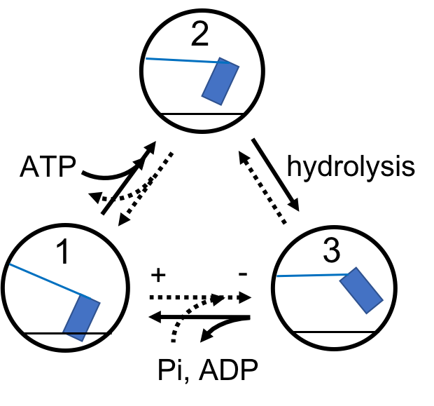
The motor at state 1 is bounded to the actin. Through coupling with an ATP, it detaches and becomes state 2. Then, hydrolysis of ATP leads to the mechanically deformed state 3. Through releasing ADP and Pi, the motor generates a power stroke (from - to +) and re-attach to the actin, back to state 1. The dynamics of this motor (in discrete time) is described by the transition probabilities $P_{j|i}$ from $i$ to $j$, where $i,j\in\left\{1,2,3\right\}$.

With big data about a long trajectory of the motor’s state, we can use counting statistics to infer $P_{j|i}$. Let us consider the following six linearly independent counting frequencies: the occurance frequency of two of the three states, say frequencies $f_{2}$ and $f_{3}$, the symmetric flux (what Maes called traffic in [29]) over all edges measured by

where $ij=\{12,23,13\}$, and the net (antisymmetric) flux of the power stroke step, from state $3$ to $1$, denoted by

Note that this $f_{31}^{{\rm anti}}$ is the net empirical velocity of the motor over a length $T$ trajectory.

Following the MaxEnt recipe mentioned above, we assume a uniform prior $R_{j|i}=1/3$ and construct the tilted matrix

with six parameters $(\alpha_{2},\alpha_{3},\beta_{12},\beta_{23},\beta_{13},\gamma)$ corresponding to the six observables $\boldsymbol{f}=\left(f_{2},f_{3},f_{12}^{{\rm sym}},f_{23}^{{\rm sym}},f_{13}^{{\rm sym}},f_{31}^{{\rm anti}}\right)$. Then by Eq. (8), the posterior transition probabilities take the form of

where $\lambda$ is the largest eigenvalue of $M$ and $r$ is the corresponding right eigenvector.

The set of observables $\boldsymbol{f}$ we chose is holographic, i.e. it captures all degrees of freedom of the dynamics. When the trajectory becomes very long, the ergodic theorem of Markov chain guarantees that $\left(f_{2},f_{3}\right)\rightarrow\left(\pi_{2},\pi_{3}\right)$,

and

With these six averages $\left\langle\boldsymbol{f}\right\rangle=(\pi_{2},\pi_{3},\tau_{12},\tau_{23},\tau_{13},J)$, one can uniquely compute the true underlying $P_{j|i}$ as a function of these six averages. Furthermore, since our observables are non-degenerate, simple relations between the six parameters and the transition probabilities can be derived ¹¹1One of us is writing a paper regarding the general version of this fact.:

where $n=\{2,3\}$ and $ij=\{12,23,13\}$. Notice that $\gamma$ is (half of) the cycle affinity, an important term in stochastic thermodynamics [31].

Recall from Eq. (13) that the six parameters in Eqs. (23) are actually the entropic forces. In our example here, we plug in $R_{j|i}=1/3$ and

into the entropy form $\varphi(\left\langle\boldsymbol{f}\right\rangle)$ in Eq. (9) by using normalization $\pi_{1}=1-\pi_{2}-\pi_{3}$ and stationarity $J_{12}=J_{23}=J_{31}=J$. One can easily check that

for $n=2,3$ and $ij\in\{12,23,31\}$.

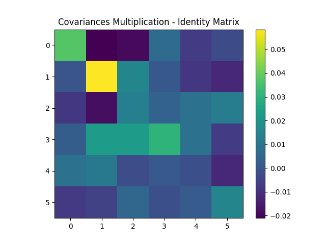
The SUP in Eq. (16) is an asymptotic relation between the covariance of the six frequency observables $\boldsymbol{f}$ collected from a long but finite trajectory and the forces they inferred by computing $\boldsymbol{F}=\nabla\varphi(\boldsymbol{f}).$ By numerically produce a big ensemble of very long trajectories with length $T$, we can play Bob’s role and check the SUP for the empirical $6\times 6$ scaled covariance of frequencies $T{\rm Co\mathbb{V}[\text{$\boldsymbol{f}$}]}$ and that of the inferred forces $T{\rm Co}\mathbb{V}[\boldsymbol{F}]$. Their product is indeed very close to the identify matrix with vanishing difference to the identity matrix shown in Fig. (2).

In this paper, we revisit and advocate the empirical derivation of the Maximum Entropy principle of Markov correlated data [12, 13, 14], also known as the Maximum Caliber principle. We review how the principle can identify entropic forces, and lead to statistical thermodynamic conjugacy. From the empirical understanding and data-driven derivation that we revisited and advocated, we derived an uncertainty principle between the statistical variations of observables and the forces they infer from finite data. This theory is purely empirical and can thus be applied to trajectory data from small, nonequilibrium, dynamical biological systems that are far from mechanics.

In short, more is indeed different [32]. Maximum entropy principle and statistical thermodynamics emerge empirically and de-mechanically from the limit theorems of data ad infinitum, i.i.d. or Markov correlated. Akin to the uncertainty principle in quantum mechanics, there is an uncertainty principle about the statistical variations of dynamical observables and forces for Big Data.