Stellar turbulence and mode physics
Abstract
An overview of selected topical problems on modelling oscillation properties in solar-like stars is presented. High-quality oscillation data from both space-borne intensity observations and ground-based spectroscopic measurements provide first tests of the still-ill-understood, superficial layers in distant stars. Emphasis will be given to modelling the pulsation dynamics of the stellar surface layers, the stochastic excitation processes and the associated dynamics of the turbulent fluxes of heat and momentum.
Keywords asteroseismology; convection; pulsation mode physics; stellar structure.
1 Introduction
With the high-quality photometric data from the Kepler satellite (e.g. Christensen-Dalsgaard et al., 2007) and spectroscopic data from ground-based observation campaigns, and later also from the Danish SONG network (Grundahl et al., 2007), we shall be able to address more carefully many of the current problems in modelling pulsation properties in solar-like stars. In solar-like stars the p-mode lifetimes and amplitudes are crucially affected by the processes that take place in the outer convectively unstable stellar layers. A proper modelling of the dynamics of the convective heat and momentum transfer is therefore essential. Recent 3D numerical simulations of the largest scales of the convection (e.g. Stein & Nordlund, 2001; Samadi et al., 2003; Georgobiani et al., 2004; Stein et al., 2004; Jacoutot et al., 2008; Miesch et al., 2008) have been proven to be extremely useful for calibrating and testing semi-analytical models for convection and stochastic excitation. However, the high-Reynolds-number (and low-Prandtl-number) turbulent convection in stars still prohibits today’s simulations from resolving all the required scales of stellar turbulence. Consequently such simulations have to use sub-grid-scale models, which may lead to different results (e.g. Jacoutot et al., 2008). Because this situation will not change in the near future, we still need analytical models for describing the convection and pulsation dynamics in stars.
Sections 2 and 3 will discuss selected problems of our current understanding of nonadiabatic pulsation dynamics in the Sun and in the hotter F5 star Procyon. Although we can reasonably well reproduce the observed pulsation properties in the Sun, the recent Procyon observations (e.g. Arentoft et al., 2008, and references therein) have revealed serious problems in our models for estimating the oscillation amplitudes in stars hotter than the Sun. In Section 4, therefore, I shall address the problem of selecting a proper temporal turbulence spectrum for modelling the stochastic energy supply rate for acoustic modes.
2 Mode parameters
In solar-like stars all possible modes of oscillation are stable; thus, if a given oscillation mode is somehow excited, its amplitude will decay over a finite time, typically of the order of days to months, the inverse of which is the damping rate . The oscillation power spectrum can be described in terms of an ensemble of intrinsically damped, stochastically driven, simple-harmonic oscillators, provided that the background equilibrium state of the star were independent of time. In that case the mode profile is essentially Lorentzian, and the intrinsic damping rates of the modes could then be determined observationally from measurements of the pulsation linewidths. The other fundamental property of the observed oscillation power spectrum is the height, , of a single peak in the Fourier spectrum. The observed velocity signal (where is the surface displacement of the damped, stochastically driven, harmonic oscillator, and is time) can then be related to the mode height by taking the Fourier transformation of the harmonic oscillator followed by an integration over frequency to obtain the total mean energy in a particular pulsation mode with inertia (e.g. Chaplin et al., 2005; Houdek, 2006). For ,where is observing time, the squared surface rms velocity is then given by
| (1) |
where is the energy supply rate in erg s-1, and is given in units of cms-2Hz-1. The height is the maximum of the discrete power, and is obtained from integrating the power spectral density over a frequency bin:
| (2) |
where is the Fourier transform of , is cyclic frequency, and , is the frequency bin determined by the observation time . It is therefore not the total integrated power, , that is observed directly, but rather the power spectral density (Chaplin et al., 2005).
3 Pulsation amplitude ratios
Linearized pulsation equations for nonadiabatic radial oscillations can be presented as (e.g. Balmforth, 1992a):
| (3) | |||||
| (4) | |||||
| (5) |
where is the Lagrangian perturbation operator, and for simplicity the right hand side of the perturbed momentum equation is formally expressed by the function . Equations (5), together with an equation relating the heat flux to the stratification of the star (the full set of equations can be found in, e.g., Balmforth 1992a), are solved subject to boundary conditions to obtain the eigenfunctions and the complex angular eigenfrequency of the mode , where is the (real) pulsation frequency and the linear damping rate in (s-1). The turbulent flux perturbations of heat and momentum, and , and the fluctuating anisotropy factor are obtained from the nonlocal, time-dependent convection formulation by Gough (1977a, b).
From the linearized nonadiabatic pulsation equations (5) theoretical intensity-velocity amplitude ratios
| (6) |
can be compared with observations, without the need of a specific excitation model and all its uncertainties in describing the turbulence spectrum.
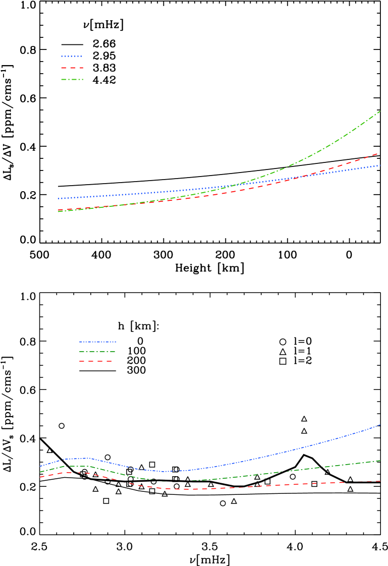
In the top panel of Fig. 1 the theoretical amplitude ratios
(equation (6)) of a solar model are plotted as a function of
height for several radial pulsation modes. The square root of the mode kinetic
energy per unit increment of , which is proportional to
, increases rather slowly with
height; the density , however, decreases very rapidly and consequently
the displacement eigenfunction increases with height. This leads
to the results shown in the upper panel of Fig. 1. The
decrease in the amplitude ratios with height is particularly pronounced for
high-order modes for which the eigenfunctions vary rapidly in the evanescent
outer layers of the atmosphere. It is for that reason why solar velocity
amplitudes from e.g., the GOLF instrument have larger values than the
measurements from the BiSON instrument (by about 25%, Kjeldsen et al. 2005).
The lower panel of Fig. 1 compares the estimated solar
amplitude
ratios (curves) with observed ratios (symbols) as a function of frequency. The
model results are depicted for velocity amplitudes computed at different
atmospheric levels. The observations are obtained from accurate irradiance
measurements from the IPHIR instrument of the PHOBOS 2 spacecraft with
contemporaneous low-degree velocity data from the BiSON instrument at
Tenerife (Schrijver et al., 1991). The thick solid curve represents a
running-mean average, with a width of 300Hz, of the observational data.
The theoretical ratios for km (dashed curve) show reasonable
agreement with the observations.
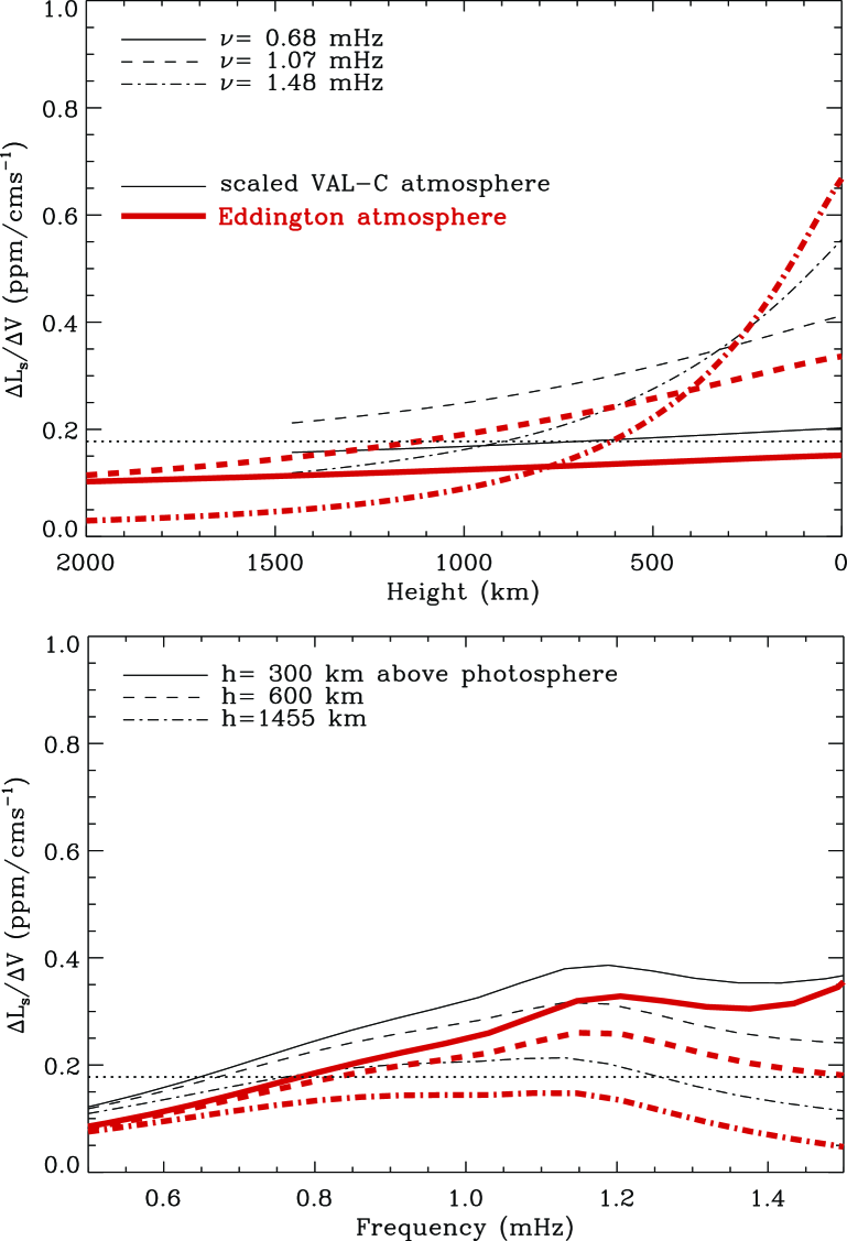
In Fig. 2 model results for the F5 star Procyon A are compared with observations (horizontal dotted line) by Arentoft et al. (2008). Theoretical results are shown for two stellar atmospheres: a VAL-C (Vernazza et al., 1981) atmosphere scaled with the model’s effective temperature (thin curves), and an Eddington atmosphere (thick curves). For both stellar atmospheres the agreement with the observations is less satisfactory than in the solar case, indicating that we may not represent correctly the shape of the pulsation eigenfunctions. Consequently there is need for adopting more realistically computed atmospheres in the equilibrium models, particularly for stars with much higher surface temperatures than the Sun. It should, however, be mentioned that the current photometric observations are still uncertain.
4 Stochastic excitation and turbulent spectra
In solar-like stars the oscillations are driven by the vigorous turbulent convection in the very outer surface layers. The turbulent fluid motion generates acoustic waves in a broad frequency range, which excite a large number of global p modes (of the order of 10 million p modes in the solar case), and possibly also global g modes (e.g. Appourchaux et al., 2009). In the past several stochastic excitation models were proposed (for recent reviews see, e.g. Houdek, 2006; Appourchaux et al., 2009). In general all reported excitation models reproduce reasonably well the observed oscillation amplitudes for solar-like stars that are similar or cooler than the Sun. However, for stars that are somewhat hotter than the Sun, theoretical predictions overestimate the pulsation amplitudes by up to a factor of about four, such as for the F5 star Procyon A. Additional to the uncertainties in modelling the shape of the pulsation eigenfunctions in the atmospheric stellar layers (see Section 3), modelling of the mode damping rates (see e.g., Houdek, 2006) and the turbulent energy spectrum play also a crucial role in estimating the mode amplitudes. In this paper I shall only address the problem of modelling the turbulent spectrum for estimating the energy supply rate .
4.1 Stochastic excitation model
A review on this topic was recently given by Appourchaux et al. (2009). Therefore I shall summarize only the most important matters. According to Eq. (1) we need to model the (linear) damping rate and the energy supply rate for estimating the mode height . In this paper I shall address only the modelling of the energy supply rate. One of the problems that one faces in deriving a stochastic excitation model is the separation of the total fluid motion into (large-scale) oscillatory motion (oscillation modes), with displacement , and small-scale turbulent motion with the convective velocity field . This separation is superficially straightforward for radial p modes (Gough, 1977a); however, for nonradial modes this separation is a much more difficult task and can possibly not be accomplished for the very-high-degree p modes and also very-high-order g modes (see e.g. Appourchaux et al., 2009). For simplicity we shall discuss here only radial p modes.
Following the basic principle of Lighthill’s acoustic analogy (Lighthill, 1952, see also Crighton 1975) one typically arranges the linearized global mode variables on the left and the nonlinear fluctuating terms associated with the turbulent convection on the right of the equations of motion, which may then be written as
| (7) |
in which the linear spatial differential operator satisfies the (unforced) homogeneous wave equation for the mode eigenfunctions with frequencies , and is the nonlinear stochastic forcing and damping term that depends only on the turbulent velocity field . Here we consider only the Reynolds stress driving term, which dominates over the entropy driving term in the Sun and in most solar-type stars (Balmforth, 1992b; Stein & Nordlund, 2001; Stein et al., 2004; Belkacem et al., 2006; Samadi et al., 2007). It should, however, be noted that there is partial cancellation between the fluctuating Reynolds stress and entropy source terms, which could lead to smaller oscillation amplitudes than adopting the Reynolds stress contribution alone (Osaki, 1990; Stein et al., 2004; Houdek, 2006). Because the mode amplitudes of solar-type oscillations are small it is additionally assumed that they do not interact with the nonlinear right hand side of the wave equation, and consequently one can solve Eq. (7) by a nonsingular perturbation method (Goldreich & Keeley, 1977; Balmforth, 1992b; Samadi & Goupil, 2001; Chaplin et al., 2005). For radial modes only the vertical component of the fluctuating Reynolds stress source term is important,
| (8) |
which depends on the component of a two-point correlation function, , where angular brackets denote an ensemble average. For incompressible, homogeneous isotropic turbulence the Fourier transform of is proportional to the turbulent energy spectrum function , i.e.
| (9) |
(Batchelor, 1953), where is a wavenumber.
Following Stein (1967) we factorize the energy spectrum function into , where
| (10) |
is the correlation time-scale of eddies with vertical size and velocity ; the correlation factor is of order unity and accounts for uncertainties in defining . For statistically stationary turbulence the energy supply rate is then given by (see e.g., Chaplin et al. 2005 for details)
| (11) |
with
| (12) |
where is the component of the (mean) Reynolds stress tensor, , is surface radius, is the normalized radial part of , and the product of and is a factor of unity accounting for the anisotropy of the turbulent velocity field. The spectral function accounts for contributions to from the small-scale turbulence. For the normalized spatial turbulence energy spectrum it has been common to adopt, for example, the Kolmogorov (1941) spectrum. For the frequency-dependent factor , however, which is used for evaluating the self-convolution in Eq. (12), no satisfactory theory exists. Various functional forms were proposed in the past, which lead, however, to rather different values for the modelled oscillation amplitudes (Samadi et al., 2003; Chaplin et al., 2005; Appourchaux et al., 2009). We shall therefore discuss the most commonly adopted frequency-dependent factors for stellar turbulence spectra in the next section.
4.2 Turbulence spectra
Differences in the (properly normalized) spatial spectrum
create only minor differences in the energy supply rate
(e.g., Balmforth, 1992b; Samadi & Goupil, 2001; Chaplin et al., 2005). But differences in the
frequency-dependent (temporal) spectrum would create
rather large differences in the p-mode and also g-mode amplitudes
(Samadi et al., 2003; Chaplin et al., 2005; Belkacem et al., 2009; Appourchaux et al., 2009). Those differences
are produced by the convection-oscillation interactions in the deeper
convectively unstable stellar layers, which are off resonance, and whose
magnitude depends crucially on the adopted frequency dependence of the
turbulence spectrum in the high-frequency tail of the cascade.
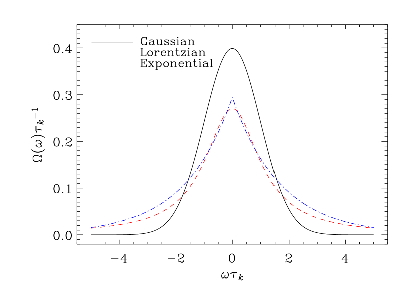
We consider the following factors:
(i) the Exponential factor (Stein, 1967)
| (13) |
(ii) the Gaussian factor (Stein, 1967)
| (14) |
(iii) the Lorentzian factor (Gough, 1977a; Samadi et al., 2003; Chaplin et al., 2005)
| (15) |
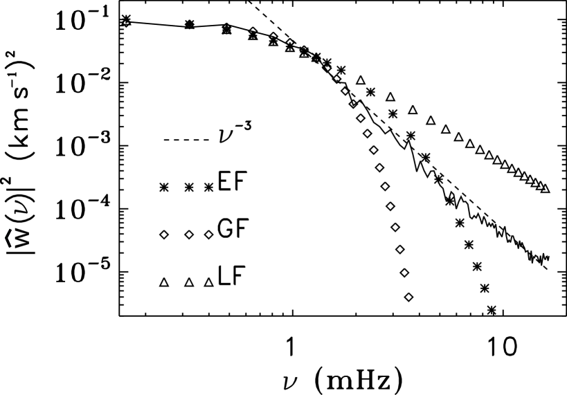
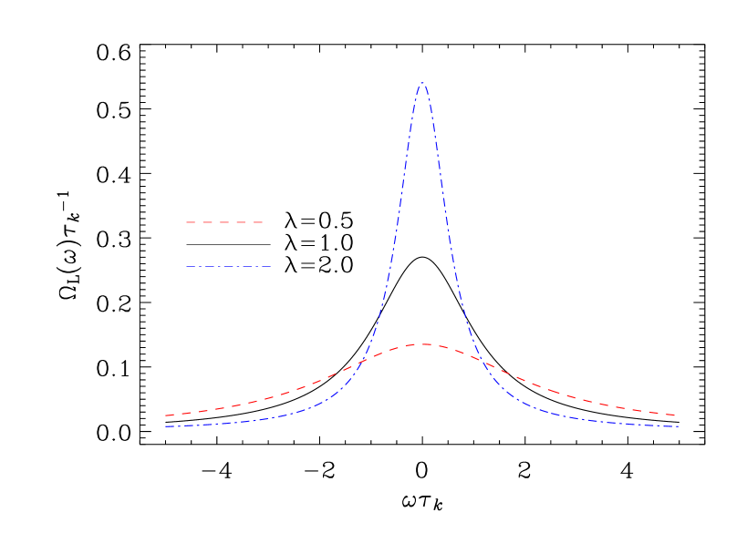
Fig. 3 compares the dimensionless quantity for the three frequency factors (13)–(15). All three factors are normalized according to , the integral being from to . Furthermore, the full-width at half-maximum, i.e. , has been chosen to be the same for all three factors, in order to have a meaningful comparison. The Gaussian frequency factor decreases more rapidly with , than both the Exponential and Lorentzian factors, i.e. the Gaussian factor produces the smallest magnitude in the high-frequency tail of the spectrum. Convective eddies situated in the deeper convectively unstable stellar layers have longer characteristic time scales , i.e. [see Eq. (10)] increases with depth in the star (see for example Fig. 5 of Chaplin et al., 2005). The Lorentzian factor decreases more slowly with depth at constant frequency and consequently a larger fraction of the integrands of Eqs (11) and (12) arises from large off-resonant eddies situated deep in the star, whereas the Gaussian frequency factor gives less weight to the large off-resonance eddies. As a result of this the modelled oscillation amplitudes are larger with a Lorentzian time-correlation function and therefore in better agreement with the observations than with a Gaussian (Samadi et al., 2003, 2007). However, Chaplin et al. (2005) reported that the Lorentzian time-correlation function leads to overestimated heights at low frequencies for solar p modes. Also for solar g modes Belkacem et al. (2009) concluded that the best fit for reproducing the observations was obtained with a Gaussian factor at the lowest and a Lorentzian at the highest frequencies. Moreover, Belkacem et al. (2009) reported that the correlation parameter [see Eq. (10)] has to increase with stellar depth in order to reproduce the 3D numerical simulations by Miesch et al. (2008), a result that is consistent with the findings by Chaplin et al. (2005). The effect of on the time-correlation functions is demonstrated in Fig. 4 for a Lorentzian factor. Increasing leads to a more rapidly declining tail and consequently to a smaller contribution to the energy supply rate from the off-resonant eddies situated in the deep convection zone. Finding the correct time-correlation function for stellar turbulence remains an open issue.
From the theoretical point of view a Lorentzian factor is a result predicted for the largest, most-energetic eddies by the time-dependent mixing-length formulation of Gough (1977a). Moreover, in agreement with Kolmogorov (1941) theory Sawford (1991) demonstrated that in the limit of high-Reynolds-number turbulence the two-point velocity autocorrelation, normalized by the velocity variance , is
| (16) |
where
| (17) |
is the Lagrangian integral time scale (see also Legg & Raupach, 1982). Consequently the normalized velocity autocorrelation is proportional to an exponential decrease with separation time in the inertial range, and the velocity spectrum becomes with Eq. (16)
| (18) | |||||
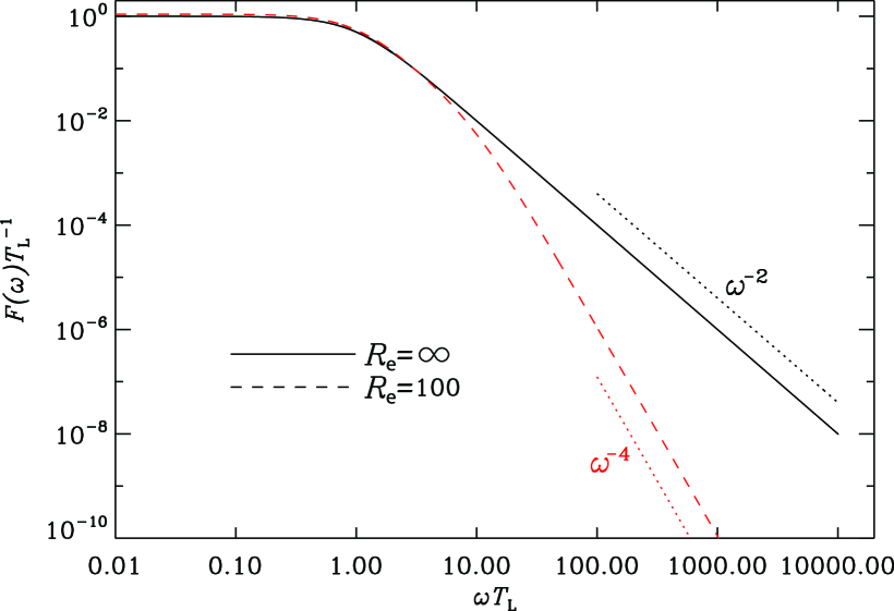
i.e. it is of Lorentzian shape with for and at infinite Reynolds number . Sawford extended this analysis for arbitrary values of the Reynolds number , where and are the time scales of the energy-containing eddies and the Kolmogorov timescale respectively (Tennekes & Lumley, 1972). For this case the velocity spectrum is (Sawford, 1991)
| (19) |
Fig. 5 displays the spectrum of the normalized velocity autocorrelation for two different values of the Reynolds number, . It is interesting to note that there is essentially no inertial range with a frequency decay of , i.e. a Lorentzian frequency dependence [Eq. (18)], for ; the spectrum decreases as in the dissipation subrange, i.e. for turbulent scales close to the Kolmogorov dissipation scale.
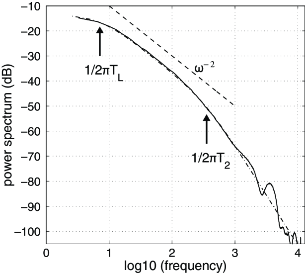
These findings are supported by laboratory experiments. Fig. 6 displays the measured velocity power spectrum in a rotating shear turbulence experiment (Kàrmàn swirling flow) with water. The solid curve displays the measurements and the dot-dashed curve is a fit of expression (19) to the data with , where and . There is a well defined inertial range for frequencies between and with a decay of about , i.e. a Lorentzian spectrum. The high-frequency tail, however, decays more rapidly. The measurements are superficially similar to the second-order model by Sawford (1991) depicted in Fig. 5. It should, however, be noted that the molecular Prandtl number of about 6.8 in the water experiment is several magnitudes larger than the molecular Prandtl number in stellar convection zones, which is typically of order .
Georgobiani et al. (2004) used, as did Samadi et al. (2003), the 3D Large-Eddy-Simulations by Stein & Nordlund (2001) to investigate the time-correlation function in the Sun. Fig. 7 compares the power spectrum (squared fast Fourier transform), , of the vertical component of the turbulent velocity field, , at fixed horizontal wavenumber and depth, between the simulation results (solid curve) and various analytical time-correlation functions [Exponential (EF), Gaussian (GF) and Lorentzian (LF) frequency factors]. The results are shown for a wavenumber Mm-1 computed 250 km below the solar surface. Neither of the three analytical functions fit the simulation results, particularly in the high-frequency tail of the spectrum. Moreover, Georgobiani et al. (2004) reported that the functional form (frequency dependence) of the simulation results changes substantially with wavenumber and depth, and consequently that the turbulent energy spectrum function is not separable into wavenumber and frequency . The authors suggest using instead the following empirical function for the temporal part of the vertical velocity power spectrum
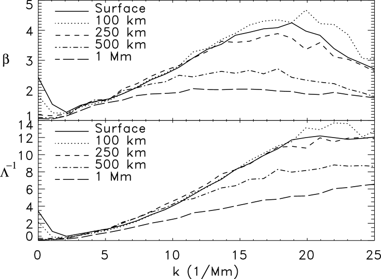
| (20) |
where the two coefficients and are determined from fitting Eq. (20) to the 3D simulation results. Note that for a Lorentzian frequency factor is recovered. Results from solar simulations are given in Fig. 8 for various horizontal wavenumbers and depths. In agreement with Chaplin et al. (2005) and Belkacem et al. (2009) the coefficient increases with depth, i.e. the width of the frequency factor decreases with depth (see also Fig. 4), particularly at smaller scales (i.e. at large wavenumbers). Except near the surface the values of the exponent are rather larger than unity.
4.3 Effect of sub-grid models on simulation results
Numerical simulations of stellar convection resolve only the largest scales
of the turbulent motion. The smaller scales still need to be approximated
by a so-called sub-grid model. Such simulations are called
Large-Eddy-Simulations. The total number of scales that are numerically
resolved, i.e. the ratio of the largest scale to the smaller scale
, is related to the Reynolds number by (e.g. Tennekes & Lumley, 1972)
and consequently the total number of grid points in
the simulation is
A solar Reynolds number of
would require a total meshpoint number
of . With today’s super computers the maximum achievable number
of meshpoints is , and is therefore some
15 magnitudes too small for what is required to resolve all the turbulent
scales of solar convection. Consequently a sub-grid model is necessary for
describing the dynamics of the numerically unresolved smaller scales of
the turbulent cascade.
Various models are available. The most commonly used models are hyperviscosity
models and the Smagorinsky model. All sub-grid models assume that turbulent
transport is a diffusive process. Hyperviscosity models, for example, use
higher derivatives for the diffusion operator in the momentum equation,
thereby extending the inertial range, which also leads to a better
representation of the dynamics of the larger scales. An overview of
sub-grid models was recently presented by Miesch (2005).
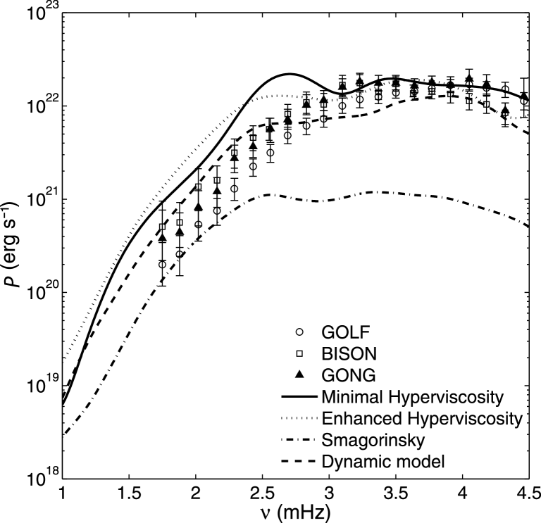
An obvious question to ask is what are the effects of using different
sub-grid models on the mode properties in simulations of solar-type stars?
This question was recently addressed, in part, by Jacoutot et al. (2008), who
compared simulated solar energy supply
rates using various sub-grid models. Their results are summarized in
Fig. 9. Agreement with observations is generally
satisfactory except for the classical Smagorinsky model.
It is also important to note that the Prandtl number in 3D simulations is currently about 0.01 0.25 (e.g. Miesch et al., 2008). It is therefore substantially larger than the Prandtl number in the Sun and in solar-type stars. Although numerical simulations provide an important input to our understanding of stellar convection and are very important for calibrating semi-analytical convection models, we must remain aware of the shortcomings of the currently used 3D numerical simulations.
Acknowledgements I am very grateful to Douglas Gough for many helpful discussions. Support by the Austrian Science Fund (FWF project P21205) is thankfully acknowledged.
References
- Appourchaux et al. (2009) Appourchaux T., Belkacem K., Broomhall A.-M., Chaplin W.C., Gough D.O., Houdek G., Provost J., et al. 2009, Astron. Astrophys. Rev., in the press (arXiv:0910.0848)
- Arentoft et al. (2008) Arentoft T., Kjeldsen H., Bedding T.R., Bazot M., Christensen-Dalsgaard J., Dall T.H., Karoff C., Carrier F. et al. 2008, Astron. J. 687, 1180
- Balmforth (1992a) Balmforth N.J. 1992a, Mon. Not. R. Astron. Soc. 255, 603
- Balmforth (1992b) Balmforth N.J. 1992b, Mon. Not. R. Astron. Soc. 255, 639
- Batchelor (1953) Batchelor G.K. 1953, Homogeneous Turbulence, Cambridge University Press, Cambridge
- Belkacem et al. (2006) Belkacem K., Samadi R., Goupil M.-J., Kupka F., Baudin F. 2006, Astron. Astrophys. 460, 183
- Belkacem et al. (2009) Belkacem K., Samadi R., Goupil M.-J., Dupret M.-A., Brun A.S., Baudin F. 2009, Astron. Astrophys. 494, 191
- Chaplin et al. (2005) Chaplin W., Houdek G., Elsworth Y., Gough D.O., Isaac G.R., New R., 2005, Mon. Not. R. Astron. Soc. 360, 859
- Christensen-Dalsgaard et al. (2007) Christensen-Dalsgaard J., Arentoft T., Brown T.M., Gilliland R.L., Kjeldsen H., Borucki W.J., Koch D. 2007, In Future of Asteroseismology, eds Handler G., Houdek G., Comm. Asteroseis. 150, p. 350
- Crighton (1975) Crighton D.G. 1975, Progess in Aerospace Science 16, 31
- Georgobiani et al. (2004) Georgobiani D., Stein R.F., Nordlund Å. 2004, In Solar MHD Theory and Observations, eds Leibacher J., Stein R.F., Uitenbroek H., ASP Conf. Ser., Vol. 354, p. 109
- Goldreich & Keeley (1977) Goldreich P., Keeley D.A. 1977, Astrophys. J. 212, 243
- Gough (1977a) Gough D.O. 1977a, Astrophys. J. 214, 196
- Gough (1977b) Gough D.O. 1977b, In: Problems of Stellar Convection, eds Spiegel E.A., Zahn J.-P., Springer-Verlag, Berlin, p. 15
- Grundahl et al. (2007) Grundahl F., Kjeldsen H., Christensen-Dalsgaard J., Arentoft T., Frandsen S., 2007, in: Future of Asteroseismology, eds Handler G., Houdek G., Comm. Asteroseis. 150, p. 300
- Houdek (2006) Houdek G. 2006, In SOHO18/ GONG 2006/HelAs I: Beyond the spherical Sun, Fletcher K., Thompson M.J., eds, ESA SP-624, Noordwijk, p. 28.1
- Houdek et al. (1999) Houdek G., Balmforth N.J., Christensen-Dalsgaard J., Gough D.O., Astron. Astrophys. 1999, 351, 582
- Jacoutot et al. (2008) Jacoutot L., Kosovichev A.G., Wray A.A., Mansour N.N. 2008, Astrophys. J. 682, 1386
- Kjeldsen et al. (2005) Kjeldsen H., Bedding T.R., Butler R.P., et al. 2005, Astrophys. J. 635, 1281
- Kolmogorov (1941) Kolmogorov A.N. 1941, Dokl. Akad. Nauk SSSR, 30, 299
- Legg & Raupach (1982) Legg B.J., Raupach M.R. 1982, Boundary-Layer Meteorology 24, 3
- Lighthill (1952) Lighthill M.J. 1952, Proc. Roy. Soc. A 211, 564
- Miesch (2005) Miesch M.S. 2005, Living Reviews in Solar Physics 2, Online: http://www.livingreviews.org/lrsp-2005-1
- Miesch et al. (2008) Miesch M.S. Brun A.S., DeRosa M.L., Toomre J. 2008, Astrophys. J. 673, 557
- Mordant et al. (2004) Mordant N., Lévêque, E., Pinton J.-F. 2004, New Journal of Physics 6, 116
- Osaki (1990) Osaki Y. 1990, In Progress of Seismology of the Sun and Stars, eds Y. Osaki Y., H. Shibahashi, Springer-Verlag, Berlin, p. 145
- Samadi & Goupil (2001) Samadi R., Goupil M.-J. 2001, Astron. Astrophys. 370, 136
- Samadi et al. (2003) Samadi R., Nordlund Å., Stein R.F., Goupil M.-J., Roxburgh I. 2003, Astron. Astrophys. 404, 1129
- Samadi et al. (2007) Samadi R., Georgobiani D., Trampedach R., et al. Astron. Astrophys. 463, 297
- Sawford (1991) Sawford B.L. 1991, Phys. Fluids A 3(6), 1577
- Schrijver et al. (1991) Schrijver C.J., Jiménez A., Däppen W. 1991, Astron. Astrophys. 251, 655
- Stein (1967) Stein R.F. 1967, Sol. Phys. 2, 385
- Stein & Nordlund (2001) Stein R.F., Nordlund Å. 2001, Astrophys. J. 546, 585
- Stein et al. (2004) Stein R., Georgobiani D., Trampedach R., Ludwig H.-G., Nordlund Å. 2004, Sol. Phys. 220, 229
- Tennekes & Lumley (1972) Tennekes H., Lumley J.L. 1972, A first Course in Turbulence, MIT Presse, Cambridge, Massachusetts
- Vernazza et al. (1981) Vernazza J.E., Avrett E.H., Loeser R. 1981, ApJS 45, 635