Stochastic Dynamics of Noisy Average Consensus: Analysis and Optimization
Abstract
A continuous-time average consensus system is a linear dynamical system defined over a graph, where each node has its own state value that evolves according to a simultaneous linear differential equation. A node is allowed to interact with neighboring nodes. Average consensus is a phenomenon that the all the state values converge to the average of the initial state values. In this paper, we assume that a node can communicate with neighboring nodes through an additive white Gaussian noise channel. We first formulate the noisy average consensus system by using a stochastic differential equation (SDE), which allows us to use the Euler-Maruyama method, a numerical technique for solving SDEs. By studying the stochastic behavior of the residual error of the Euler-Maruyama method, we arrive at the covariance evolution equation. The analysis of the residual error leads to a compact formula for mean squared error (MSE), which shows that the sum of the inverse eigenvalues of the Laplacian matrix is the most dominant factor influencing the MSE. Furthermore, we propose optimization problems aimed at minimizing the MSE at a given target time, and introduce a deep unfolding-based optimization method to solve these problems. The quality of the solution is validated by numerical experiments.
I Introduction
Continuous-time average consensus system is a linear dynamical system defined over a graph [3]. Each node has its own state value, and it evolves according to a simultaneous linear differential equation where a node is only allowed to interact with neighboring nodes. The ordinary differential equation (ODE) at the node governing the evolution of the state value of the node is given by
| (1) |
The set denote the neighboring nodes of node , while the positive scalar denotes the edge weight associated with the edge . The same ODE applies to all other nodes as well. These dynamics gradually decrease the differences between the state values of neighboring nodes, leading to a phenomenon called average consensus that the all the state values converge to the average of the initial state values [2].
The average consensus system has been studied in numerous fields such as multi-agent control [4], distributed algorithm [5], formation control [6]. An excellent survey on average consensus systems can be found in [3].
In this paper, we will examine average consensus systems within the context of communications across noisy channels, such as wireless networks. Specifically, we consider the scenario in which nodes engage in local wireless communication, such as drones flying in the air or sensors dispersed across a designated area. It is assumed that each node can only communicate with neighboring nodes via an additive white Gaussian noise (AWGN) channel. The objective of the communication is to aggregate the information held by all nodes through the application of average consensus systems. As previously stated, the consensus value is the average of the initial state values.
In this setting, we must account for the impact of Gaussian noise on the differential equations. The differential equation for a noisy average consensus system takes the form:
| (2) |
where represents an additive white Gaussian process, and is a positive constant. The noise can be considered as the sum of the noises occurring on the edges adjacent to the node . In a noiseless average consensus system, it is well-established that the second smallest eigenvalue of the Laplacian matrix of the graph determines the convergence speed to the average [5]. The convergence behavior of a noisy system may be quite different from that of the noiseless system due to the presence of edge noise. However, the stochastic dynamics of such a system has not yet been studied. Studies on discrete-time consensus protocols subject to additive noise can be found in [11][12], but to the best of our knowledge, there are no prior studies on continuous-time noisy consensus systems.
The main goal of this paper is to study the stochastic dynamics of continuous-time noisy average consensus system. The theoretical understanding of the stochastic behavior of such systems will be valuable for various areas such as multi-agent control and the design of consensus-based distributed algorithms for noisy environments.
The primary contributions of this paper are as follows. We first formulate the noisy average consensus systems using stochastic differential equations (SDE) [7][8]. This SDE formulation facilitates mathematically rigorous treatment of noisy average consensus. We use the Euler-Maruyama method [7] for solving the SDE, which is a numerical method for solving SDEs. We derive a closed-form mean squared error (MSE) formula by analyzing the stochastic behavior of the residual errors in the Euler-Maruyama method. We show that the MSE is dominated by the sum of the inverse eigenvalues of the Laplacian matrix. However, minimizing the MSE at a specific target time is a non-trivial task because the objective function involves the sum of the inverse eigenvalues. To solve this optimization problem, we will propose a deep unfolding-based optimization method.
The outline of the paper is as follows. In Section 2, we introduce the mathematical notation used throughout the paper, and then provide the definition and fundamental properties of average consensus systems. In Section 3, we define a noisy average consensus system as a SDE. In Section 4, we present an analysis of the stochastic behavior of the consensus error and derive a concise MSE formula. In Section 5, we propose a deep unfolding-based optimization method for minimizing the MSE at a specified target time. Finally, in Section 6, we conclude the discussion.
II Preliminaries
II-A Notation
The following notation will be used throughout this paper. The symbols and represent the set of real numbers and the set of positive real numbers, respectively. The one dimensional Gaussian distribution with mean and variance is denoted by . The multivariate Gaussian distribution with mean vector and covariance matrix is represented by . The expectation operator is denoted by . The notation is the diagonal matrix whose diagonal elements are given by . The matrix exponential is defined by
| (3) |
The Frobenius norm of is denoted by . The notation denotes the set of consecutive integers from to .
II-B Average Consensus
Let be a connected undirected graph where . Suppose that a node can be regarded as an agent communicating over the graph . Namely, a node and a node can communicate with each other if . We will not distinguish and because the graph is undirected.
Each node has a state value where represents continuous-time variable. The neighborhood of a node is represented by
| (4) |
Note that the node is excluded from . For any time , a node can access the self-state and the state values of its neighborhood, i.e., but cannot access to the other state values.
In this section, we briefly review the basic properties of the average consensus processes [3]. We now assume that the set of state values are evolved according to the simultaneous differential equations
| (5) |
where the initial condition is
| (6) |
The edge weight follows the symmetric condition
| (7) |
Let be a degree sequence where is defined by
| (8) |
The continuous-time dynamical system (5) is called an average consensus system because a state value converges to the average of the initial state values at the limit of , i.e,
| (9) |
where the vector represents and is defined by
| (10) |
We define the Laplacian matrix of this consensus system as follows:
| (11) | ||||
| (12) | ||||
| (13) |
From this definition, a Laplacian matrix satisfies
| (14) | ||||
| (15) | ||||
| (16) |
Note that the eigenvalues of the Laplacian matrix are nonnegative real because is a positive semi-definite symmetric matrix. Let be the eigenvalues of and be the corresponding orthonormal eigenvectors. The first eigenvector is corresponding to the eigenvalue , which results in .
By using the notion of the Laplacian matrix, the dynamical system (5) can be compactly rewritten as
| (17) |
where the initial condition is . The dynamical behaviors of the average consensus system (17) are thus characterized by the Laplacian matrix . Since the ODE (17) is a linear ODE, it can be easily solved. The solution of the ODE (17) is given by
| (18) |
Let where is an orthogonal matrix. The Laplacian matrix can be diagonalized by using , i.e.,
| (19) |
On the basis of the diagonalization, we have the spectral expansion of the matrix exponential:
| (20) |
Substituting this to , we immediately have
| (21) |
The second term of the right-hand side converges to zero since for . This explains why average consensus happens, i.e., the convergence to the average of the initial state values (9). The second smallest eigenvalue , called algebraic connectivity [10], determines the convergence speed because shows the slowest convergence in the second term.
III Noisy average consensus system
III-A SDE formulation
The dynamical model (2) containing a white Gaussian noise process is mathematically challenging to handle. We will use a common approach of approximating the white Gaussian process by using the standard Wiener process. Instead of model (2), we will focus on the following stochastic differential equation (SDE) [8]
| (22) |
to study the noisy average consensus system. The parameter is a positive real number, and it represents the intensity of the noises. The stochastic term represents the -dimensional standard Wiener process. The elements of are independent one dimensional-standard Wiener processes. For the Wiener process , we have , , and it satisfies
| (23) |
III-B Approaches for studying stochastic dynamics
Our primary objective in the following analysis is to investigate the stochastic dynamics of the noisy average consensus system, focusing on deriving the mean and covariance of the solution for the SDE (22).
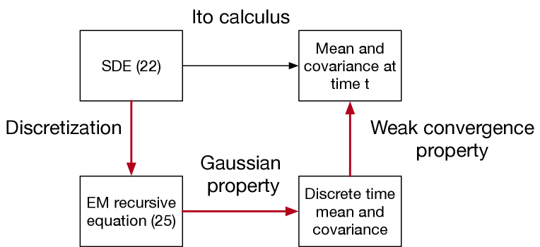
There are two approaches to analyze the system. The first approach relies on the established theory of Ito calculus [8], which is used to handle stochastic integrals directly (see Fig. 1). Ito calculus can be applied to derive the first and second moments of the solution of (22).
Alternatively, the second approach employs the Euler-Maruyama (EM) method [7] and utilizes the weak convergence property [7] of the EM method. We will adopt the latter approach in our analysis, as it does not require knowledge of advanced stochastic calculus if we accept the weak convergence property. Additionally, this approach can be naturally extended to the analysis on the discrete-time noisy average consensus system. Furthermore, the EM method plays a key role in the optimization method to be presented in Section V. Our analysis motivates the use EM method for optimizing the covariance.
III-C Euler-Maruyama method
We use the Euler-Maruyama method corresponding to this SDE so as to study the stochastic behavior of the solution of the SDE (22) defined above. The EM method is well-known numerical method for solving SDEs [7].
Assume that we need numerical solutions of a SDE in the time interval . We divide this interval into bins and let where the interval is given by Let us define a discretized sample be It should be noted that, the choice of the width is crucial in order to ensure the stability and the accuracy of the EM method. A small width leads to a more accurate solution, but requires more computational time. A large width may be computationally efficient but may lead to instability in the solution.
The recursive equation of the EM method corresponding to SDE (22) is given by
| (24) |
where each element of follows In the following discussion, we will use the equivalent expression [7]:
| (25) |
where is a random vector following the multivariate Gaussian distribution . The initial vector is set to be . This recursive equation will be referred to as the Euler-Maruyama recursive equation.
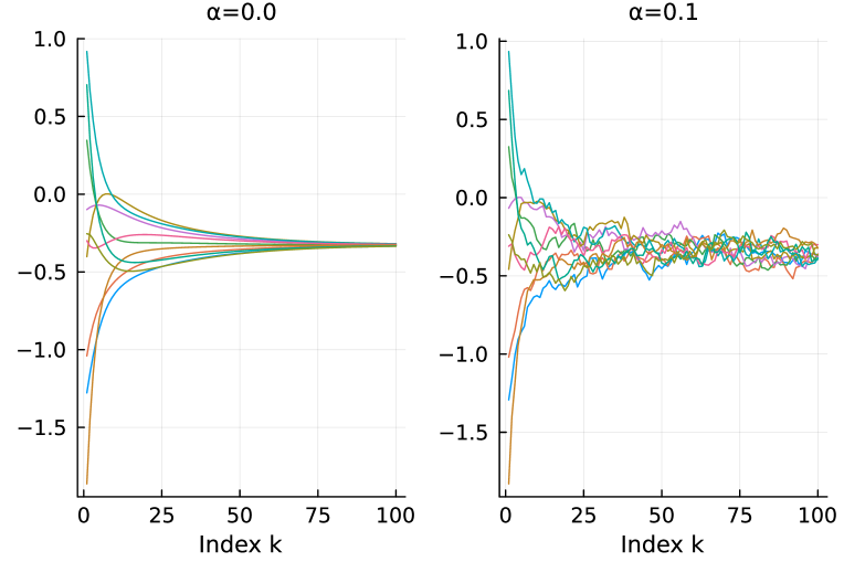
Figure 2 presents a solution evaluated with the EM method. The cycle graph with 10 nodes with the degree sequence is assumed. The initial value is randomly initialized as . We can confirm that the state values are certainly converging to the average value in the case of noiseless case (left). On the other hand, the state vector fluctuates around the average in the noisy case (right).
IV Analysis for Noisy average consensus
IV-A Recursive equation for residual error
In the following, we will analyze the stochastic behavior of the residual error. This will be the basis for the MSE formula to be presented.
Recall that the initial state vector is and that the average of the initial values is denoted by . Since the set of eigenvectors of is an orthonormal base, we can expand the initial state vector as
| (26) |
where the coefficient is obtained by . Note that holds.
At the initial index , the Euler-Maruyama recursive equation becomes
| (27) |
Substituting (26) into the above equation, we have
| (28) |
where the equations and are used in the last equality. Subtracting from the both sides, we get
| (29) |
For the index , the Euler-Maruyama recursive equation can be written as
| (30) |
Subtracting from the both sides, we have
| (31) |
By using the relation we can rewrite the above equation as
| (32) |
It can be confirmed the above recursion (32) is consistent with the initial equation (29). We here summarize the above argument as the following lemma.
Lemma 1
Let be the residual error at index . The evolution of the residual error of the EM method is described by
| (33) |
for .
The residual error denotes the error between the average vector and the state vector at time index . By analyzing the statistical behavior of , we can gain insight into the stochastic properties of the dynamics of the noisy consensus system.
IV-B Asymptotic mean of residual error
Let a vector . Recall that the vector obtained by a linear map also follows the Gaussian distribution, i.e.,
| (34) |
where . If two Gaussian vectors and are independent, the sum becomes also Gaussian, i.e,
| (35) |
In the recursive equation (33), it is evident that follows a multivariate Gaussian distribution because
| (36) |
is the sum of a constant vector and a Gaussian random vector. From the above properties of Gaussian random vectors, the residual error vector follows the multivariate Gaussian distribution where the mean vector and the covariance matrix are recursively determined by
| (37) | ||||
| (38) |
for where the initial values are formally given by
| (39) | ||||
| (40) |
Solving the recursive equation, we can get the asymptotic mean formula as follows.
Lemma 2
Suppose that is given. The asymptotic mean at is given by
| (41) |
(Proof) The mean recursion is given as for . Recall that the eigenvalue decomposition of is given by . From
| (42) |
we have
| (43) |
This implies, from the definition of exponential function,
| (44) |
where .
It is easy to confirm that the claim of this lemma is consistent with the continuous solution of noiseless case (18). Namely, at the limit of , the state evolution of the noisy system converges to that of the noiseless system.
IV-C Asymptotic covariance of residual error
We here discuss the asymptotic behavior of the covariance matrix at the limit of .
Lemma 3
Suppose that is given. The asymptotic covariance matrix at is given by
| (45) |
where is defined by
| (46) |
(Proof) Recall that
| (47) |
Let . A spectral representation of the covariance evolution (38) is thus given by
| (48) |
where . The first component follows a recursion and thus we have Another component follows
| (49) |
Let us consider the characteristic equation of (49) which is given by
| (50) |
The solution of the equation is given by
| (51) |
The above recursive equation (49) thus can be transformed as
| (52) |
From the above equation, can be solved as
| (53) |
Taking the limit , we have
| (54) |
We thus have the claim of this lemma.
IV-D Weak convergence of Euler-Maruyama method
As previously noted, the asymptotic mean (41) is consistent with the continuous solution. The weak convergence property of the EM method [7] allows us to obtain the moments of the error at time .
We will briefly explain the weak convergence property. Suppose a SDE with the form:
| (55) |
If and are bounded and Lipschitz continuous, then the finite order moment estimated by the EM method converges to the exact moment of the solution at the limit [7]. This property is called the weak convergence property. In our case, the SDE (22) has bounded and Lipschitz continuous coefficient functions, i.e, and . Hence, we can employ the weak convergence property in our analysis.
Suppose is a solution of SDE (22) with the initial condition . Let be the mean vector of the residual error and is the covariance matrix of the residual error .
Theorem 1
For a positive real number , the mean and the covariance matrix of the residual error are given by
| (56) | ||||
| (57) |
(Proof) Due to the weak convergence property of the EM method, the first and second moments of the error are converged to the asymptotic mean and covariance of the EM method [7], i.e.,
| (58) | ||||
| (59) |
where and are related by . Applying Lemmas 2 and 3 and replacing the variable by provide the claim of the theorem.
IV-E Mean squared error
In the following, we assume that the initial state vector follows Gaussian distribution .
In this setting, also follows multivariate Gaussian distribution with the mean vector and the covariance matrix where
| (60) |
because can be rewritten as
| (61) |
By using the result of Theorem 1, we immediately have the following corollary indicating the MSE formula.
Corollary 1
The mean squared error (MSE)
| (62) |
is given by
(Proof) We can rewrite as:
| (63) |
where , and and are independent. We thus have
| (64) |
due to Theorem 1.
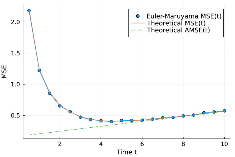
Since the value of the term is exponentially decreasing with , is dominant in for sufficiently large . For sufficiently large , the MSE is well approximated by the asymptotic MSE (AMSE) as
| (65) |
because is negligible, and can be well approximated to . We can observe that the sum of inverse eigenvalue of the Laplacian matrix determines the intercept of the . In other words, the graph topology influences the stochastic error behavior through the sum of inverse eigenvalues of the Laplacian matrix.
Figure 3 presents a comparison of evaluated by the EM method (25) and the formula in (64). In this experiment, the cycle graph with 10 nodes is used. The values of are also included in Fig. 3. We can see that the theoretical values of and estimated values by the EM method are quite close.
V Minimization of mean squared error
V-A Optimization Problems A and B
In the previous section, we demonstrated that the MSE can be expressed in closed-form. It is natural to optimize the edge weights in order to decrease the value of the MSE. The optimization of the edge weights is equivalent to the optimization of the Laplacian matrix . There exist several related works that aim to achieve a similar goal for noise-free systems. For example, Xiao and Boyd [5] proposed a method to minimize the second eigenvalue to achieve the fastest convergence to the average. They formulated the optimization problem as a convex optimization problem, which can be solved efficiently. Kishida et al. [13] presented a deep unfolding-based method for optimizing time-dependent edge weights, yet these methods are not applicable to systems with noise. Optimizing the MSE may be a non-trivial task as it involves the sum of the inverse eigenvalues of the Laplacian matrix.
In this subsection, we will present two optimization problems of edge weights.
V-A1 Optimization problem A
Assume that a degree sequence is given in advance. The optimization problem A is the minimization problem of under the given degree sequence where is the predetermined target time given in advance. The precise formulation of the problem is given as follows:
| subject to: | ||||
| (66) | ||||
| (67) | ||||
| (68) | ||||
| (69) | ||||
| (70) | ||||
The constraint (67) is imposed for the symmetry of the edge weight for . The row sum constraint (68) is needed for satisfying (8). The constraint (69) means that should be close enough to the given degree sequence. The positive constant can be seen as a tolerance parameter.
One way to interpret the optimization problem A is to consider the graph representing the wireless connection between terminals . The degree sequence can be seen as an allocated receive total wireless power, i.e., the terminal can receive the neighbouring signals up to the total power . If an average consensus protocol is used in such a wireless network for specific applications, it is desirable to optimize the while satisfying the power constraint.
V-A2 Optimization problem B
Assume that a real constant is given in advance. The optimization problem B is the minimization problem of under the situation that the diagonal sum of the Laplacian matrix is equal to . The formulation is given as follows:
| subject to: | ||||
| (71) | ||||
| (72) | ||||
| (73) | ||||
| (74) | ||||
| (75) | ||||
Following the interpretation above, the power allocation is also optimized in this problem.
V-B Minimization based on deep-unfolded EM method
Advances in deep neural networks have had a strong impact on the design of algorithms for communications and signal processing [14, 15, 16]. Deep unfolding can be seen as a very effective way to improve the convergence of iterative algorithms. Gregor and LeCun introduced the Learned ISTA (LISTA) [21]. Borgerding et al. also proposed variants of AMP and VAMP with trainable capability [19][20]. Trainable ISTA(TISTA) [23] is another trainable sparse signal recovery algorithm with fast convergence. TISTA requires only a small number of trainable parameters, which provides a fast and stable training process. Another advantage of deep unfolding is that it has a relatively high interpretability of learning results.
The concept behind deep unfolding is rather simple. We can embed trainable parameters into the original iterative algorithm and then unfold the signal-flow graph of the original algorithm. The standard supervised training techniques used in deep learning, such as Stochastic Gradient Descent (SGD) and back propagation, can then be applied to the unfolded signal-flow graph to optimize the trainable parameters.
The combination of deep unfolding and the differential equation solvers [24] is a current area of active research in scientific machine learning. It should be noted, however, that the technique is not limited to applications within scientific machine learning. In this subsection, we introduce an optimization algorithm that is based on the deep-unfolded EM method. The central idea is to use a loss function that approximates . By using a stochastic gradient descent approach with this loss function, we can obtain a near-optimal solution for both optimization problems A and B. The proposed method can be easily implemented using any modern neural network framework that includes an automatic differentiation mechanism. The following subsections will provide a more detailed explanation of the proposed method.
V-B1 Mini-batch for optimization
In an optimization process described below, a number of mini-batches are randomly generated. A mini-batch consists of
| (76) |
The size parameter is called the mini-batch size. The initial value vector follows Gaussian distribution, i.e., . The corresponding average value are obtained by .
V-B2 Loss function for Optimization problem A
The loss function corresponding to a mini-batch is given by
| (77) |
where is the random variable given by the Euler-Maruyama recursion:
| (78) |
with . The first term of the loss function can be regarded as an approximation of :
| (79) |
for sufficiently large and .
The function is a penalty function corresponding to the constraints (67)–(70) defined by
| (80) |
where is the mask matrix defined by
| (83) |
The operator represents the Hadamard matrix product. The positive constants controls relative strength of each penalty term. The first term of the penalty function corresponds to the symmetric constraint (67). The term is the penalty term for the row sum constraint (68). The third term is included for the degree constraint. The last term enforces to be very small if .
V-B3 Loss function for Optimization problem B
For Optimization problem B, we use almost the same same loss function:
| (84) |
In this case, we use the penalty function matched to the feasible conditions of Optimization problem B:
| (85) |
The third term of corresponds to the diagonal sum condition (74).
V-B4 Optimization process
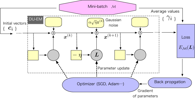
The optimization process is summarized in Algorithm 1. This optimization algorithm is mainly based on the Deep-unfolded Euler-Maruyama (DU-EM) method for approximating . The initial value of the matrix is assumed to be the zero matrix . The main loop can be regarded as a stochastic gradient descent method minimizing the loss values. The update of (line 5) can be done by any optimizer such as the Adam optimizer. The gradient of the loss function (line 4) can be easily evaluated by using an automatic differentiation mechanism included in recent neural network frameworks such as TensorFlow, PyTorch, Jax, and Flux.jl with Julia. The block diagram of the Algorithm 1 is shown in Fig. 4.
The stochastic optimization process outlined in Algorithm 1 is unable to guarantee that the obtained solution will be strictly feasible. To ensure feasibility, it is necessary to search for a feasible solution that is near the result obtained by optimization. This is accomplished by using the round function at line 7 of Algorithm 1.
The specific details for the round function used for optimization problem A are outlined in Algorithm 2. The first step in the algorithm, , ensures that the resulting matrix is symmetric. The nested loop from line 2 to line 7 is used to enforce the degree constraint and the constraint . The single loop from line 9 to line 11 is implemented to satisfy the constraint . The output of the round function guarantees that the constraints (67)-(70) of optimization problem A are strictly satisfied. A similar round function can be constructed for optimization problem B, which is presented in Algorithm 3.
VI Numerical results
VI-A Choice of Number of bins for EM-method
In the previous sections, we proposed a DU-based optimization method. This section presents results of numerical experiments. For these experiments, we used the automatic differentiation mechanism provided by Flux.jl [25] on Julia Language [26].
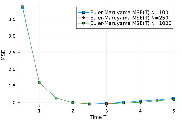
Before discussing the optimization of MSE, we first examine the choice number of bins, . Small is beneficial for computational efficiency but it may lead to inaccurate estimation of MSE. In this subsection, we will compare the Monte carlo estimates of MSE estimated by the EM-method.
The Karate graph is a well-known graph of a small social network. It represents the relationships between 34 members of a karate club at a university. The graph consists of 34 nodes, which represent the members of the club, and 78 edges, which represent the relationships between the members.
Figure 5 compares three cases, i.e., . No visible difference can be observed in the range from to . In the following experiments, we will use for EM-method.
VI-B Petersen graph (Optimization problem A)
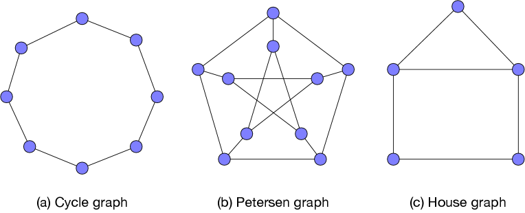
Petersen graph is a 3-regular graph with nodes (Fig.6(a)). In this subsection, we will examine the behavior of our optimization algorithm of for Petersen graph.
An adjacency matrix of a graph is defined by
| (88) |
An unweighted Laplacian matrix is defined by
| (89) |
The degree matrix is a diagonal matrix where is the degree of the node . Namely, an unweighted Laplacian corresponds the case where for any .
In the following discussion, let be the unweighted Laplacian matrix of Petersen graph. We assume Optimization problem A with the degree sequence .
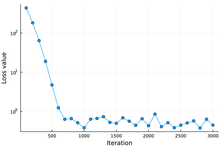
The parameter setting is as follows. The mini-batch size is set to . The noise intensity is . The penalty coefficients are . For time discretization, we use . The number of iterations for an optimization process is set to 3000. The tolerance parameter is set to . In the optimization process, we used the Adam optimizer with a learning rate of 0.01.
The loss values of an optimization process of Algorithm 1 are presented in Fig.7. In the initial stages of the optimization process, the loss value is relatively high since the initial is set to the zero matrix, which means that the system cannot achieve average consensus. The loss value decreases monotonically until around iteration 700, after which it fluctuates within a range of . The graph shows that the matrix in Algorithm 1 is being updated appropriately and that the loss value, which approximates , is decreasing.
Let us denote the Laplacian matrix obtained by the optimization process as . Table I summarizes several important quantities regarding . The top 4 rows of Table I indicate that is certainly a feasible solution satisfying (67)–(70) because we set . This numerical results confirms that the round function works appropriately. The last row of Table I shows that is very close to the unweighted Laplacian matrix . Since Petersen graph is regular and has high symmetry, it is conjectured that is the optimal solution for Optimization problem A. Thus, the closeness between and can be seen as a convincing result.
| 0 | |
| 0 | |
| 0 | |
| 0.188 |
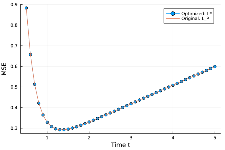
The MSE values of the optimization result and the unweighted Laplacian matrix are presented in Fig.8. These values are evaluated by the MSE formula (64). No visible difference can be seen between two curves. This means that Algorithm 1 successfully found a good solution for Optimization problem A in this case.
VI-C Karate graph (Optimization problem A)
We here consider Optimization problem A on the Karate graph. Let be the unweighted Laplacian matrix of the Karate graph. The target degree sequence is set to The parameter setting for an optimization process is given as follows. The mini-batch size is set to . The noise intensity is set to . The penalty coefficients are . We use for DU-EM method. The number of iterations for an optimization process is set to 5000. The tolerance is set to . In the optimization process, we used the Adam optimizer with learning rate 0.01.
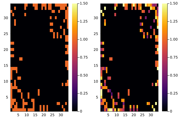
Assume that is the Laplacian matrix obtained by an optimization process. The matrix is a feasible solution satisfying all the constraints (67)–(70). For example, we have . Figure 9 presents the absolute values of non-diagonal elements in and . According to its definition, the absolute value of a non-diagonal element of take the value one (left panel). On the other hand, we can observe that non-diagonal elements of takes the absolute values in the range to .
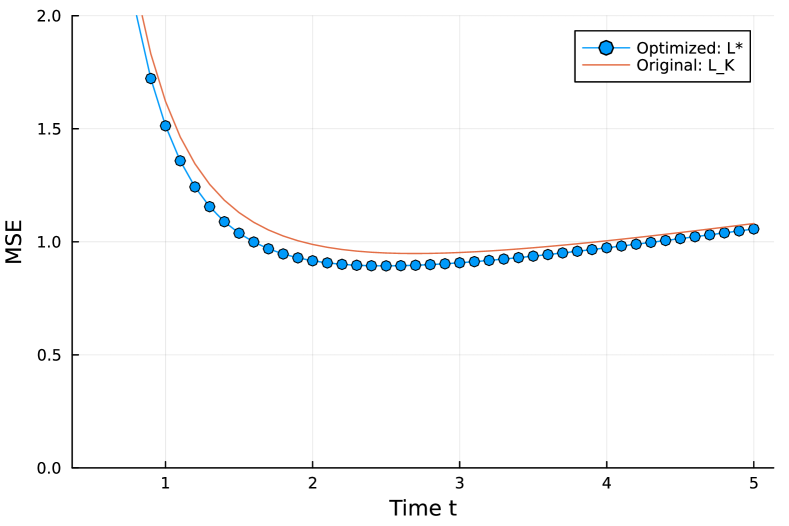
We present the MSE values of the optimization result and the unweighted Laplacian matrix in Fig.10. These values are evaluated by the MSE formula (64). It can be seen that the optimized Laplacian provides smaller MSE values. In this case, appropriate assignment of weights improves the noise immunity of the system. The inverse eigenvalue sums of the Laplacian matrices and are 13.83 and 13.41, respectively. In this case, the optimization process of Algorithm 1 can successfully provide a feasible Laplacian matrix with smaller inverse eigenvalue sum. As shown in (65), the inverse eigenvalue sum determines the behavior of .
VI-D House graph (Optimization problem B)
The house graph (Fig.6(c)) is a small irregular graph with 5 nodes defined by the adjacency matrix:
| (90) |
We thus have the unweighted Laplacian of the house graph as
| (91) |
where the diagonal sum of is 12.
We made two optimizations for and . The parameter setting is almost the same as the one used in the previous subsection. Only the difference is to use as the diagonal sum penalty constant. As results of the optimization processes, we have two Laplacian matrices and as follows:
| (92) |
| (93) |
The diagonal sums of and are 12.04 and 23.99, respectively. Compared with with , the diagonal elements of are more flat:
| (94) | ||||
| (95) |
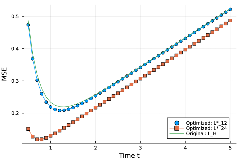
The MSE values of the optimization result and the unweighted Laplacian matrix are shown in Fig.11. We can observe that achieves slightly smaller MSE values compared with the unweighted Laplacian matrix . The Laplacian matrix provides much smaller MSE values than those of . The sums of inverse eigenvalues are for , , and , respectively.
VI-E Barabási-Albert (BA) random graphs (Optimization problem B)
As an example of random scale-free networks, we here handle Barabási-Albert random graph which use a preferential attachment mechanism. The number of edges between a new node to existing nodes is assumed to be 5.
In this experiment, we generated an instance of Barabási-Albert random graph with 50 nodes. The unweighted Laplacian of the instance is denoted by . The sum of the diagonal elements of is . The parameter setting for optimization is the same as the one used in the previous subsection except for . The output of the optimization algorithm is referred to as .
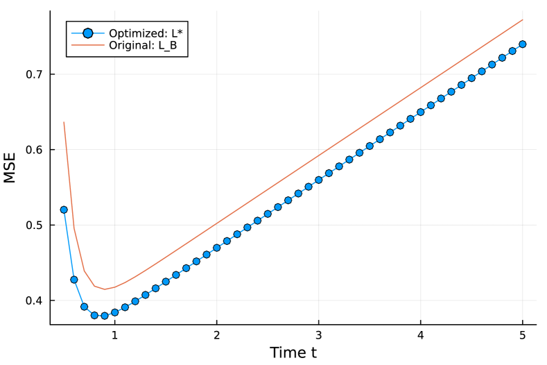
Figure 12 presents the MSE values of the original unweighted Laplacian and the optimization output . We can observe that the optimized MSE values are substantially smaller than those of the unweighted Laplacian . The sums of inverse eigenvalues for and are and , respectively.
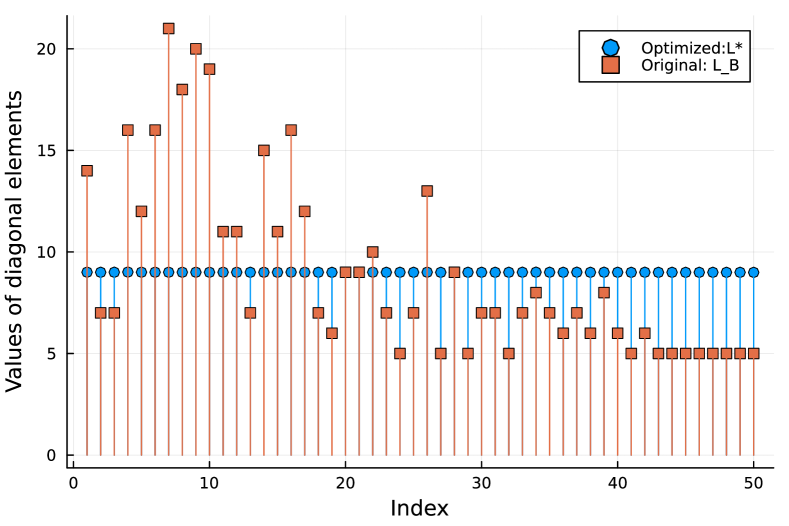
Figure 13 illustrates the values of diagonal elements of and . It can be observed that the values distribution of is almost flat although the values of varies from 5 to 21. This observation is consistent with the tendency observed in the previous subsection regarding the house graph.
VII Conclusion
In this paper, we have formulated a noisy average consensus system through a SDE. This formulation allows for an analytical study of the stochastic dynamics of the system. We derived a formula for the evolution of covariance for the EM method. Through the weak convergence property, we have established Theorem 1 and derived a MSE formula that provides the MSE at time . Analysis of the MSE formula reveals that the sum of inverse eigenvalues for the Laplacian matrix is the most significant factor impacting the MSE dynamics. To optimize the edge weights, a deep unfolding-based technique is presented. The quality of the solution has been validated by numerical experiments.
It is important to note that the theoretical understanding gained in this study will also provide valuable perspective on consensus-based distributed algorithms in noisy environments. In addition, the methodology for optimization proposed in this paper is versatile and can be adapted for various algorithms operating on graphs. The exploration of potential applications will be an open area for further studies.
Acknowledgement
This study was supported by JSPS Grant-in-Aid for Scientific Research (A) Grant Number 22H00514. The authors thank Prof. Masaki Ogura for letting us know the related work [11] on discrete-time average consensus systems.
References
- [1] T. Wadayama and A. Nakai-Kasai, “Continuous-time noisy average consensus system as Gaussian multiple access channel,” IEEE International Symposium on Information Theory, (ISIT) 2022.
- [2] R. Olfati-Saber and R. M. Murray, “Consensus problems in networks of agents with switching topology and time-delays,” IEEE Trans. Automat. Contr., vol. 49, no. 9, pp. 1520–1533, Sept. 2004.
- [3] R. Olfati-Saber, J. A. Fax, and R. M. Murray, “Consensus and cooperation in networked multi-agent systems,” Proceedings of the IEEE, vol. 95, no. 1, pp. 215–233, 2007.
- [4] W. Reb and R. W. Beard, “Consensus seeking in multi-agent systems under dynamically changing interaction topologies,” IEEE Transactions on Automatic Control, vol. 50, no. 5, pp. 655–661, 2005.
- [5] L. Xiao and S. Boyd, “Fast linear iterations for distributed averaging,” Systems and Control Letters, vol. 53, pp. 65–78, 2004.
- [6] W. Ren, “Consensus strategies for cooperative control of vehicle formations,” IET Control Theory and Applications, vol.2, pp. 505–512, 2007.
- [7] P. E. Kloeden and E. Platen, “Numerical solution of stochastic differential equations,” Springer-Verlag, 1991.
- [8] B. Oksendal, “Stochastic differential equations: an introduction with applications,” Springer, 2010.
- [9] C. Godsil and G. F. Royle, “Algebraic graph theory,” Springer, 2001.
- [10] F. Chung, “Spectral graph theory,” American Mathematical Society, 1997.
- [11] A. Jadbabaie and A. Olshevsky, “On performance of consensus protocols subject to noise: Role of hitting times and network structure,” IEEE 55th Conference on Decision and Control (CDC), pp. 179-184, 2016.
- [12] R. Rajagopal and M. J. Wainwright, “Network-based consensus averaging with general noisy channels,” IEEE Trans. Signal Process., vol. 59, no. 1, pp. 373–385, Jan. 2011.
- [13] M. Kishida, M. Ogura, Y. Yoshida, and T. Wadayama, “Deep learning-based average consensus,” IEEE Access, vol. 8, pp. 142404 - 142412, 2020.
- [14] B. Aazhang, B. P. Paris and G. C. Orsak, “Neural networks for multiuser detection in code-division multiple-access communications,” IEEE Trans. Comm., vol. 40, no. 7, pp. 1212-1222, Jul. 1992.
- [15] E. Nachmani, Y. Beéry and D. Burshtein, “Learning to decode linear codes using deep learning,” 2016 54th Annual Allerton Conf. Comm., Control, and Computing, 2016, pp. 341-346.
- [16] T. O’Shea and J. Hoydis, “An introduction to deep learning for the physical layer,” IEEE Trans. Cog. Comm. Net., vol. 3, no. 4, pp. 563-575, Dec. 2017.
- [17] Y. A. LeCun, L. Bottou, G. B. Orr, and K. R. Müller, “Efficient backprop,” in Neural networks: Tricks of the trade, G. B. Orr and K. R. Müller, Eds. Springer-Verlag, London, UK, 1998, pp. 9-50.
- [18] D. E. Rumelhart, G. E. Hinton, and R. J. Williams, “Learning representations by back-propagating errors,” Nature, vol. 323, no. 6088, pp. 533-536, Oct. 1986.
- [19] M. Borgerding and P. Schniter, “Onsager-corrected deep learning for sparse linear inverse problems,” 2016 IEEE Global Conf. Signal and Inf. Process. (GlobalSIP), Washington, DC, Dec. 2016, pp. 227-231.
- [20] M. Borgerding, P. Schniter, and S. Rangan, “AMP-inspired deep networks for sparse linear inverse problems, ” IEEE Trans, Sig. Process. vol 65, no. 16, pp. 4293-4308 Aug. 2017.
- [21] K. Gregor, and Y. LeCun, “Learning fast approximations of sparse coding,” Proc. 27th Int. Conf. Machine Learning, pp. 399-406, 2010.
- [22] A. Balatsoukas-Stimming and C. Studer, “Deep Unfolding for Communications Systems: A Survey and Some New Directions,” 2019 IEEE International Workshop on Signal Processing Systems (SiPS), pp. 266-271, 2019.
- [23] D. Ito, S. Takabe, and T. Wadayama, ”Trainable ISTA for sparse signal recovery,” IEEE Transactions on Signal Processing, vol. 67, no. 12, pp. 3113-3125, 2019.
- [24] C. Rackauckas, Y. Ma, J. Martensen, C. Warner, K. Zubov, R. Supekar, D. Skinner, A. Ramadhan, and A. Edelman, “Universal differential equations for scientific machine learning,” arXiv:2001.04385, 2020.
- [25] M. Innes, “Flux: Elegant machine learning with Julia,” Journal of Open Source Software, 2018.
- [26] J. Bezanson, S. Karpinski, B. Viral, and A. Edelman, “Julia: A fast dynamic language for technical computing,” arXiv preprint arXiv:1209.5145, 2012.
- [27] R. Albert, A.-L. Barabasi, “Statistical mechanics of complex networks,” American Physical Society, Rev. Mod. Phys., vol.74 pp. 47–97, 2002.