Stochastic estimation of Green’s functions with application to diffusion and advection-diffusion-reaction problems
Abstract
A stochastic method is described for estimating Green’s functions (GF’s), appropriate to linear advection-diffusion-reaction transport problems, evolving in arbitrary geometries. By allowing straightforward construction of approximate, though high-accuracy GF’s, within any geometry, the technique solves the central challenge in obtaining Green’s function solutions. In contrast to Monte Carlo solutions of individual transport problems, subject to specific sets of conditions and forcing, the proposed technique produces approximate GF’s that can be used: a) to obtain (infinite) sets of solutions, subject to any combination of (random and deterministic) boundary, initial, and internal forcing, b) as high fidelity direct models in inverse problems, and c) as high quality process models in thermal and mass transport design, optimization, and process control problems. The technique exploits an equivalence between the adjoint problem governing the transport problem Green’s function, and the backward Kolmogorov problem governing the transition density, of the stochastic process used in Green’s function construction. We address nonspecialists and report four contributions. First, a recipe is outlined for diagnosing when stochastic Green’s function estimation can be used, and for subsequently estimating the transition density and associated Green’s function. Second, a naive estimator for the transition density is proposed and tested. Third, Green’s function estimation error produced by random walker absorption at Dirichlet boundaries is suppressed using a simple random walker splitting technique. Last, spatial discontinuity in estimated GF’s, produced by the naive estimator, is suppressed using a simple area averaging method. The paper provides guidance on choosing key numerical parameters, and the technique is tested against two simple unsteady, linear heat conduction problems, and an unsteady groundwater dispersion problem, each having known, exact GF’s.
keywords:
stochastic estimation of Green’s functions , linear and nonlinear transportPACS:
0000 , 1111MSC:
0000 , 1111[inst1]organization=Department of Mechanical Engineering and Engineering Science,addressline=9201 University City Blvd., city=Charlotte, postcode=28223, state=North Carolina, country=United States
[inst2]organization=University of Tennessee Space Institute, city=Huntsville, postcode=35649, state=Alabama, country=United States
[inst3]organization=Department of Physics and Optical Science,addressline=9201 University City Blvd., city=Charlotte, postcode=28223, state=North Carolina, country=United States
1 Introduction
Considering a physical system whose dynamics are determined by a set of conservation laws and physical principles, finding a Green’s function that reliably models the system’s spatial and temporal response to forcing opens the door to a number of powerful capabilities. Focusing on thermal and chemical transport in complicated, irregular regions, the temporal thermal or chemical response at discrete locations, to an infinite array of space and time-dependent forcing, for example, can be readily determined [1, 2]. Similarly, Green’s functions can be incorporated in inverse problems, allowing, for example, extraction of thermal and pollutant source locations and strengths, based on limited temperature and chemical measurements; see references and examples in [3, 4, 5]. Green’s functions can also provide a basis for efficient thermal and mass transport design, optimization, and process control [6, 7, 8]. In these applications, a reliable Green’s function can replace approximate or empirical system models, improving the reliability and quality of a design or control process.
Unfortunately, building a Green’s function rests on three typically challenging tasks:
A) derive (or, when possible, look up) the adjoint equation governing the Green’s function (GF);
B) simultaneously derive the integral solution for the evolving field variable, - which we’ll call the ’magic rule’ [2] - stated in terms of convolutions of the Green’s function with initial and boundary conditions, as well as in-domain forcing terms, and
C) find an appropriate Green’s function, subject to the governing adjoint problem derived in steps A) and B).
Most texts treating Green’s function techniques do not illustrate the trial and error nature of the first two steps, leaving non-specialists with limited insight. We address this deficiency in Appendix C, simultaneously deriving, via trial and error, the adjoint equation and magic rule associated with a linear advection-diffusion problem.
Importantly, most of the difficulty surrounding Green’s function solutions is tied to task C). A number of texts illustrate this step, invariably focusing on solution of (given, non-derived) adjoint equations, stated in simple geometries, leading to analytical Green’s function solutions [1, 2, 9]. For linear transport problems in complex geometries, however, this step clearly requires a numerical attack. Unfortunately, little work has been reported on numerical construction of Green’s function’s, specifically, numerical solution of adjoint equations associated with transport problem-specific partial differential equations, such as Eqs. (1) and (2) below. While boundary element (BEM) [10, 11, 12], Green element (GEM) [13, 14, 15], and finite element methods (FEM) [16, 17, 18, 19] are widely characterized as Green’s function techniques, none of these explicitly solve problem-specific adjoint equations. As a consequence, these only allow whole-domain solutions, in contrast to the pointwise solutions obtained by the technique proposed here.
We focus on construction of approximate GF’s, appropriate to solution of advection-diffusion-reaction problems of the general form:
| (1) |
subject to specified boundary and initial conditions. Here, is a scalar field property (often a density of some kind), subject to: i) transport by diffusion/dispersion real-valued ) and/or ii) wave propagation complex-valued), iii) advective transport by a fluid velocity field, iv) depletion by first order chemical reaction, and v) augmentation or depletion by a source/sink field, In addition, represents an anisotropic, often position- and time-dependent diffusion or dispersion tensor, is a solute-dependent chemical or radiological decay constant, where and have no dependence on while is at most, linearly dependent on Importantly, the dispersion/diffusivity, velocity and source/sink fields are known quantities.
In situations where the dispersion/diffusion tensor, is diagonal - capturing diffusive or dispersive transport that’s dominant in one, two, or three mutually orthogonal directions, the substitutions and , can be used to transform Eq. (1) into an equation of the form,
| (2) |
As discussed in the third validation test below, equations of the form (1) arise, for example, in models of solute transport in aquifers [20]. Equation (2) appears in many areas of physics, biology, and engineering, including fluid mechanics (linearized Navier-Stokes equations) [21, 22], drift-diffusion [23] and reaction-diffusion problems [24, 25]), quantum mechanics (Schrödinger equation) [26], statistical mechanics (Fokker-Planck equation) [27] and plasma physics (Vlasov equation) [28]. Wave equations [29, 30] and Chapman-Kolmogorov equations [31] can also be expressed in this form.
Since ’backward time’ stochastic construction of GF’s provides the single-point response at a chosen ’response point’, as produced by any given set of boundary and initial conditions, we focus most of the discussion on backward time Green’s function construction. For testing and validation purposes, however, the last validation case uses forward time stochastic construction. As discussed in test 3, forward time construction: i) can be used when the diffusion/dispersion tensor is diagnonal: where is a tensor function of position and time, and is the identity matrix, and ii) provides the response at as produced by an impulse at a specific ’impulse point’,
Focusing on backward time construction, the proposed approach launches a swarm of RW’s backward in time from a chosen response point, calculating the random, backward trajectories of each random walker, using a transport-problem-specific stochastic differential equation. The transition (probability) density, for observing the random walker at a chosen ’impulse point’, given that it started at is then estimated. Under conditions where the transport problem’s adjoint problem - governing evolution of the propagator, - has the same structure as the so-called backward Kolmogorov problem - governing evolution of - the estimated transition density allows estimation of the propagator, and in turn, the Green’s function.
In overview, we first outline a step-by-step recipe for stochastically constructing GF’s, appropriate to transport problems governed by Eqs. (1) and (2). The proposed stochastic Green’s function estimation technique is then contrasted against Monte Carlo approaches for (approximately) solving initial-boundary value problems (IBVP’s) [32, 33, 34, 35, 36, 37]: The former bypasses complicated, often impossible derivation of stochastic representative solutions required for the latter, and, in addition, provides an approximate input-response (GF) function, applicable to generic IBVP’s, subject to any combination of Dirichlet, Neumann, and/or Robin BC’s. A simple naive estimator [38, 39, 40, 41, 42] for the transition density, is then derived and heuristically validated using a central limit argument. Numerical validation tests reveal two significant sources of error: depletion of the initial random walker swarm due to absorption at Dirichlet boundaries, and spatial discontinuity in estimated Green’s function’s, produced by our naive density estimator. To solve the first problem, we propose a simple particle splitting technique which preserves the number of simulated random walker’s launched, as well as satisfying continuum mass conservation at the splitting point. A simple area-averaging technique is proposed for tackling the second problem. In order to stochastically estimate GF’s, three numerical parameters must be chosen: the number of random walker’s launched, from a chosen response point, the interrogation area, on which random walker’s are captured, and the time step, used for estimating random walker trajectories. Strategies for choosing these parameters are outlined in S1 Appendix A. Finally, the Green’s function estimation technique is tested against three test problems, of increasing complexity, each having known GF’s.
2 Recipe: Stochastic estimation of Green’s functions
Using stochastic methods to estimate GF’s requires a number of analytical and numerical steps. In order to provide an overview of the proposed technique, we outline the steps here.
Step 1: Simultaneously determine the adjoint problem governing the Green’s function and the magic rule: Using Green’s identities, and by trial and error, simultaneously determine the adjoint equation, the magic rule [1, 2], and the boundary and initial conditions on the adjoint equation. We illustrate this step in Appendix C, using a simplified, constant coefficient advection-diffusion problem.
Step 2: Postulate that continuum transport reflects microscale stochastic dynamics: This step provides a physical connection between microscale and continuum transport, as well as the mathematical basis for Steps 4 and 5. Express as a functional, of a Brownian stochastic process, [31, 43, 44],
| (3) |
evolving in backward time, according to
| (4) |
where is an n-dimensional Weiner process, is the reversed drift/velocity field, and where the diffusion matrix is tied to by
| (5) |
with the average representing the conditional expectation In addition, the relationships between backward and forward (actual) time instants are as follows: i) the chosen, fixed (actual) response time, corresponds to the fixed backward instant, from which the random walker swarm is launched: ii) the variable (actual) impulse time, corresponds to the variable backward random walker capture time, iii) the magnitude of forward time difference, equals the backward time difference,
Step 3: Determine the backward Kolmogorov problem governing backward evolution of the transition density: The probability of observing a backward moving random walker, governed by (4), at given that it started at is given by the probability density function, As discussed in Step 4, the present step is required in order to ensure that the adjoint problem governing the Green’s function coincides with the terminal-boundary value problem governing
The backward time evolution of is governed by the backward Kolmogorov equation [31, 43, 44]:
| (6) |
where is subject to the terminal backward time condition:
| (7) |
Boundary conditions on (6) that are relevant to, and correspond respectively to Dirichlet, Neumann, and Robin BC’s in typical advection-diffusion-reaction problems, are as follows [43, 44]:
| (8) |
| (9) |
and
| (10) |
In Eq. (8), denotes the space-time boundary on which Dirichlet BC’s are imposed on the physical transport problem. Similar definitions for Neumann and Robin boundaries are given respectively in (9) and (10). The conormal vector is defined as [44] where is the local unit outward normal. Finally, in mass transfer problems, is the local reaction coefficient [44], arising, for example, on reactive boundaries. In heat transfer problems, corresponds to the local convective heat transfer coefficient, divided by the local thermal conductivity.
Step 4: Determine the applicability of the Green’s function estimation method: For transport problems in which diffusive or dispersive transport is non-negligible, stochastic estimation of GF’s can only be used if the adjoint problem governing the so-called propagator, coincides with the backward Kolmogorov problem, governed by Eq. (6) and problem-specific combinations of the BC’s in Eqs. (8) through (10). Specifically:
a) the diffusion/dispersion matrix must be diagonal:
| (11) |
This requirement emerges in Step 1: Non-diagonal produces a convolution integral, over the problem domain, in two unknowns, the Green’s function and
b) The spatial domain, in which transport takes place, must remain fixed/non-deforming; this ensures that time-invariance and symmetry properties intrinsic to the propagator are enforced [2].
Under conditions a) and b), the problem governing the propagator, mirrors the problem governing with replacing in Eqs. (6) through (10). Given an estimated propagator, the associated Green’s function is then given by [2]:
| (12) |
where is the Heaviside function.
Step 5: Choose a scheme for integrating Eq. (4) and an estimator for estimating Various approaches, each characterized by a pointwise (strong) order of convergence, are available for numerically integrating stochastic differential equations, here Eq. (4) [45, 46, 47, 48]. Since boundary conditions on the adjoint equation are all-determining in constructing the Green’s function, and since interaction of stochastic processes with Dirichlet, Neumann, and Robin boundaries, as integrated by the Euler-Maruyama scheme [45, 47, 49] have been well-studied [44], this scheme is recommended. We note below, however, alternative, less expensive integration schemes.
3 Comparison of proposed Green’s function estimation method with Monte Carlo solutions of initial-boundary value problem; limitations
Monte Carlo (MC) techniques for solving linear partial differential equations, subject to problem-specific boundary and initial conditions, have a long history [50, 51, 52]. By contrast, stochastic construction of GF’s via transition density estimation appears to represent a new and more general approach, where the estimated Green’s function can be used to (approximately) solve a given linear PDE, subject to any combination of initial and boundary conditions. In order to contrast the proposed stochastic Green’s function estimation method against MC solutions of IBVP’s [32, 33, 34, 35, 36, 53], we outline the five-step construction of MC solutions, and then touch on the significant differences and advantages introduced by the present approach.
Monte Carlo solutions are based on representative stochastic solutions of elliptic, parabolic, and hyperbolic PDE’s, subject to specific boundary conditions, and in the latter two cases, initial conditions [54, 55, 56, 57, 58]. Focusing on parabolic problems governed, for example, by Eqs. (1) or (2), the recipe is as follows: i) Assume that macroscopic evolution of the field variable, reflects (long time scale, collective [21, 44]) microscale advective-diffusive transport of some conserved real or virtual property, e.g., microscopic number, momentum, or energy density [21, 59, 60], represented by and modeled by Eq. (4). ii) Using Ito’s formula [31, 43, 44], determine the differential, backward-time change in produced by the stochastic evolution of iii) In the equation derived in step ii), and referring to (1), replace the temporal derivative of along with advective and diffusive terms with remaining source and reaction terms, and respectively. iv) Attempt to obtain a stochastic representative solution for by integrating, backward in time, the differential equation obtained in iii). In deriving the representative solution, account for the stochastic process sampling Dirichlet, Neumann, and/or Robin boundaries that appear in the continuum transport problem [55, 56, 57, 58]. v) Using the representative solution obtained in step iv), launch a random walker swarm from a chosen solution point, and use appropriate absorption (Dirichlet boundaries), reflection (Neumann boundaries), and partial reflection (Robin boundaries) techniques [44] to construct a Monte Carlo estimate for
Comparing the MC approach with the proposed Green’s function estimation procedure, two significant advantages emerge. First, by directly estimating transition densities Green’s function estimation bypasses the challenging task of deriving representative stochastic solutions [55, 56, 57, 58]: Steps iii) and iv) are eliminated in favor of straightforward stochastic integration of Eq. (4), combined with well-developed boundary interaction techniques [44]. Second, as noted above, the technique produces an estimated, non-problem-specific input-response function (Green’s function) that can be used to solve a family of advection-diffusion-reaction problems, subject to any combination of Dirichlet, Neumann, and/or Robin BC’s.
3.1 Challenges and a limitation
The present work is experimental, focused on developing a stochastically-based Green’s function estimation technique. Prior to looking at details, we highlight two significant challenges that required solution, and note a limitation associated with the method in its current form.
First, following launch of a random walker swarm - consisting of integrated realizations of Eq. (4) - from a chosen solution point, absorption of individual realizations at Dirichlet boundaries rapidly depletes the initial set of random walkers. Depletion, in turn, produces increasingly degraded-in-time Green’s function estimates. Our solution, based on respawning of weighted random walker’s, and carried out at random locations in the problem domain, enforces continuum conservation of mass at the particle respawning point, and significantly improves Green’s function estimation accuracy. See Section 6.3. Second, spatial variance in estimated GF’s likely arises due to use of a spatially discontinuous naive density estimator [38, 40], Eq. (13) below. We address this problem by introducing an area-averaging technique in which variance in local Green’s function estimates is minimized by iteratively altering the size of a smoothing window. See Section 6.4. Although not investigated, kernel estimators, which also eliminate discontinuity in naive estimators [38, 40], might also prove advantageous.
Regarding the present technique’s main limitation, Euler-Murayama integration of Eq. (4) has a low order of strong convergence [45, 46, 47]. For a given degree of Green’s function estimation accuracy, significantly faster integration can be achieved using, for example, Milstein’s order 1 method [46], or order 2 strong Taylor expansion methods [47], or order 2 Runge-Kutta methods [48]. However, again, since boundary conditions on the adjoint problem are central to constructing the estimated Green’s function, and since treatment of random walker-boundary interactions has reached maturity in the case of Euler-Murayama integration [44], this scheme is used.
4 A simple estimator for the transition density
Transition density estimation remains a research-level task [38, 39, 40, 41, 42]. An accessible overview of theoretical results, focused on the simplest case of estimating ’free-space’ transition densities, can be found in [39].
In this study, the transition density is estimated using the naive estimator [38]:
| (13) |
where, the estimation error is determined by the Euler-Murayama scheme’s weak convergence order [31, 46, 47], and where and are, respectively, the number of RW’s launched from the solution point, the chosen RW interrogation area, centered on at backward time, and the number of RW’s that reach or pass through over the time interval,
While the formula in Eq. (13) is stated in terms of the Lebesque measure in, e.g., [40], it can be derived heuristically as follows. Focus on two-dimensional random walks, as used in our tests, evolving within an arbitrary two-dimensional domain, subject to any combination of Dirichlet, Neumann and/or Robin boundaries. For two-dimensional problems, it is useful to picture a three-dimensional, cylindrical hyperspace in which the downward (upward) vertical direction corresponds to the backward (forward) time axis, the top corresponds to the backward (forward) solution time slice, the bottom to the backward (forward) terminal (initial) time slice, with any horizontal slice through the hyperspace corresponding to an instantaneous snapshot of the two-dimensional spatial domain,
Symbolically, recognize that the probability of random walker’s, launched from reaching a chosen interrogation area, at the instant is given by:
| (14) |
Assuming that is well-behaved, then in the limit as by the mean-value theorem,
| (15) |
where and as
Thus, based on the numerical simulation of random walker evolution following launch, approximate the probability on the left side of Eq. (14) as
| (16) |
Combining Eqs. (14) through (16) then leads to the estimator in (13). As highlighted in [38], and as we find below, estimators like Eq. (13) produce discontinuous estimates of
4.1 Heuristic validation of estimator, Eq. (13)
We adapt a central limit argument in [61] to estimate the free-space transition density, for the evolution of a numerically simulated swarm of RW’s, launched from within an infinite, two-dimensional domain. Of the RW’s launched, focus on the RW’s that reach or pass through differential area, over the backward time interval, where and
Define the space-time vector displacement of the random walker, in the set of RW’s captured by as
| (17) |
or, in component form,
| (18) |
where
| (19) |
is the simulated Brownian displacement of random walker over the time-interval.
Now, let so that, likewise, and define the random variable as the sum of independent random variables,
| (20) |
where is the sum of variances of the set of differential x-displacements. Importantly, recognize that the differential spread, i.e., variance, in backward time x-displacements (over the set of random walker trajectories captured on decreases with increasing backward time: or, in terms of forward time increments,
Letting so that then by the central limit theorem [61], the probability density for tends to the Gaussian:
| (21) |
where, since The same argument applied to the y-component of the random relative displacement, leads to:
| (22) |
where again, and
Finally, letting then and Thus, we find that the simple estimator in Eq. (13) for the probability of observing a random walker at given that it was launched at given by the product of the right sides of Eqs. (21) and (22), corresponds to the solution of the diffusive backward Kolmogorov equation, Eq. (6):
| (23) |
Equivalently, and as required [31, 44], this corresponds to the free-space solution to the (pure diffusion) Fokker-Planck equation, governing forward time evolution of following delta function release of RW’s, at from
4.2 Green’s function estimate and error in the estimate
Assuming that the adjoint problem governing the propagator, and the backward Kolmogorov problem governing the transition density have the same structure, then from Eq. (12), for the stochastically estimated Green’s function follows immediately from Eq. (13):
| (24) |
where the Euler-Murayama scheme’s weak convergence is again highlighted.
We note that an additional, localized, error arises in connection with the random walker respawning algorithm introduced below. As shown in Appendix B, this is an implicit discretization error, confined to random locations in the solution domain where individual RW’s are respawned following absorption on Dirichlet boundaries.
5 Absorbing boundaries and random walker respawning
In order to mitigate against loss of absorbed RW’s and preserve early-forward-time solution accuracy, we introduce a random walker respawning algorithm [62], and discuss below and in Appendix B its properties:
a) Initially, at the chosen backward solution instant, the group of RW’s to be launched from the solution point, are all assigned a weight of 1, and each random walker weight is stored in an array, [62].
b) After every backward time-step, any random walker that reaches a Dirichlet boundary is removed, and the in-domain random walker, having the highest weight, in is also removed and replaced by two RW’s, each having weights equal to The replacement pair are placed at the same location occupied by
c) After each set of time-steps, the array is reordered, in descending order, according to the current set of random walker weights. Thus, high-mass RW’s that experience relatively few absorption events, in particular, those far from Dirichlet boundaries, tend towards Dirichlet boundaries over backward time, suppressing numerical thinning of near-boundary mass distributions.
When using the respawning algorithm, equation (24) must be modified:
| (25) |
where is the total weight (sum of weights) of the RW’s that reach .
5.1 Properties of the respawning algorithm
Appendix B shows that the respawning algorithm has two important properties which ensure the physical consistency of the algorithm, as well as a third that significantly enhances the statistical quality of the Green’s function estimation procedure:
a) The algorithm enforces, at each random respawning location, the continuum diffusion equation governing continuum random walker evolution.
b) Since the algorithm diffusively smooths, on short, single-time-step time-scales, instantaneous, localized mass gradients produced by respawning, the algorithm appears to be insensitive to the number of time steps, taken between reordering of the random walker weight array, In this first study, we have not performed tests to ascertain suitable ranges for in all cases,
c) Crucially, the respawning algorithm conserves the number of random walkers, initially launched. As shown in the Results below, preserving is essential to obtaining low-error Green’s function estimates.
6 Numerical experiments
We focus on three test cases, each of increasing complexity: 1) two-dimensional diffusive transport in a square, 2) diffusion in a circle, and 3) unsteady two-dimensional groundwater solute transport, produced by combined advection, dispersion, and chemical depletion in a nonhomogeneous, anisotropic, infinite region. We use the first test to expose and solve two principle challenges: a) loss of random walker’s at Dirichlet boundaries and b) spatial variance in estimated GF’s. The second test examines the performance of the Green’s function estimation procedure in domains having non-planar boundaries. Since tests 1 and 2 allow (preferred, optimal) backward time Green’s function construction, in the next section, we illustrate, in detail, the backward time Green’s function estimation recipe. The third test requires forward time Green’s function estimation; there, we briefly outline the corresponding recipe.
6.1 Application of the backward time Green’s function estimation recipe to pure diffusion test cases 1 and 2
6.1.1 Step 1: Simultaneously derive the adjoint equation and magic rule
Appendix C illustrates trial and error derivation of these two central relations, focusing on a generic advection-diffusion transport problem in a finite domain. Similar trial and error approaches were used to derive the adjoint equations and magic rules used in all three test cases. In tests 1 and 2, the adjoint equation is thus given by:
| (26) |
where is a fixed diffusion coefficient.
Considering the case where a combination of Dirichlet and Neumann boundary conditions are imposed, the magic rule assumes the form:
| (27) |
where and represent, respectively, the areal/volumetric source/sink term, boundary conditions on the Neumann and Dirichlet boundaries, and the initial condition. See Eq. (S1 Appendix C), Appendix C, with the advective (last) term turned off. In addition, is the local outward unit normal to the problem domain,
6.1.2 Steps 2 and 3: Postulate existence of a microscale stochastic transport process, and write down the associated backward Kolmogorov problem
Since test cases 1 and 2 model pure diffusion, the backward-time stochastic differential equation is obtained by dropping the drift term in Eq. (4):
| (28) |
where, from Eq. (5), Thus, the corresponding backward Kolmogorov equation, determined by dropping the drift term from Eq. (6), is given by
| (29) |
where satisfies the terminal condition in Eq. (7). Finally, in tests 1 and 2, Dirichlet boundary conditions, as stated in Eq. (8), are imposed at all points on both domain boundaries.
6.1.3 Step 4: Determine the applicability of the stochastic Green’s function estimation procedure
Comparing Eqs. (26) and (29), due to the non-zero right side in (26), it is clear that these do not have the same mathematical structure. However, the propagator, which is connected to the Green’s function, via Eq.(12), does satisfy the equation where Thus, using to operate on where using as well as the terminal condition, as we obtain Eq. (26).
Thus, since the problems governing the propagator, and transition density, have identical mathematical structure, including matching BC’s and IC’s, we can use a density estimation procedure to first estimate and then immediately obtain via Eq. (12).
6.1.4 Step 5: Choose an integration scheme for the problem SDE and a density estimation method
As noted, in all three tests, we use the Euler-Murayama scheme [44, 46, 47] to integrate Eq. (28). Thus, discretize the backward time axis as: where the chosen backward solution time, corresponds to a chosen forward solution time, is the chosen random walker interrogation time, and Defining as the psuedo-random, numerical approximation to the Weiner differential, in Eq. (28), the EM scheme is given by [44, 47]:
| (30) |
where the numerical approximation to the actual stochastic jump, in (28) is denoted as Details on simulation of can be found, for example, in [44, 47].
6.2 Explanatory notes
A) The stochastic estimation technique requires specification of three numerical parameters: i) the backward (forward) time-step size, ii) the interrogation area, and iii) the number of RW’s, launched from the chosen Green’s function solution point, Appendix A proposes procedures for specifying these parameters.
B) In all three tests, lengths, forward and backward times, and diffusion coefficients, are expressed in non-dimensional form: i) ii) , iii) where and are dimensional, problem-specific length and time-scales. In the first two tests, is a dimensional diffusion coefficient, and in the third, a dimensional dispersion coefficient. Throughout the rest of this paper, all functions, variables, and parameters without a tilde are dimensionless.
In all three tests, we choose a dimensionless solution time, and dimensionless length, In order to gain a sense of associated dimensional scales, consider diffusion of small molecular and ionic species in water, where since diffusive spread of a specie introduced at a point grows as then choosing time scales, equal to, e.g., and requires computational domains having dimensions on the order of and respectively. Similar considerations can be used in the groundwater transport problem in test 3.
C) In test 1, we discretize the square solution domain, having dimensionless length, into (square) interrogation areas. In test 2, a circular solution domain of dimensionless diameter, is inscribed and centered within the same unit square. Again, the square is discretized into square interrogation areas. Thus, in both tests, and where denotes the centroid of the interrogation area. While test 3 considers ground water transport in an infinite domain, for finite solution time, and under the groundwater flow conditions considered, we can again define a unit square solution domain, again having interrogation areas; see Section 7.
In tests 1 and 2, the dimensionless diffusion coefficient is specified as while in test 3, the dimensionless dispersion coefficient is also set as As described in test 1, after some trial and error, the backward time step is chosen as likewise, in test 3, Finally, in tests 1 and 2, the number of RW’s launched from a chosen (forward-time) response point, is in test 3, corresponding to the number of RW’s launched from a (forward-time) impulse point,
Based on these choices, and as detailed in Appendix A, the estimated relative spatial variation in captured RW’s, over the chosen forward solution interval, ranges between
where the maximum variation occurs at late forward (early backward) time, From Eq. (48) Appendix A, large, early-backward-time variations can be suppressed by choosing sufficiently large (or for forward time random walker integration, large enough Our choice for reflects a compromise between computational cost and variance reduction. In addition, our chosen are approximately five times the (average) incremental diffusion distance, thus, and consistent with the results below, we appear to be obtaining statistically reasonable estimates of
6.3 Test Case 1, Part A: Deleterious depletion of random walkers at Dirichlet boundaries, remediation via random walker respawning, and error due to overlarge time step size
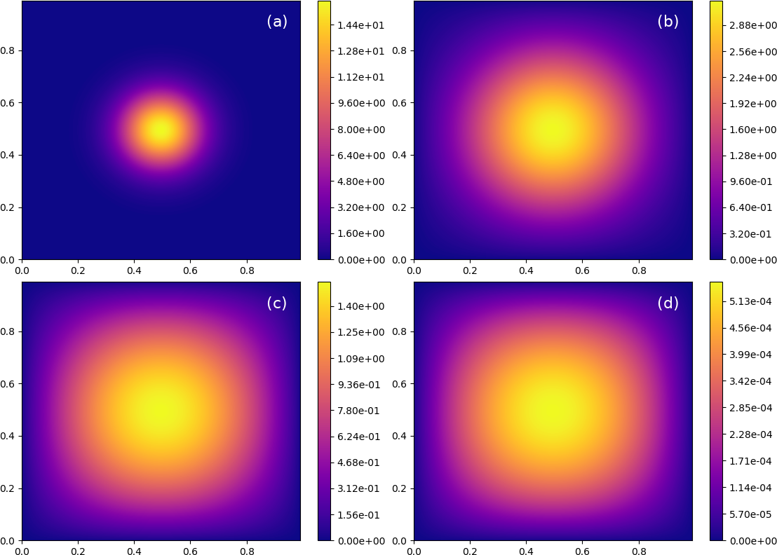
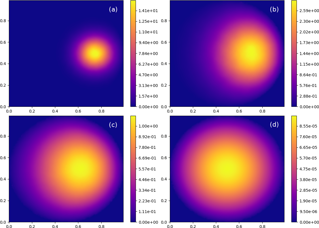
We use the first test case to emphasize the experimental nature of constructing Green’s function estimators, briefly highlighting the challenges we encountered, as well as our solutions. In test 1, the solution (response) point is chosen as In all figures, we show estimated and actual GF’s at various forward time instants, where For reference, Fig. 1 shows the exact Green’s function.
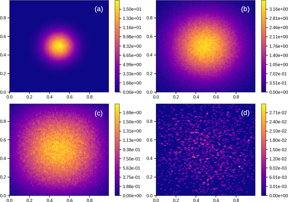
The detrimental effect of random walker absorption at Dirichlet boundaries is illustrated in Fig. 2, where depletion of RW’s becomes increasingly apparent as backward time integration of random walker trajectories proceeds. Comparing Figs. 1 and 2, we observe that the maximum local error,
| (31) |
increases from at forward time, to at Moreover, while relatively late forward time estimates, obtained at and shown respectively in Figs. 2a, 2b, and 2c, remain qualitatively consistent with the actual Green’s function in Fig. 1a-c, the early forward time estimate at Fig. 2d, is spatially amorphous, bearing no resemblance to the actual Green’s function depicted in Fig. 1d. While the results in Fig. 2 were obtained using a time step, which is approximately 2 orders of magnitude larger than the recommended , see Appendix A, similar qualitative results, not shown, are observed for
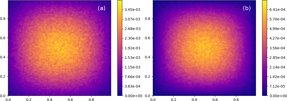
Introduction of random walker respawning significantly improves both the accuracy and the qualitative consistency of Green’s function estimates, as shown in Figs. 3a and 3b. These depict, respectively, at the early forward time, (corresponding to The two estimates shown in Figs. 3a and 3b use backward time steps, and respectively, which bracket the recommended Again, similar qualitative results are observed for
In order to improve the accuracy of the estimate shown in Fig. 3a, the too-large time step, is reduced to reducing the maximum relative error, again observed at from 570 % to 25 %. Although not shown, similar results are observed using
6.4 Test 1, Part B: Area averaging method for improving Green’s function estimation accuracy and smoothness
While reducing to magnitudes on the order of or less significantly improves Green’s function estimation accuracy, relative error, at long backward integration times, here, remains unacceptably large. Moreover, as shown in Fig. 3, plate b), long (backward) time estimated GF’s exihibit spatial graininess, an artifact of using the naive estimator in Eq. (25).
In order to address both issues, we introduce a simple area-averaging technique in which the value of in (25), obtained over an area, encompassing grid point is replaced with the average of all ’s observed at all grid points lying within a square , centered on Here, the smoothing window size, , is the smaller of two values: the distance to the nearest boundary, or a maximum window size, At any given backward time instant, is determined by iteratively altering in order to minimize the total root mean deviation,
| (32) |
between individual estimated and averaged Greens functions. Here, is the number of grid points included in the sum, is the estimated Green’s function at grid point , as given by (25), and is the averaged Green’s function. As noted, we use known, exact GF’s in place of The prime on the sum specifies that only those grid points where the summand is not equal to zero are included. We include this additional filter since, in many cases, there are a significant number of points in both the analytical and numerical Green’s function where both functions are zero. These flat areas, which can be seen in many late forward time GF’s, can skew the total deviation to spuriously low magnitudes.
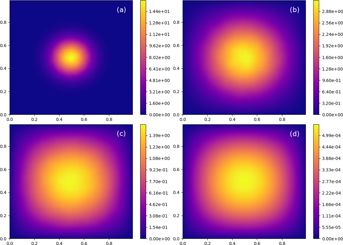
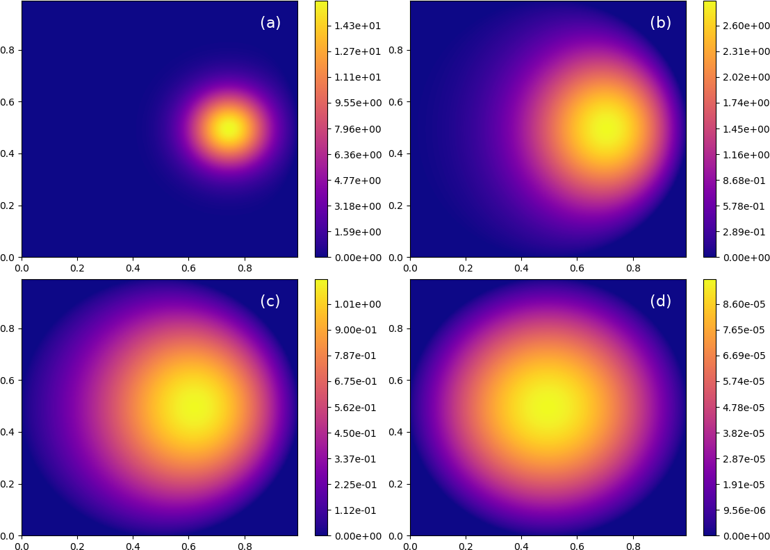
Finally, we observe that combining random walker respawning and area averaging provides relatively accurate estimated GF’s, as shown in Fig.4. Comparing estimated and exact GF’s, in Figs. 4 and 1, respectively, it is clear that, even at large backward estimation times, Fig. 4d, estimation accuracy and smoothness remain reasonable. At small backward estimation times, and shown respectively in Figs. 4a - c, maximum local relative errors remain less than and increase only to at in Fig. 4d. Note too that Green’s function magnitudes vary by more than five orders of magnitude over the chosen forward time interval, Although not tested here, but as indicated by the weak convergence of the Milstein-Euler integration scheme, we believe that improved accuracy can be obtained, at significantly higher computational cost, by further reductions in
Two final remarks are made concerning area averaging.
a) Beyond improved estimation accuracy and Green’s function smoothing, area averaging reduces the number of random walkers required to achieve a given level of accuracy, significantly improving computational efficiency. For example, experiments show that achieving late (backward) time accuracy, without area averaging, requires on the order of twenty million RW’s.
b) For poor Green’s function estimates, like those shown in Figure 3, plate a), no optimum window size can be found. There, the smoothing window minimizing the total deviation spans the entire domain, producing a constant function equal to the average of the values of all grid points.
6.5 Test 2: Green’s function estimates near curved boundaries
Many evolution problems take place in regions having complicated, non-planar boundaries. As a preliminary test of the stochastic Green’s function estimation procedure in such problems, we perform a second set of numerical experiments in which GF’s are constructed within a two-dimensional circular domain. Referring to Figures 6 and 5, a circular domain (boundary not shown), having radius 0.5 and center at , is inscribed and centered within the unit square shown. Here, any random walker that reaches or passes through the circle, is absorbed, triggering random walker respawning at a random location within the circle. For simplicity, the square is discretized into the same uniform set of square interrogation areas, used in test 1, introducing an discretization error in boundary-adjacent Green’s function estimates. As in Example 1, there is no flow , transport takes place by isotropic diffusion, with we use a backward-time step, and as in test 1, RW’s are launched, in this case, from a right-of-center solution point
In order to adapt the smoothing procedure to a circular domain, we define the smoothing window as a circle of radius centered on the grid point of interest. As before, is allowed to vary, being the smaller of two values: the distance to the boundary and the maximum window size. By this approach, the smoothing window is always contained within the circular domain. Although not explored here, beyond circular and square/rectangular smoothing window shapes - the former useful for domains having curved boundaries - polygonal shapes may also prove useful.
Exact and estimated GF’s are shown respectively in Figs. 5 and 6. In this case, and in contrast to test 1, the largest estimation errors are observed at the earliest backward time instant, Comparing patterns in maximum relative error evolution in test 1 and 2, Figs. 4 and 6, as expected, in test 1, progressively increases with increasing at least for and By contrast, in test 2, progressively decreases at all four probed time instants. These results indicate the following: I) The fact that ’s at and in test 1, Fig. 4, plates c) and d), are significantly larger than those in test 2, Fig. 5, plates c) and d), suggests that use of circular smoothing windows in test 2, as opposed to square windows in test 1, reduces estimation error, even under conditions where near-boundary Green’s function estimates are subject to an discretization error. II) In light of point a), the relatively large error at in test 2 appears to reflect our choice of the asymmetrically placed solution point,
Crucially, over the forward time span, high-fidelity Green’s function estimates are obtained, here, over approximately six orders of magnitude in local Green’s function magnitudes.
7 Test 3: Forward time Green’s function estimation - advection-dispersion-reaction problems
The third example addresses two questions:
a) Can Green’s functions be stochastically estimated using forward time random walker integration?
b) How well does the stochastic Green’s function estimation procedure perform for advection-dispersion (or diffusion)-reaction problems?
As noted, Green’s function estimation using forward time random walker integration corresponds to estimating the response at a set of space-time points, produced by a (delta function) impulse at a single point, By contrast, Green’s function estimated via backward time integration provides the response at the point, as produced by a (discrete) set of impulse points, Thus, for physical transport problems where property is not required over an entire problem domain, backward integration offers distinct cost advantages.
In order to obtain an analytical Green’s function, we take advantage of an exact solution obtained by [20] for a ground water advection-dispersion-reaction problem, governed by
| (33) |
corresponding to a slightly generalized version of Eq. (1), and designed to capture a wide range of ground water transport conditions [20], including, e.g., variable density flow in near-coastal aquifers [63].
Importantly, using the substitutions preceding Eq. (2), the sink term, in Eq. (33) can be suppressed, so that the transformed version of Eq. (33) has the generic form of a Fokker-Planck (FP) equation, with replacing
| (34) |
and where the delta function source term treated in [20],
| (35) |
corresponds to the same-time condition,
| (36) |
imposed on the FP equation. Thus, the analytical solution for obtained in [20] can be interpreted as a solution to the Fokker-Planck equation for
We show in Appendix D that the transport equation solved by the estimated forward time Green’s function is given by
| (37) |
where the actual advective flow field, in (37) corresponds to a reversed flow field in Eq. (34):
7.1 Recipe for forward time Green’s function estimation, in brief
Since the Fokker-Planck equation governs the transition density for observing members of a random walker swarm at response point launched in the forward time direction from impulse point computationally, we can use the same recipe given above for estimating via backward random walker integration. Here, we highlight necessary modifications.
The stochastic differential equation governing the forward time motion of individual RW’s is given by
| (38) |
where, again, is an n-dimensional Weiner process, and is the velocity field.
In forward time integration, a swarm of is launched from impulse point where with integration stopped at a chosen final time, The spatial solution domain is discretized into interrogation areas, and the number of RW’s reaching each at a set of chosen times, is tabulated. As noted immediately below, random walker respawning is not needed in Test 3. Thus, estimated GF’s follow from Eq. (24):
| (39) |
Following [20], the components of the dispersion tensor, are given by with off-diagonal terms, Note again that stochastic estimation of Green’s function is limited to diffusion and dispersion problems characterized by diffusive or dispersive transport dominant in one, two, or three mutually orthogonal directions. Following [20], the ground water flow field is given by and with and being two arbitrary functions of time. For purposes of this test, we set , , , and . Finally, in the analytical solution presented by [20], we set the depletion constant,

In test 3, two features allow us to bypass the random walker respawning algorithm, and in addition, reduce the solution domain. First, since the physical problem domain is infinite, RW’s, in reality, never reach a domain boundary. In order to avoid specification of domain dimensions that are too small, allowing unphysical random walker absorption, various approaches can be used. For example, one can choose boundary distances, that are some greater-than-unity multiple of the characteristic advective and diffusive transport distance, where and are characteristic velocity and diffusion/dispersivity magnitudes, and is the chosen total solution time. As described immediately below, we use a second approach, representing a refined, and likely more economical variation on this strategy.
Second, since the ground water velocity field and the position-dependent dispersivity both tend to zero as the origin, is approached, very few RW’s exit the first/positive quadrant of the infinite space. Thus, for this test, calculations are limited to the first quadrant and, based on numerical experiments showing that random walker respawning does not significantly improve Green’s function estimation accuracy, respawning is turned off.
In order to define the solution domain, at the last forward time instant, we determine the average and positions of the random walker swarm launched from the origin, and as well as standard deviations in these averages, and The non-normalized (but dimensionless) extent of the problem domain is then defined as: and . The solution domain is discretized into interrogation areas, but with different fixed sizes in the and directions (since . As in tests 1 and 2, we choose and Finally, the same smoothing technique used in tests 1 and 2 is applied here.
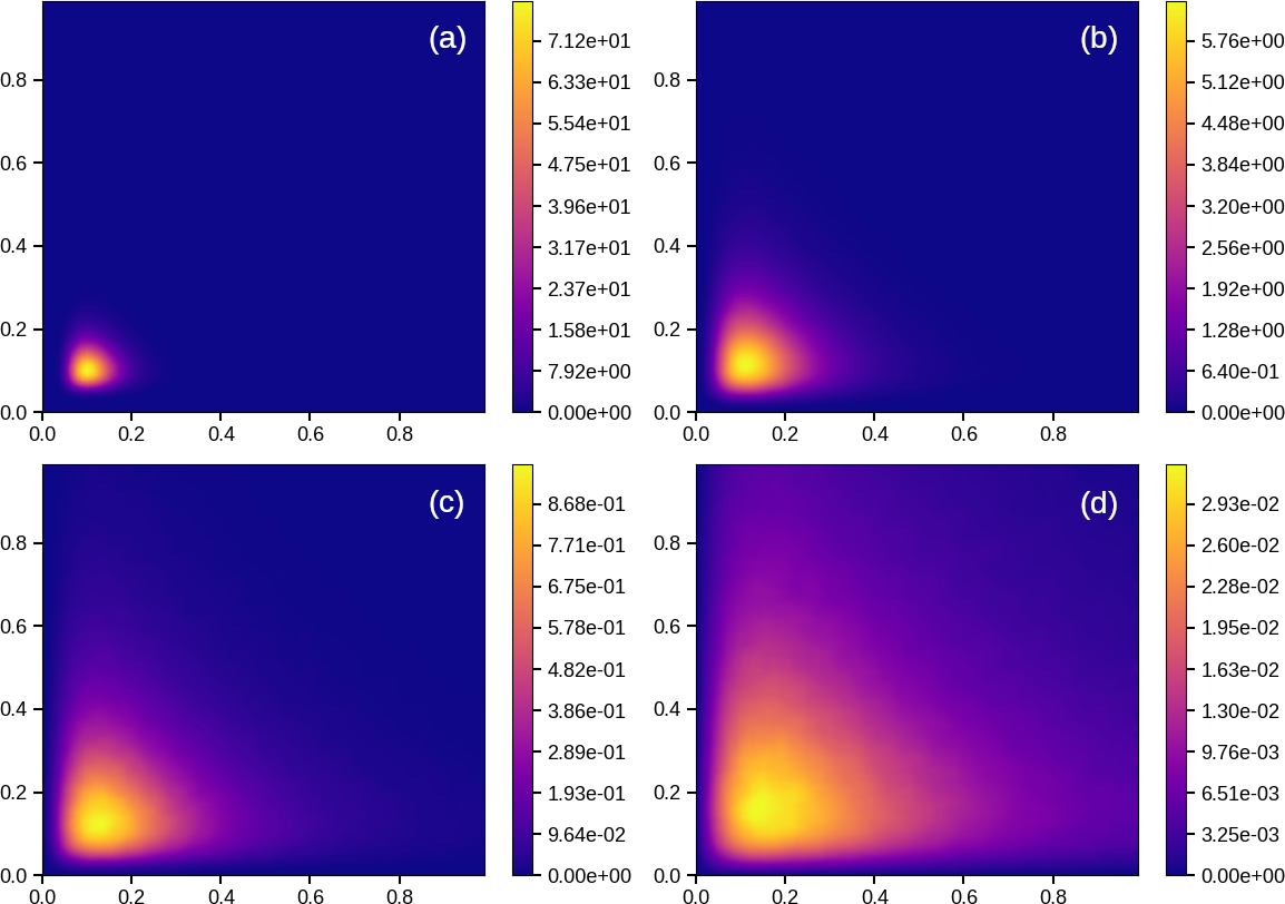
Stochastically estimated GF’s are plotted in Figure 8 at the four forward time instants: and For comparison, exact GF’s, determined from [20], are shown in Fig. 7. Again, quality Green’s function estimates are obtained at all four probed time instants, validating the use of forward time estimation. Again, under most circumstances, however, backward time estimation is recommended since one Green’s function estimate, obtained at a single response point, can be used in the magic rule to estimate the evolution of subject to any set of forcing conditions.
8 Discussion
When they can be found, Green’s functions provide a powerful tool for solving linear - and incrementally, nonlinear - evolution problems having the generic forms given by (1) and (2). Unfortunately, finding GF’s can be extremely difficult, particularly within geometrically complicated regions.
This paper proposes a numerical method for stochastically estimating GF’s, appropriate to diffusive and advective-dispersive/diffusive-reactive transport of scalar- and vector-valued quantities, e.g., convective heat and mass transfer problems involving passive, as well as chemically-reacting species. We validate the technique against three known GF’s, two that apply to simple diffusion in finite regions, and a third applicable to ground water transport in an infinite region. As formulated here, the stochastic Green’s function estimation technique can be applied to scalar transport in independently determined turbulent flows. More fundamentally, the technique might also be adapted to generate, in time-incremental fashion, GF’s for computing turbulent flows. In this case: i) the approach is limited to conditions where fluid particle momentum and vorticity dynamics are strongly Brownian, ii) the transported quantity corresponds to either local fluid momentum or vorticity [21], and iii) the turbulent flow problem is parabolic, evolving from a known initial condition.
We identify three principle challenges and propose straightforward solutions for each:
a) Since the probability of observing RW’s at Dirichlet boundaries is zero, RW’s that reach such boundaries must be removed. Random walker absorption, in turn, quickly compromises the quality of estimated GF’s. In order to address this problem, we introduce a random walker respawning technique which conserves the number of RW’s initially launched, as well as enforcing continuum mass conservation and diffusion at each respawning location.
b) Estimated Green’s functions exhibit spatial graininess, an artifact associated with use of discrete naive transition density estimators [38], Eq. (13). In order to solve this problem, as well as improve Green’s function estimation accuracy, we propose an area-averaging technique that bins neighboring Green’s function estimates, taken over small smoothing windows encompassing any given interrogation area, For most points, not near a boundary, the size of the smoothing window, is determined in iterative fashion by minimizing the point-wise deviation between numerical GF’s and averaged GF’s. In this first exploratory study, we use known rather than averaged GF’s in determining
c) To stochastically estimate Green’s functions, as given by Eq. (24) (no respawning, test 3) or (25) (with respawning, tests 1 and 2), three numerical parameters must be chosen: i) the number of RW’s, for forward time random walker integration), launched from the chosen solution/response point, [chosen impulse point, ii) the backward time-step size, [forward time-step size, and iii) the random walker interrogation area, Appendix A outlines approaches for determining these parameters; to the best of our knowledge, and beyond [44], the literature does not offer much guidance on this important practical question.
Although not treated in this paper, the proposed stochastic Green’s function construction technique provides a dual framework for tackling coupled particle and continuum transport problems, important, for example, in microscale bioheat and biomass transport problems [44], and a feature absent in BEM, GEM, and FEM formulations. The Green’s function estimation recipe shows that this particle-continuum duality arises from the connection between stochastic differential equations modeling particle-like transport and associated Fokker-Planck and backward Kolmogorov equations, probabilistically describing the same transport.
Acknowledgements
This work was supported by the Office of Naval Research, grant no. N00014-18-1-2754. Technical and coding support provided by Nikita Nikulsen is gratefully acknowledged.
References
- [1] K. Cole, J. Beck, A. Haji-Sheikh, B. Litkouhi, Heat Conduction Using Greens Functions, Series in Computational Methods and Physical Processes in Mechanics and Thermal Sciences, CRC Press, 2010.
- [2] G. Barton, Elements of Green’s functions and propagation: potentials, diffusion, and waves, Oxford University Press, 1989.
- [3] Y. Hon, M. Li, Y. Melnikov, Inverse source identification by green’s function, Engineering Analysis with Boundary Elements 34 (4) (2010) 352–358. doi:https://doi.org/10.1016/j.enganabound.2009.09.009.
- [4] J. Beck, B. Blackwell, A. Haji-Sheikh, Comparison of some inverse heat conduction methods using experimental data, International Journal of Heat and Mass Transfer 39 (17) (1996) 3649–3657. doi:https://doi.org/10.1016/0017-9310(96)00034-8.
- [5] A. P. Fernandes, M. B. dos Santos, G. Guimarães, An analytical transfer function method to solve inverse heat conduction problems, Applied Mathematical Modelling 39 (22) (2015) 6897–6914. doi:https://doi.org/10.1016/j.apm.2015.02.012.
- [6] D. Menemenlis, I. Fukumori, T. Lee, Using green’s functions to calibrate an ocean general circulation model, Monthly Weather Review 133 (2005) 1224–1240.
- [7] S. Boutami, S. Fan, Efficient pixel-by-pixel optimization of photonic devices utilizing the dyson’s equation in a green’s function formalism: Part i. implementation with the method of discrete dipole approximation, J. Opt. Soc. Am. B 36 (2019) 2378–2386.
- [8] S. Boutami, S. Fan, Efficient pixel-by-pixel optimization of photonic devices utilizing the dyson’s equation in a green’s function formalism: Part ii. implementation using standard electromagnetic solvers, J. Opt. Soc. Am. B 36 (2019) 2387–2394.
- [9] E. N. Economou, Green’s Functions in Quantum Physics, Springer Series in Solid-State Sciences, Springer, Berlin, 2006.
- [10] D. J. David Joseph Biagioni, Numerical construction of Green’s functions in high dimensional elliptic problems with variable coefficients and analysis of renewable energy data via sparse and separable approximations, Ph.D. Dissertation, Applied Mathemetics, University of Colorado, Boulder, 2012.
- [11] M. Costabel, Principles of boundary element methods, Computer Physics Reports 6 (1987) 243–274.
- [12] C. Brebbia, S. Walker, Boundary element techniques in engineering, Newnes-Butterworths, 1980.
- [13] A. E. Taigbenu, The green element method, International Journal for Numerical Methods in Engineering 38 (13) (1995) 2241–2263. doi:https://doi.org/10.1002/nme.1620381307.
- [14] Y. Wu, L. Cheng, S. Fang, S. Huang, P. Jia, A green element method-based discrete fracture model for simulation of the transient flow in heterogeneous fractured porous media, Advances in Water Resources 136 (2020) 103489. doi:https://doi.org/10.1016/j.advwatres.2019.103489.
- [15] P. Lorinczi, S. Harris, L. Elliott, Modelling of highly-heterogeneous media using a flux-vector-based green element method, Engineering Analysis with Boundary Elements 30 (2006) 818–833. doi:https://doi.org/10.1016/j.enganabound.2006.07.004.
- [16] O. C. Zienkiewicz, The finite element method in engineering science, McGraw-Hill, 1971.
- [17] K.-J. Bathe, Finite Element Method, John Wiley & Sons, Ltd, 2008. doi:https://doi.org/10.1002/9780470050118.ecse159.
- [18] D. J N Reddy, An Introduction to the Finite Element Method, McGraw-Hill Education, 2005.
- [19] T. Hughes, The Finite Element Method: Linear Static and Dynamic Finite Element Analysis, Dover Civil and Mechanical Engineering, Dover Publications, 2012.
- [20] A. Sanskrityayn, V. P. Singh, V. K. Bharati, N. Kumar, Analytical solution of two-dimensional advection–dispersion equation with spatio-temporal coefficients for point sources in an infinite medium using green’s function method, Environmental Fluid Mechanics 18 (3) (2018) 739–757.
- [21] R. G. Keanini, Green’s function-stochastic methods framework for probing nonlinear evolution problems: Burger’s equation, the nonlinear schrödinger’s equation, and hydrodynamic organization of near-molecular-scale vorticity, Annals of Physics 326 (4) (2011) 1002–1031.
- [22] M. Jovanovic, B. Bamieh, Modeling flow statistics using the linearized navier-stokes equations, in: Decision and Control, 2001. Proceedings of the 40th IEEE Conference on, Vol. 5, IEEE, 2001, pp. 4944–4949.
- [23] V. G. Levich, Physicochemical hydrodynamics, Prentice hall, 1962.
- [24] F. A. Williams, Combustion Theory: the fundamental theory of chemical reacting flow systems, Addison-Wesley, 1965.
- [25] P. Grindrod, The Theory and Applications of Reaction-diffusion Equations: Patterns and Waves, Oxford applied mathematics and computing science series, Clarendon Press, 1996.
- [26] A. Messiah, Quantum Mechanics, Dover Books on Physics, Dover Publications, 2014.
- [27] L. D. Landau, E. Lifshitz, L. Pitaevskij, Course of theoretical physics. vol. 10: Physical kinetics, Oxford, 1981.
-
[28]
G. Colonna, Boltzmann and
vlasov equations in plasma physics, in: Plasma Modeling, 2053-2563, IOP
Publishing, 2016, pp. 1–1 to 1–23.
doi:10.1088/978-0-7503-1200-4ch1.
URL http://dx.doi.org/10.1088/978-0-7503-1200-4ch1 - [29] G. B. Whitham, Linear and nonlinear waves, Vol. 42, John Wiley & Sons, 2011.
- [30] P. G. Drazin, R. S. Johnson, Solitons: an introduction, Vol. 2, Cambridge university press, 1989.
- [31] C. Gardiner, Handbook of Stochastic Methods for Physics, Chemistry, and the Natural Sciences, Springer complexity, Springer, 2004.
- [32] M. E. Muller, Some continuous monte carlo methods for the dirichlet problem, The Annals of Mathematical Statistics 27 569–589.
- [33] K. K. Sabelfeld, Monte Carlo methods in boundary value problems, Springer series in computational physics, Springer, Berlin, 1991.
- [34] T. E. Booth, Exact monte carlo solution of elliptic partial differential equations, Journal of Computational Physics 39 (1981) 396–404. doi:10.1016/0021-9991(81)90159-5.
- [35] K. K. Sabelfeld, N. A. Simonov, Random walks on boundary for solving PDEs, De Gruyter, 2013.
- [36] A. Haji-Sheikh, E. M. Sparrow, The floating random walk and its application to monte carlo solutions of heat equations, SIAM Journal on Applied Mathematics 14 (2) (1966) 370–389.
- [37] M. Mascagni, N. A. Simonov, Monte carlo methods for calculating some physical properties of large molecules, SIAM journal on scientific computing 26 (1) (2004) 339–357.
- [38] B. W. Silverman, Density Estimation for Statistics and Data Analysis, Chapman & Hall, 1986.
- [39] G. N. Milstein, J. G. M. Schoenmakers, V. Spokoiny, Transition density estimation for stochastic differential equations via forward-reverse representations, Bernoulli 10 (2004) 281–312.
- [40] L. Devroye, L. Gyorfi, Nonparametric Density Estimation: The L1 View, Wiley Interscience Series in Discrete Mathematics, Wiley, 1985.
- [41] E. Olariu, K. K. Cadwell, E. Hancock, D. Trueman, H. Chevrou-Severac, Current recommendations on the estimation of transition probabilities in markov cohort models for use in health care decision-making: a targeted literature review, Clinicoecon Outcomes Res. 9 (2017) 537–546.
- [42] M. Rudemo, Empirical choice of histograms and kernel density estimators, Scandinavian Journal of Statistics 9 (1982) 65–78.
- [43] Z. Schuss, Theory and Applications of Stochastic Processes: An Analytical Approach, Applied Mathematical Sciences, Springer New York, 2009.
-
[44]
Z. Schuss, Brownian
Dynamics at Boundaries and Interfaces: In Physics, Chemistry, and Biology,
Applied Mathematical Sciences, Springer New York, 2013.
URL https://books.google.com/books?id=eOi3BAAAQBAJ - [45] G. N. Milstein, Approximate integration of stochastic differential equations, Theory of Probability & Its Applications 19 (1975) 557–562.
- [46] G. Milstein, Numerical Integration of Stochastic Differential Equations, Mathematics and Its Applications, Springer Netherlands, 1994.
- [47] P. E. Kloeden, E. Platen, Numerical Solution of Stochastic Differential Equations, Stochastic Modelling and Applied Probability, Springer Berlin Heidelberg, 2011.
- [48] J. A. Hansen, C. Penland, Efficient approximate techniques for integrating stochastic differential equations, Monthly Weather Review 134 (2006) 3006 – 3014. doi:10.1175/MWR3192.1.
- [49] T. Sauer, Numerical solution of stochastic differential equations in finance (2012) 529–550.
- [50] S. Ulam, R. Richtmyer, J. von Neumann, Statistical methods in neutron diffusion, Los Alamos Scientific Laboratory report LAMS–551 (1947).
- [51] N. Metropolis, S. Ulam, The monte carlo method, J. Amer. Stat. Assn. 44 (1949) 335–341.
- [52] J. Todd, Experiments in the solution of differential equations by monte carlo methods, J. Washington Acad. Sci. 12 (1954) 377–381.
- [53] I. Dimnov, D. McKee, Monte Carlo Methods for Applied Scientists, World Scientific, 1998.
- [54] R. Feynman, Principles of Least Action in Quantum Mechanics, Ph.D. Dissertation, Physics, Princeton University, 1942.
- [55] M. Kac, On distributions of certain wiener functionals, Trans. Amer. Math. Soc. 65 (1949) 1–13.
- [56] M. Kac, On some connections between probability theory and differential and integral equations (1951) 189–215.
- [57] A. Friedman, Stochastic differential equations and applications, Vol. 1, Academic Press, 1975.
- [58] R. Bass, Stochastic Processes, Cambridge Univ. Press, 2011.
- [59] D. Forster, Hydrodynamic Fluctuations, Broken Symmetry, And Correlation Functions, CRC Press, 2018.
- [60] J. Boon, S. Yip, Molecular Hydrodynamics, McGraw-Hill, 1980.
- [61] M. Toda, R. Kubo, N. Saito, N. Hashitsume, Statistical Physics II: Nonequilibrium Statistical Mechanics, Springer Series in Solid-State Sciences, Springer Berlin Heidelberg, 2012.
- [62] I. Lux, L. Koblinger, Monte Carlo Particle Transport Methods: Neutron and Photon Calculations (1st ed.), CRC Press, 1991.
- [63] J. Bear, A. Cheng, Modeling Groundwater Flow and Contaminant Transport, Springer, 2010.
Supporting information
S1
Appendices to ’Stochastic estimation of Green’s functions with application to advection-diffusion-reaction problems’
S1 Appendix A
Choosing the number of RW’s launched, interrogation area, and the time step, The stochastic estimation technique requires specification of three numerical parameters: i) the backward (forward) time-step size, ii) the interrogation area, and iii) the number of RW’s, launched from the chosen GF solution point, Since the literature appears to offer little guidance on choosing these parameters, and since the choices require some experimentation, we propose two straightforward approaches for identifying appropriate values. Here, we outline the technique used in this study. We focus on the simplest case in which the diffusion tensor is uniform and isotropic, It is important to recognize that in both approaches, some numerical experimentation is required.
In order to address these important questions, we focus on forward-time integration of RW trajectories:
| (40) |
and highlight two features: a) the connection between and and b) minimization of early-time variance in the number of RW’s captured on
For simplicity, limit attention to two-dimensional diffusive transport of Spatially resolved random walker displacements, over require Thus, we choose
| (41) |
where this choice represents the smallest area allowing statistically acceptable sampling of If is chosen smaller than then for any given number of RW’s launched from a number of RW’s located near at forward instant will (numerically) jump over/around at The result is an underestimated Likewise, if is chosen larger than the number captured on is too large, overestimating
In order to determine acceptable consider the time-dependent standard deviation, in in the number of RW’s captured by the set of interrogation areas, lying on the circle, centered on the launch location,
| (42) |
where is the mean penetration radius of the RW’s launched from at time and
The number of interrogation areas lying on is given approximately by:
| (43) |
where, in the case that the the spatial domain is discretized into uniform interrogation areas, with Since then
| (44) |
From Eq. (42), and for small interrogation areas, being the area of the solution domain,
| (45) |
From this expression, it becomes apparent that the maximum spatial variation, in random walker capture numbers, occurs at where
In order determine an acceptable we calculate the ratio of the mean number of RW’s captured at to
| (46) | ||||
or
| (47) |
where represents, e.g., the centroid of the interrogation area, lying on and where
Finally, solving for we obtain the maximum relative spatial variation in captured RW’s, expressed as a function of and
| (48) |
Thus, the following procedure can be used to determine and
a) Based on the nature of the transport problem under study, identify the spatial resolution required; this choice determines and
b) Use Eq. (41) to determine for problems where
c) Choose a desired maximum relative (spatial, early-time) variation in RW’s captured on and solve Eq. (48) for
Note 1: Since all RW’s are independent, one can effectively increase the number of RW’s launched from a given solution point, - which, for single-swarm simulations, we denote as - by relaunching another swarm of RW’s from the same point. The number used in the relaunch, can be larger or smaller than the corresponding numbers of RW’s captured in each interrogation area, and respectively, can then be pooled to improve GF estimation accuracy.
Note 2: As long as dimensional lengths are scaled by the either the short-time or long-time diffusion length scales, or where is the chosen solution time interval, this procedure applies for GF estimation procedures cast in either dimensional or nondimensional form.
S1 Appendix B
Properties of the respawning algorithm. In order to focus on the computational challenges associated with absorbing boundaries, in this subsection we limit attention to pure diffusion problems in which no advection takes place. Thus, the backward-time velocity field, is set to zero. The proposed respawning algorithm has three properties that appear to be essential to estimating low-error GF’s within bounded domains:
a) At all times and all locations in the solution domain, and with an error on the order of the algorithm conserves random walker mass, which, in turn, enforces the adjoint equation, (26).
In order to show that the respawning algorithm enforces the adjoint equation, label the location where the random walker having maximum weight at any instant as Define a local system, having origin at such that the is aligned with the local gradient vector, in the random walker mass density field, The continuous field, can be constructed, for example, by interpolation on the discrete instantaneous distribution of weighted RW’s.
The process of removing a maximum-weight random walker, having weight located at and replacing it with two RW’s, each of weight and both placed at can be represented by the following expression:
| (49) |
random walker mass is clearly conserved since the left hand side of (49) is identically zero. Taylor expanding the first term in the positive direction, the second term in the negative direction, and rearranging, we obtain:
| (50) |
where, in the limit with and where the order of discretization error is as shown.
Finally, expressing the left hand side of (50) as a temporal Taylor expansion about and the two terms on the right as spatial expansions about we obtain the local mass diffusion equation, evaluated at and expressed in the backward time direction
| (51) |
Note, that replacing the time index with shifts evaluation of (51) to
b) If we use the RW’s to model physical Brownian particles, and the respawning algorithm to model some process by which the particles can undergo binary fission, we see that it enforces the diffusion equation (51) in the direction of the local random walker mass flux, Since physical particles, unlike numerical RW’s, cannot both occupy the same point that their parent occupied, we would introduce a spatial offset for the respawned RW’s. Thus, the fission of any given set of maximum-weight RW’s, produces a mass gradient at each of the respawning locations, and the algorithm, in effect, smooths - on short (single-time-step) time-scales, - localized, and randomly-distributed (in space) removal of random walker mass. Hence, the algorithm appears to be insensitive to the method used to reorder, at the end of every time-steps, the weight array, Although this remains an open question, our results strongly support this view.
c) As noted in the article, the third property associated with the respawning algorithm centers on the fact that it conserves the number of RW’s launched from the solution point, As shown in the article, this property ensures that accurate GF estimates can be obtained throughout any given time interval,
S1 Appendix C
Illustration of trial and error derivation of the adjoint equation and magic rule. A technical hurdle that likely limits widespread use of GF’s, particularly among non-specialists, revolves around the origins of the adjoint equation governing the Green’s function, and the so-called ’magic rule’ [barton], the integral solution for the transport variable, Since textbooks and research articles appear to be universally mute on how these essential building blocks are obtained - specifically, not showing how they can be simultaneously derived via straightforward trial and error - we illustrate trial and error determination of these the adjoint equation and magic rule, focusing for simplicity on fixed diffusivity advection-diffusion problems, evolving in incompressible flow fields:
| (52) |
The procedure incorporates four steps, the first of which is generally not highlighted: a) guess the form of the adjoint equation, b) multiply the candidate adjoint equation by and the transport equation, Eq. (52) by the Green’s function, c) integrate both equations in b) over the space-time hypersurface, formed by the product of the problem’s spatial boundary, and the time axis, and d) taking the difference of the integral equations in c), use Green’s theorems and trial and error alteration of the guessed adjoint equation to arrive at an integral solution for stated strictly in terms of space-time surface integrals over the former involving derivatives of and known boundary and initial conditions.
In step a), it’s generally good strategy to guess that the adjoint equation has the same generic form as the transport equation, Eq. (52), but with one or more signs reversed, and with the source term, replaced by
| (53) |
where: i) we have arbitrarily guessed that all signs on the left of the adjoint equation are positive, and ii) have fixed the solution point, Choice ii): a) leads, in straightforward fashion, to an isolated term, at the end of the procedure, and b) means that the space-time integrals formed in step c) are taken over and
Carrying out steps b) and c), we obtain:
| (54) |
where and where the upper limit on the time integrals, is set just beyond as shown in Eq. (55) below, following time integration, this trick suppresses the a priori unknown integral at In addition, it allows exposure of from the first right-hand term in Eq. (S1 Appendix C).
Moving to step d) and focusing on Eq. (S1 Appendix C), use Liebniz rule on the fourth term on the left and combine with the first:
| (55) |
Using the property that is undefined at for the first term simplifies to where is the specified initial condition. Since the line (d=2) or area (d=3) integral in the second term of Eq. (55) must be suppressed, we see that the guessed plus sign on the first term in Eq. (53) must be changed to a minus.
Using similar steps on the two advective terms on the left side of Eq. (S1 Appendix C (terms 2 and 5) yields:
| (56) |
where, for incompressible flow, allowing the in term 5, Eq. (S1 Appendix C) to be brought in front of the divergence operator: Both area (d=2) or volume (d=3) integrals in Eq. (56) are a priori unknown. The first can be restated as a known/calculable line (d=2) or area (d=3) integral via the divergence theorem. The second, however, must again be suppressed by changing the guessed plus sign on term 2, Eq. (53), to a minus. Thus, the two terms in Eq. (56) simplify to:
| (57) |
where denotes the advective (inflow plus outflow) boundaries of and where and are assumed known, at all times and locations on In addition, is the outward unit normal to Finally, focusing on terms 3 and 6 in Eq. (S1 Appendix C), we are again lead to an a priori unknown surface/volume (d=2/3) integral:
| (58) |
In order to suppress this term, we change the plus sign on the third term in Eq. (53) to a negative. Using the divergence theorem and integration by parts, introducing the three sign changes above into the guessed adjoint equation, Eq. (53), labeling the functions associated with specified Dirichlet, Neumann, and initial conditions on respectively, as and and choosing the plus sign on the first term of the right side of Eq. (S1 Appendix C), we finally obtain the magic rule:
| (59) |
where and correspond, respectively, to the portions of the domain boundary, on which Dirichlet, Neumann, and inflow/outflow boundary conditions are imposed, and where is the spatially and temporally specified value of on the Dirichlet boundary.
S1 Appendix D
Extraction of the transport equation, Eq. (37), associated with the Green’s function in test 3. The transition density estimated in test 3, governed by the Fokker-Planck equation, Eq. (34), also satisfies the backward Kolmogorov equation:
| (60) |
where and are expressed in terms of variable ’backward’ variables, and