Stochastic Galerkin methods for linear stability analysis of systems with parametric uncertainty††thanks: This work was supported by the U. S. National Science Foundation under grant DMS1913201.
Abstract
We present a method for linear stability analysis of systems with parametric uncertainty formulated in the stochastic Galerkin framework. Specifically, we assume that for a model partial differential equation, the parameter is given in the form of generalized polynomial chaos expansion. The stability analysis leads to the solution of a stochastic eigenvalue problem, and we wish to characterize the rightmost eigenvalue. We focus, in particular, on problems with nonsymmetric matrix operators, for which the eigenvalue of interest may be a complex conjugate pair, and we develop methods for their efficient solution. These methods are based on inexact, line-search Newton iteration, which entails use of preconditioned GMRES. The method is applied to linear stability analysis of Navier–Stokes equation with stochastic viscosity, its accuracy is compared to that of Monte Carlo and stochastic collocation, and the efficiency is illustrated by numerical experiments.
keywords:
linear stability, eigenvalue analysis, uncertainty quantification, spectral stochastic finite element method, Navier–Stokes equation, preconditioning, stochastic Galerkin methodAMS:
35R60, 60H15, 65F15, 65L07, 65N22, 65N251 Introduction
The identification of instability in large-scale dynamical system is important in a number of applications such as fluid dynamics, epidemic models, pharmacokinetics, analysis of power systems and power grid, or quantum mechanics and plasma physics. A steady solution is stable, if when in a transient simulation it is introduced with a small perturbation as initial data and the simulation reverts to , and it is unstable otherwise. This is of fundamental importance since unstable solutions may lead to inexplicable dynamic behavior. Linear stability analysis entails computing the rightmost eigenvalue of the Jacobian evaluated at , and thus it leads to solution of, in general, large sparse generalized eigenvalues problems see, e.g. [4, 6, 8, 13, 16, 27] and the references therein. Typically, a complex pair of rightmost eigenvalues leads to a Hopf bifurcation, and a real rightmost eigenvalue may lead to a pitchfork bifurcation. The analysis is further complicated if the parameters in the systems are functions of one or more random variables. This is quite common in many real-world applications, since the precise values of model coefficients or boundary conditions are often not known. A popular method for this type of problems is Monte Carlo, which is known for its robustness but also slow convergence. In this study, we use spectral stochastic finite element methods [12, 17, 33, 34] with the main focus on the so-called stochastic Galerkin method, for the linear stability analysis of Navier–Stokes equation with stochastic viscosity. Specifically, we consider the parameterized viscosity given in the form of generalized polynomial chaos (gPC) expansion. In the first step, we apply the algorithms developed in [18, 30], see also [24], to find a gPC expansion of the solution of the Navier–Stokes equation. In the second step, we use the expansions of the solution and viscosity to set up a generalized eigenvalue problem with a nonsymmetric matrix operator, and in the assessment of linear stability of this problem we identify the gPC expansions of the rightmost eigenvalue. The main contribution in this study is development of stochastic Galerkin method for nonsymmetric eigenvalue problems. Our approach is based on inexact Newton iteration: the linear systems with Jacobian matrices are solved using GMRES, for which we also develop several preconditioners. The preconditioners are motivated by our prior work on (truncated) hierarchical preconditioning [32, 19], see also [2]. For an overview of literature on solving eigenvalue problems in the context of spectral stochastic finite element methods we refer to [1, 19, 29] and the references therein. Recently, Hakula and Laaksonen [15] studied crossing of eigenmodes in the stochastic parameter space, and Elman and Su [9] developed a low-rank inverse subspace iteration. However, to the best of our knowledge, there are only a few references addressing nonsymmetric stochastic eigenvalue problems: by Sarrouy et al. [25, 26], but there is no discussion of efficient solution strategies, and also by Sonday et al. [28], who studied distribution of eigenvalues for the Jacobian in the context of stochastic Galerkin method. Most recently, the authors with collaborators also compared surrogate learning strategies based on a sampling method, Gaussian process regression and a neural network in [31].
A study of linear stability of Navier–Stokes equation under uncertainty was conducted by Elman and Silvester [5]. The study was based on a judiciously chosen perturbation of the state variable and a stochastic collocation method was used to characterize the rightmost eigenvalue. Our approach here is different. We consider parametric uncertainty (of the viscosity), and the solution strategy is based on the stochastic Galerkin method. In fact, also the variant of the collocation method used here is based on the stochastic Galerkin projection (sometimes called a nonintrusive stochastic Galerkin method in the literature, see [33, Chapter 7] for a discussion). From this perspective, our study can be viewed as an extension of the setup from [6] to problems with viscosity given in the form of stochastic expansion and their efficient solution using stochastic Galerkin method. However, more importantly, we illustrate that the inexact methods for stochastic eigenvalue problems proposed recently by Lee and Sousedík [19] can be also applied to problems with nonsymmetric matrix operator111Specifically, the methods based on inexact Newton iteration, since in our experience the stochastic Rayleigh quotient and inverse iteration methods are less effective for nonsymmetric problems.. This in general allows to perform a linear stability analysis for other types of problems as well. We do not address eigenvalue crossing here, which is a somewhat delicate task for gPC-based techniques. We assume that the eigenvalue of interest is sufficiently separated from the rest of the spectrum and no crossing occurs. This is often the case for outliers and other eigenvalues that may be of interest in applications. A suitability of the algorithm we propose in this study can be assessed, e.g., by running first a low-fidelity (quasi-)Monte Carlo simulation. We also note that from our experience with the problem at hand indicates that the rightmost eigenvalue remains relatively well separated from the rest of the spectrum, and it is less prone to switching unlike the other eigenvalues, even with moderate values of coefficient of variation, which in turn allows its efficient characterization by a gPC expansion.
The rest of the paper is organized as follows. In Section 2 we recall the basic elements of linear stability analysis and link it to an eigenvalue problem for a specific model given by Navier–Stokes equation, in Section 3 we introduce the stochastic eigenvalue problem, in Section 4 we formulate the sampling methods and in Section 5 the stochastic Galerkin method and inexact Newton iteration for its solution, in Section 6 we apply the algorithms to linear stability analysis of Navier–Stokes equation with stochastic viscosity, in Section 7 we report the results of numerical experiments, and finally in Section 8 we summarize and conclude our work.
2 Linear stability and deterministic model problem
Following [6], let us consider the dynamical system
| (1) |
where is a nonlinear mapping, is the state variable (velocity, pressure, temperature, deformation, etc.), in the finite element setting is the mass matrix, and is a parameter. Let denote the steady-state solution to (1), i.e., . We are interested in the stability of: if a small perturbation is introduced to at time , does grow with time, or does it decay? For a fixed value of , linear stability of the steady-state solution is determined by the spectrum of the eigenvalue problem
| (2) |
where is the Jacobian matrix of evaluated at . The eigenvalues have a general form , where and . Then , and since , there are in general two cases: if the perturbation decays with time, and if the perturbation grows. We refer, e.g., to [4, 13] and the references therein for a detailed discussion. That is, if all the eigenvalues have strictly negative real part, then is a stable steady solution, and if some eigenvalues have nonnegative real part, then is unstable. Therefore, a change of stability can be detected by monitoring the rightmost eigenvalues of (2). A steady-state solution may lose its stability in one of two ways: either the rightmost eigenvalue of (2) is real and passes through zero from negative to positive as varies, or (2) has a complex pair of rightmost eigenvalues and they cross the imaginary axis as varies, which leads to a Hopf bifurcation with the consequent birth of periodic solutions of (1).
Consider a special case of (1), the time-dependent Navier–Stokes equations governing viscous incompressible flow,
| (3) | ||||
subject to appropriate boundary and initial conditions in a bounded physical domain, where is the kinematic viscosity, is the velocity and is the pressure. Properties of the flow are usually characterized by the Reynolds number
where is the characteristic velocity and is the characteristic length. For convenience, we will also sometimes refer to the Reynolds number instead of the viscosity. Mixed finite element discretization of (3) gives the following Jacobian and the mass matrix, see [6] and [8, Chapter ] for more details,
| (4) |
where is the number of velocity and pressure degrees of freedom, respectively, , is nonsymmetric, is the divergence matrix, and the velocity mass matrix is symmetric positive definite. The matrices are sparse and is typically large. We note that the mass matrix is singular, and (2) has an infinite eigenvalue. As suggested in [3], we replace the singular mass matrix with the nonsingular, shifted mass matrix
| (5) |
which is symmetric but in general indefinite, and it maps the infinite eigenvalues of (2) to and leaves the finite ones unchanged. Then, the generalized eigenvalue problem (2) can be transformed into an eigenvalue problem
| (6) |
The flow is considered stable if , and we wish to detect the onset of instability, that is to find when the rightmost eigenvalue crosses the imaginary axis. Efficient methods for finding the rightmost pair of complex eigenvalues of (2) (or (6)) were studied in [6]. Here, our goal is different. We consider parametric uncertainty in the sense that the parameter , where is a set of random variables and which is given by the so-called generalized polynomial chaos expansion. To this end, we first recast the eigenvalue problem (6) in the spectral stochastic finite element framework, then we show how to efficiently solve it, and finally we apply the stability analysis to Navier–Stokes equation with stochastic viscosity.
3 Stochastic eigenvalue problem
Let be a complete probability space, that is is the sample space with -algebra and probability measure. We assume that the randomness in the mathematical model is induced by a vector of independent random variables , where . Let denote the Borel -algebra on induced by and the induced measure. The expected value of the product of measurable functions on determines a Hilbert space with inner product
| (7) |
where the symbol denotes the mathematical expectation.
In computations we will use a finite-dimensional subspace spanned by a set of multivariate polynomials that are orthonormal with respect to the density function , that is , and is constant. This will be referred to as the gPC basis [34]. The dimension of the space, depends on the polynomial degree. For polynomials of total degree, the dimension is .
Suppose that we are given an affine expansion of a matrix operator, which may correspond to the Jacobian matrix in (2), as
| (8) |
where each is a deterministic matrix, and is the mean-value matrix . The representation (8) is obtained from either Karhunen-Loève or, more generally, a stochastic expansion of an underlying random process; a specific example is provided in Section 7.
We are interested in a solution of the following stochastic eigenvalue problem: find a specific eigenvalue and possibly also the corresponding eigenvector, which satisfy in almost surely (a.s.) the equation
| (9) |
where is a nonsymmetric matrix operator, is a deterministic mass matrix, and along with a normalization condition
| (10) |
which is further specified in Section 5.
We will search for expansions of the eigenpair in the form
| (11) |
where and are coefficients corresponding to the basis. We note that the series for in (11) converges for in the space under the assumption that the gPC polynomials provide its orthonormal basis and provided that has finite second moments see, e.g., [10] or [33, Chapter 5]. Convergence analysis of this approximation for self-adjoint problems can be found in [1].
4 Monte Carlo and stochastic collocation
Both Monte Carlo and stochastic collocation are based on sampling. The coefficients are defined by a discrete projection
| (12) |
The evaluations of coefficients in (12) entail solving a set of independent deterministic eigenvalue problems at a set of sample points, or ,
| (13) |
In the Monte Carlo method, the sample points, are generated randomly following the distribution of the random variables, , and moments of solution are computed by ensemble averaging. In addition, the coefficients in (11) could be computed using Monte Carlo integration as222In numerical experiments, we avoid this approximation of the gPC coefficients and directly work with the sampled quantities.
For stochastic collocation, which is used here as the so-called nonintrusive stochastic Galerkin method, the sample points, consist of a predetermined set of collocation points, and the coefficients and in the expansions (11) are determined by evaluating (12) in the sense of (7) using numerical quadrature as
where are the quadrature (collocation) points and are quadrature weights. Details of the rule we use in our numerical experiments are discussed in Section 7, and we refer to monograph [17] for a detailed discussion of quadrature rules.
5 Stochastic Galerkin method and Newton iteration
The stochastic Galerkin method is based on the projection
| (14) | ||||||
| (15) |
Let us introduce the notation
| (16) |
In order to formulate an efficient algorithm for eigenvalue problem (9) with nonsymmetric matrix operator using the stochastic Galerkin formulation, we introduce a separated representation of the eigenpair using real and imaginary parts,
where and . Then, replacing and in eigenvalue problem (9) results in
| (17) |
Expanding the terms in (17) and collecting the real and imaginary parts yields a system of equations that can be written in a separated representation as
| (18) |
and the normalization condition corresponding to the separated representation in (18) is taken as
| (19) |
Now, we seek expansions of type (11) for , , , and , that is
| (20) |
where the symbol denotes the Kronecker product, , , and for .
Let us consider expansions (20) as approximations to the solution of (18)–(19). Then, we can write the residual of (18) as
and the residual of (19) as
Imposing the stochastic Galerkin orthogonality conditions (14) and (15) to and, respectively, we get a system of nonlinear equations
| (21) |
where
and
We will use Newton iteration to solve system of nonlinear equations (21). The Jacobian matrix of (21) can be written as
where
| (22) | ||||
| (23) |
and
| (24) | ||||
| (25) |
However, for convenience in the formulation of the preconditioners presented later, we formulate Newton iteration with rescaled Jacobian matrix, which at step entails solving a linear system
| (26) |
followed by an update
| (27) |
Remark 1.
Linear systems (26) are solved inexactly using a preconditioned GMRES method. We refer to Appendix A for the details of evaluation of the right-hand side and of the matrix-vector product, and to [18] for a discussion of GMRES in a related context.
5.1 Inexact Newton iteration
As in [19], we consider a line-search modification of this method following [23, Algorithm 11.4] in order to improve global convergence behavior of Newton iteration. Denoting
we define the merit function as the sum of squares,
that is is the negative right-hand side of (26), i.e., it is a rescaled residual of (21), and we also denote
As the initial approximation of the solution, we use the eigenvectors and eigenvalues of the associated mean problem
| (28) |
concatenated by zeros, that is
and the initial residual is
The line-search Newton method is summarized in our setting as Algorithm 1, and the choice of parameters and in the numerical experiments is discussed in Section 7.
The inexact iteration entails in each step a solution of the stochastic Galerkin linear system in Line 4 of Algorithm 1 given by (26) using a Krylov subspace method. We use preconditioned GMRES with the adaptive stopping criteria,
| (29) |
where . The for-loop is terminated when the convergence check in Line 12 is satisfied; in our numerical experiments we check if .
Our implementation of the solvers is based on the so-called matricized formulation, in which we make use of isomorphism between and determined by the operators and : , (, where , . The upper/lower case notation is assumed throughout the paper, so (, etc. Specifically, we define the matricized coefficients of the eigenvector expansion
| (30) |
where the column contains the coefficients associated with the basis function. A detailed formulation of the GMRES in the matricized format can be found, e.g., in [18]. We only describe computation of the matrix-vector product (Appendix A), and in the next section we formulate several preconditioners.
5.2 Preconditioners for the Newton iteration
In order to allow for an efficient iterative solution of linear systems in Line 4 of Algorithm 1 given by (26) using a Krylov subspace method, it is necessary to provide a preconditioner. In this section, we adapt the mean-based preconditioner and two of the constraint preconditioners from [19] to the formulation with separated real and complex parts, and we write them in the matricized format. The idea can be motivated as follows. The preconditioners are based on approximations of the blocks in (45). The mean-based preconditioner is inspired by the approximation
where and the Schur complement . The constraint preconditioners are based on the approximation
where and . Next, considering the truncation of the series in (46)–(51) to the very first term, we get
The precise formulations are listed for the mean-based preconditioner as Algorithm 2 and for the constraint mean-based preconditioner as Algorithm 3. Finally, the constraint hierarchical Gauss-Seidel preconditioner is listed as Algorithm 4. It can be viewed as an extension of Algorithm 3, because the solves with stochastic Galerkin matrices (35) are used also in this preconditioner, but in addition the right-hand sides are updated using an idea inspired by Gauss-Seidel method in a for-loop over the degree of the gPC basis. Moreover, as proposed in [32], the matrix-vector multiplications, used in the setup of the right-hand sides can be truncated in the sense that in the summations, is replaced by , where with for some , and in particular with the chGS preconditioner (Algorithm 4) reduces to the cMB preconditioner (Algorithm 3). We also note that, since the initial guess is zero in Algorithm 4, the multiplications by and vanish from (36)–(37).
The preconditioner is defined as
| (31) |
Above
| (32) |
where and are the real and imaginary components of eigenvector of the stencil with corresponding eigenvalue +i, cf. (28), and
| (33) |
with constants , further specified in the numerical experiments section.
5.2.1 Updating the constraint preconditioner
It is also possible to update the application of the constraint mean-based preconditioner in order to incorporate the latest approximations of the eigenvector mean coefficients represented by the vectors in (35). Suppose the inverse of the matrix from (35) for is available, e.g., as the LU decomposition. That is, we have the preconditioner for the initial step of the Newton iteration, and let us denote its application by . Specifically, , where and are the factors of. Next, let us consider two matrices and such that
| (38) |
where
Specifically, is the rank update of the preconditioner at step of Newton iteration, and the matrices and can be computed using a sparse SVD, which is available, e.g., in [20]. In implementation, using Matlab notation with , we compute and set , . Finally, a solve at step of Newton iteration may be facilitated using the Sherman-Morrison-Woodbury formula see, e.g. [14], or [22, Section 3.8], as
6 Bifurcation analysis of Navier–Stokes equations with stochastic viscosity
Here, we follow the setup from [30] and assume that the viscosity is given by a stochastic expansion
| (39) |
where is a set of given deterministic spatial functions. We note that there are several possible interpretations of such setup [24, 30]. Assuming fixed geometry, the stochastic viscosity is equivalent to Reynolds number being stochastic and, for example, to a scenario when the volume of fluid moving into a channel is uncertain. Consider the discretization of (3) by a div-stable mixed finite element method, and let the bases for the velocity and pressure spaces be denoted and , respectively. We further assume that we have a discrete approximation of the steady-state solution of the stochastic counterpart of (3), given as333Techniques for computing these approximations were studied in [18, 30].
We are interested in a stochastic counterpart of the generalized eigenvalue problem (2), which we write as
| (40) |
where is the deterministic (shifted) mass matrix from (5), and is the stochastic Jacobian matrix operator given by the stochastic expansion
| (41) |
The expansion is built from matrices , , such that
where , and is a sum of the vector-Laplacian matrix, the vector-convection matrix, and the Newton derivative matrix ,
where
and if , we set for , and if , we set for . In the numerical experiments, we use the stochastic Galerkin method from [30] to calculate the terms for the construction of the matrices . The divergence matrix is defined as
and the velocity mass matrix is defined as
7 Numerical experiments
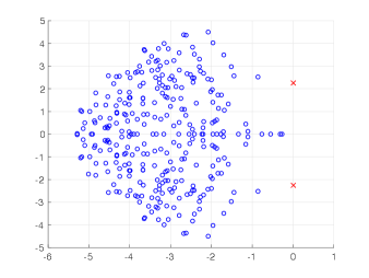
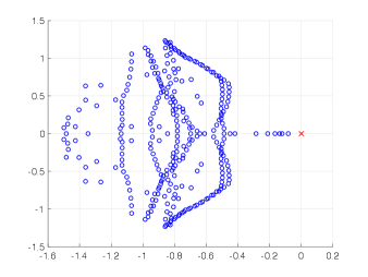
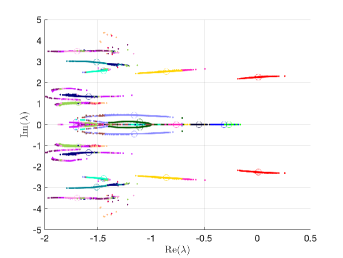
We implemented the method in Matlab using IFISS 3.5 package [7], and we tested the algorithms using two benchmark problems: flow around an obstacle and an expansion flow around a symmetric step. The stochastic Galerkin methods were used to solve both the Navier–Stokes problem (see [18, 30] for full description) and the eigenvalue problem (9), which was solved using the inexact Newton iteration from Section 5. The sampling methods (Monte Carlo and stochastic collocation) entail generating a set of sample viscosities from (39), and for each sample solving a deterministic steady-state Navier–Stokes equation followed by a solution of a deterministic eigenvalue problem (13) with a matrix operator corresponding to sampled Jacobian matrix operator (41), where the deterministic eigenvalue problems at sample points were solved using function eigs in Matlab. For the solution of the Navier–Stokes equation, in both sampling and stochastic Galerkin methods, we used a hybrid strategy in which an initial approximation was obtained from solution of the stochastic Stokes problem, after which several steps of Picard iteration were used to improve the solution, followed by Newton iteration. A convergent iteration stopped when the Euclidean norm of the algebraic residual was smaller than , see [30] for more details. Also, when replacing the mass matrix by the shifted mass matrix, see (4) and (5), we set as in [6]. The eigenvalues with the largest real part of the deterministic eigenvalue problem with mean viscosity for each of the two examples are displayed in Figure 1.
 |
 |
7.1 Flow around an obstacle
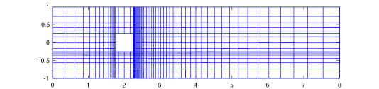
For the first example, we considered flow around an obstacle in a similar setup as studied in [30]. The domain of the channel and the discretization are shown in Figure 2. The spatial discretization used a stretched grid with QQ1 finite elements. We note that these elements are referred to as Taylor-Hood in the literature. There were velocity and pressure degrees of freedom. The viscosity was taken to be a truncated lognormal process transformed from the underlying Gaussian process [11]. That is, , , is a set of Hermite polynomials and, denoting the coefficients of the Karhunen-Loève expansion of the Gaussian process by and , the coefficients in expansion (39) were computed as
The covariance function of the Gaussian field, for points and in, was chosen to be
| (42) |
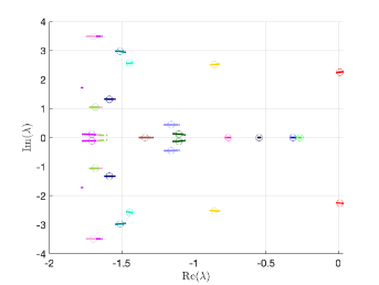
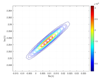
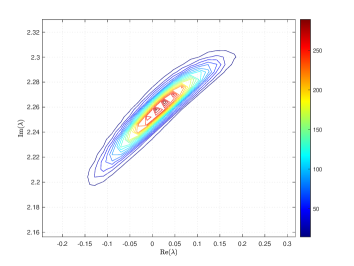
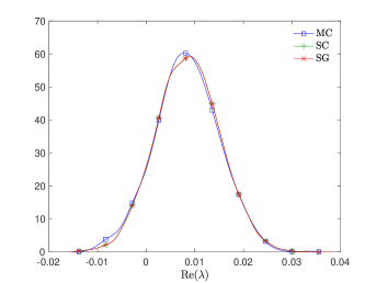
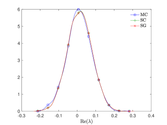
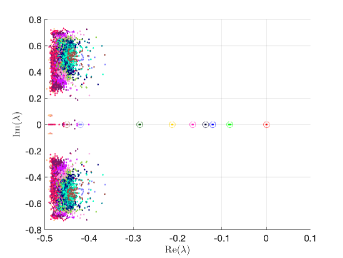
where and are the correlation lengths of the random variables , , in the and directions, respectively, and is the standard deviation of the Gaussian random field. The correlation lengths were set to be equal to of the width and height of the domain. The coefficient of variation of the lognormal field, defined as , where is the standard deviation and is the mean viscosity, was or . The viscosity (39) was parameterized using random variables. According to [21], in order to guarantee a complete representation of the lognormal process by (39), the degree of polynomial expansion of should be twice the degree of the expansion of the solution. We followed the same strategy here. Therefore, the values of and are, cf., e.g. [12, p. 87] or [33, Section 5.2], , . For the gPC expansion of eigenvalues/eigenvectors (11), the maximal degree of gPC expansion is , so then and . We used samples for the Monte Carlo method and Smolyak sparse grid with Gauss-Hermite quadrature points and grid level for collocation see, e.g., [17] for discussion of quadrature rules. With these settings, the size of in (16) was with nonzeros, and there were points in the sparse grid. As a consequence, the size of the stochastic Galerkin matrices is , the matrix associated with the Jacobian is fully block dense and the mass matrix is block diagonal, but we note that these matrices are never formed in implementation. For the solution of the Navier–Stokes problem we used the hybrid strategy with steps of Picard iteration followed by at most steps of Newton iteration. We used mean viscosity , which corresponds to Reynolds number , and the rightmost eigenvalue pair is , see the left panel in Figure 1. The Figure 3 displays Monte Carlo realizations of the eigenvalues with the largest real part for the values and . It can be seen that the rightmost eigenvalue is relatively less sensitive to perturbation comparing to the other eigenvalues, and since its real part is well separated from the rest of the spectrum, it can be easily identified in all runs of a sampling method. Figure 4 displays the probability density function (pdf) estimates of the rightmost eigenvalue with the positive imaginary part obtained directly by Monte Carlo, the stochastic collocation and stochastic Galerkin methods, for which the estimates were obtained using Matlab function ksdensity (in 2D) for sampled gPC expansions. Figure 5 shows plots of the estimated pdf of the real part of the rightmost eigenvalue. In both figures we can see a good agreement of the plots in the left column corresponding to and in the right column corresponding to . In Table 1 we tabulate the coefficients of the gPC expansion of the rightmost eigenvalue with positive imaginary part computed using the stochastic collocation and Galerkin methods. A good agreement of coefficients can be seen, in particular for coefficients with value much larger than zero, specifically with and. Finally, in Table 2 we examine the inexact line-search Newton iteration from Algorithm 1. For the line-search method, we set for the backtracking and . The initial guess is set using the rightmost eigenvalue and corresponding eigenvector of the eigenvalue problem (28) concatenated by zeros. The nonlinear iteration terminates when the norm of the residual . The linear systems in Line 4 of Algorithm 1 are solved using GMRES with the mean-based preconditioner (Algorithm 2), constraint mean-based preconditioner (Algorithm 3) and its updated variant discussed in Section 5.2.1, and the constraint hierarchical Gauss-Seidel preconditioner (Algorithm 4–5), which was used without truncation of the matrix-vector multiplications and also with truncation, setting , as discussed in Section 5.2. For the mean-based preconditioner we used , which worked best in our experience, and otherwise. For the constraint mean-based preconditioner the matrix from (35) was factored using LU decomposition, and the updated variant from Section 5.2.1 was used also in the constraint hierarchical Gauss-Seidel preconditioner. First, we note that the performance of the algorithm with the mean-based preconditioner was very sensitive to the choice of and , and it can be seen that it is quite sensitive also to . On the other hand, the performance of all variants of the constraint preconditioners appear to be far less sensitive, and we see only a mild increase in numbers of both nonlinear and GMRES iterations. Next, we see that updating the constraint mean-based preconditioner reduces the numbers of GMRES iterations in particular in the latter steps of the nonlinear method. Finally, we see that using the constraint hierarchical Gauss-Seidel preconditioner further decreases the number of GMRES iterations, for smaller it may be suitable to truncate the matrix-vector multiplications without any change in iteration counts and even though we see with an increase in number of nonlinear steps, the overall number of GMRES iterations remains smaller than when the two variants of the constraint mean-based preconditioner were used.
 |
 |
 |
 |
 |
 |
 |
 |
 |
 |
| SC | SG | ||
| 0 | 1 | 8.5726E-03 + 2.2551E+00 i | 8.5726E-03 + 2.2551E+00 i |
| 1 | 2 | -6.5686E-03 - 2.2643E-03 i | -6.5686E-03 - 2.2643E-03 i |
| 3 | 1.1181E-16 - 2.0817E-14 i | 2.6512E-17 + 8.3094E-17 i | |
| 2 | 4 | -1.1802E-06 - 2.4274E-05 i | -1.2055e-06 - 2.4200E-05 i |
| 5 | 3.8351E-15 - 4.4964E-15 i | 8.9732E-20 - 2.0565E-19 i | |
| 6 | -3.3393E-06 + 4.0603E-05 i | -3.3527E-06 + 4.0641E-05 i | |
| 3 | 7 | -1.0635E-07 + 4.1735E-07 i | -8.5671E-08 + 3.5926E-07 i |
| 8 | 7.8095E-16 + 6.1617E-15 i | -4.3191E-22 - 8.3970E-21 i | |
| 9 | -4.6791E-07 + 5.1602E-08 i | -4.4762E-07 - 6.0766E-09 i | |
| 10 | 2.2155E-15 + 4.6907E-15 i | 1.2691E-15 + 2.9181E-16 i | |
| 0 | 1 | 1.3420E-02 + 2.2577E+00 i | 1.3419E-02 + 2.2576E+00 i |
| 1 | 2 | -6.6200E-02 - 2.2034E-02 i | -6.6243E-02 - 2.2018E-02 i |
| 3 | 1.6011E-15 - 1.0297E-14 i | 1.1672E-15 + 8.8396E-16 i | |
| 2 | 4 | -2.2415E-04 - 2.5416E-03 i | -1.0889E-04 - 2.4178E-03 i |
| 5 | 8.5869E-17 - 1.0547E-15 i | 1.1865E-17 + 6.5559E-17 i | |
| 6 | -2.7323E-04 + 4.1219E-03 i | -2.1977E-04 + 4.1437E-03 i | |
| 3 | 7 | -4.8106E-05 + 3.556E-04 i | 1.3510E-04 + 9.1486E-05 i |
| 8 | 2.8365E-15 + 6.1062E-15 i | 8.0683E-19 + 5.3753E-18 i | |
| 9 | -4.5696E-04 + 2.7795E-06 i | -4.1149E-04 - 1.8160E-04 i | |
| 10 | 1.7408E-15 + 1.3101E-14 i | 1.3975E-15 + 3.5152E-16 i | |
| step | MB | cMB | cMBu | chGS | chGS2 | MB | cMB | cMBu | chGS | chGS2 |
|---|---|---|---|---|---|---|---|---|---|---|
| 1 | 2 | 1 | 1 | 1 | 1 | 7 | 1 | 1 | 1 | 1 |
| 2 | 2 | 1 | 1 | 1 | 1 | 6 | 3 | 2 | 3 | 3 |
| 3 | 6 | 3 | 2 | 1 | 1 | 13 | 4 | 4 | 3 | 4 |
| 4 | 9 | 6 | 3 | 2 | 2 | 10 | 8 | 7 | 3 | 4 |
| 5 | 15 | 10 | 6 | 3 | 3 | 15 | 16 | 13 | 4 | 5 |
| 6 | 14 | 8 | 8 | |||||||
| 7 | 25 | |||||||||
| 8 | 32 | |||||||||
| 9 | 67 | |||||||||
7.2 Expansion flow around a symmetric step
For the second example, we considered an expansion flow around a symmetric step. The domain and its discretization are shown in Figure 6. The spatial discretization used a uniform grid with QP-1 finite elements, which provided a stable discretization for the rectangular grid, see [8, p. 139]. There were velocity and pressure degrees of freedom. For the viscosity we considered a random field with affine dependence on the random variables given as
| (43) |
where is the mean and the standard deviation of the viscosity, , and with are the eigenpairs of the eigenvalue problem associated with the covariance kernel of the random field. As in the previous example, we used the values , and . We considered the same form of the covariance kernel as in (42),
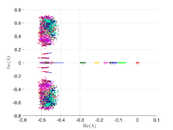
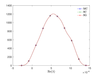
and the correlation lengths were set to of the width and of the height of the domain. We assume that the random variables follow a uniform distribution over . We note that (43) can be viewed as a special case of (39), which consists of only linear terms of. For the parametrization of viscosity by (43) we used the same stochastic dimension and degree of polynomial expansion as in the previous example: and , so then and . We used samples for the Monte Carlo method and Smolyak sparse grid with Gauss-Legendre quadrature points and grid level for collocation. With these settings, the size of in (16) was with nonzeros, and there were points on the sparse grid. As a consequence, the size of the stochastic Galerkin matrices is , and the matrix associated with the Jacobian has in this case a block-sparse structure see, e.g., [17, p. 88]. For the solution of the Navier–Stokes problem we used the hybrid strategy with steps of Picard iteration followed by at most steps of Newton iteration. We used mean viscosity , which corresponds to Reynolds number , and the rightmost eigenvalue is (the second largest eigenvalue is ), see the right panel in Figure 1. Figure 7 displays Monte Carlo realizations of the eigenvalues with the largest real part. As in the previous example, it can be seen that the rightmost eigenvalue is relatively less sensitive to perturbation comparing to the other eigenvalues, and it can be easily identified in all runs of a sampling method. Figure 8 displays the probability density function (pdf) estimates of the rightmost eigenvalue obtained directly by Monte Carlo, the stochastic collocation and stochastic Galerkin methods, for which the estimates were obtained using Matlab function ksdensity for sampled gPC expansions. We can see a good agreement of the plots in the left column corresponding to and in the right column corresponding to . In Table 3 we tabulate the coefficients of the gPC expansion of the rightmost eigenvalue computed using the stochastic collocation and stochastic Galerkin methods. A good agreement of coefficients can be seen, in particular for coefficients with larger values. Finally, we examine the inexact line-search Newton iteration from Algorithm 1. For the line-search method, we used the same setup as before with and . The initial guess is set using the rightmost eigenvalue and corresponding eigenvector of the eigenvalue problem (28), just with no imaginary part, concatenated by zeros. The nonlinear iteration terminates when the norm of the residual . The linear systems in Line 4 of Algorithm 1 are solved using right-preconditioned GMRES method as in the complex case. However, since the eigenvalue is real, the generalized eigenvalue problem as written in eq. (18) has the (usual) form given by eq. (9) and all algorithms formulated in this paper can be adapted by simply dropping the the components corresponding to the imaginary part of the eigenvalue problem: for example, the constraints mean-based preconditioner (Algorithm 3), and specifically (35) reduces to
and in the mean-based preconditioner (Algorithm 2) we also modified (32) as
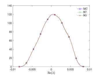
that is we used instead of in the shift of the matrix. We also adapted the constraint hierarchical Gauss-Seidel preconditioner (Algorithm 4–5), which was used as before without truncation of the matrix-vector multiplications and also with truncation, setting , as discussed in Section 5.2. For the mean-based preconditioner we used , but the preconditioner appeared to be far less sensitive to a specific value of, and otherwise. We note that this way the algorithms are still formulated for a generalized nonsymmetric eigenvalue problem unlike in [19], where we studied symmetric problems and in implementation we used a Cholesky factorization of the mass matrix in order to formulate a standard eigenvalue problem. From the results in Table 4 we see that for all preconditioners the overall number of nonlinear steps and GMRES iterations increases for larger , however all variants of the constraint preconditioner outperform the mean-based preconditioner the total number of iterations remains relatively small. Next, the performance with constraint preconditioners seem not improve with the updating discussed in Section 5.2.1, which is likely since the numbers of iterations are already low. Finally, using the constraint hierarchical Gauss-Seidel preconditioner reduces the number of GMRES iterations, which is slightly more significant for larger values of . The computational cost of preconditioner may be reduced by using the truncation of the matrix-vector multiplications; specifically we see that the overall iteration counts with and without the truncation are the same.

 |
 |
 |
 |
| SC | SG | SC | SG | ||
| 0 | 1 | 5.7873E-04 | 5.7873E-04 | 4.8948E-04 | 4.8927E-04 |
| 1 | 2 | -1.5948E-04 | -1.5948E-04 | -1.5890E-03 | -1.5877E-03 |
| 3 | -2.3689E-04 | -2.3689E-04 | -2.3619E-03 | -2.3605E-03 | |
| 2 | 4 | -2.4179E-07 | -2.6041E-07 | -2.4472E-05 | -2.6501E-05 |
| 5 | -8.2562E-07 | -8.7937E-07 | -8.3136E-05 | -8.8911E-05 | |
| 6 | -5.6059E-07 | -5.9203E-07 | -5.6429E-05 | -5.9831E-05 | |
| 3 | 7 | 7.7918E-10 | 8.2134E-10 | 5.7810E-07 | 8.5057E-07 |
| 8 | 2.5941E-09 | 3.9327E-09 | 2.8439E-06 | 4.022E-06 | |
| 9 | 3.8788E-09 | 5.5168E-09 | 4.0315E-06 | 5.6217E-06 | |
| 10 | 1.3002E-09 | 2.2685E-09 | 1.6668E-06 | 2.3171E-06 | |
| step | MB | cMB | cMBu | chGS | chGS2 | MB | cMB | cMBu | chGS | chGS2 |
|---|---|---|---|---|---|---|---|---|---|---|
| 1 | 19 | 4 | 4 | 2 | 2 | 23 | 6 | 6 | 3 | 3 |
| 2 | 17 | 4 | 4 | 3 | 3 | 20 | 6 | 6 | 4 | 4 |
| 3 | 15 | 3 | 3 | 3 | 3 | 19 | 6 | 6 | 4 | 4 |
| 4 | 15 | 5 | 5 | 4 | 4 | |||||
| 5 | 14 | 5 | 5 | 3 | 3 | |||||
| 6 | 23 | 8 | 8 | 5 | 5 | |||||
8 Conclusion
We studied inexact stochastic Galerkin methods for linear stability analysis of dynamical systems with parametric uncertainty and a specific application: the Navier–Stokes equation with stochastic viscosity. The model leads to a generalized eigenvalue problem with a symmetric mass matrix and nonsymmetric stiffness matrix, which was given by an affine expansion obtained from a stochastic expansion of the viscosity. For the assesment of linear stability we were interested in characterizing the rightmost eigenvalue using the generalized polynomial chaos expansion. Since the eigenvalue of interest may be complex, we considered separated representation of the real and imaginary parts of the associated eigenpair. The algorithms for solving the eigenvalue problem were formulated on the basis of line-search Newton iteration, in which the associated linear systems were solved using right-preconditioned GMRES method. We proposed several preconditioners: the mean-based preconditioner, the constraint mean-based preconditioner, and the constraint hierarchical Gauss-Seidel preconditioner. For the two constraint preconditioners we also proposed an updated version, which adapts the preconditioners to the linear system using Sherman-Morrison-Woodburry formula after each step of Newton iteration. We studied two model problems: one when the rightmost eigenvalue is given by a complex conjugate pair and another when the eigenvalue is real. The overall iteration count of GMRES with the constraint preconditioners was smaller compared to the mean-based preconditioner, and the constraint preconditioners were also less sensitive to the value of . Also we found that updating the constraint preconditioner after each step of Newton iteration and using the off-diagonal blocks in the action of the constraint hierarchical Gauss-Seidel preconditioner may further decrease the overall iteration count, in particular when the rightmost eigenvalue is complex. Finally, for both problems the probability density function estimates of the rightmost eigenvalue closely matched the estimates obtained using the stochastic collocation and also with the direct Monte Carlo simulation.
Acknowledgement
We would like to thank the anonymous reviewers for their insightful suggestions. Bedřich Sousedík would also like to thank Professors Pavel Burda, Howard Elman, Vladimír Janovský and Jaroslav Novotný for many discussions about bifurcation analysis and Navier–Stokes equations that inspired this work.
Appendix A Computations in inexact Newton iteration
The main component of a Krylov subspace method, such as GMRES, is the computation of a matrix-vector product. First, we note that the algorithms make use of the identity
| (44) |
Let us write a product with Jacobian matrix from (26) as
where
| (45) |
with , , , and , denoting the matrices in (22)–(25). Then, using (30) and (44), the matrix-vector product entails evaluating
| (46) | ||||
| (47) | ||||
| (48) | ||||
| (49) |
| (50) | ||||
| (51) |
and the right-hand side of (26) is evaluated using
and
where, using for either or , the th row of is
and the first term above is evaluated as
or, denoting the trace operator by, this term can be also evaluated as
Appendix B Parameters used in numerical experiments
In addition to the description in Section 7, we provide in Table 5 an overview of the main parameters used in the numerical experiments. Besides that, we used the following settings in both experiments. The gPC parameters: , , ; for the sampling methods: , ; for the inexact Newton iteration: , , stopping criterion ; for the preconditioners: (the mean-based preconditioner) and (otherwise).
| Section 7.1 | Section 7.2 | |
| problem | Flow around an obstacle | Expansion flow around a symmetric step |
| FEM | QQ1 | QP-1 |
| nelem// | 1008/8416/1096 | 976/8338/2928 |
| 373 | 220 | |
| 28 | 3 | |
| quadrature (in SC) | Gauss-Hermite | Gauss-Legendre |
| Solving the Navier–Stokes problem (see [30] for details): | ||
| max Picard steps | 6 | 20 |
| max Newton steps | 15 | 20 |
| nltol | ||
References
- [1] R. Andreev and C. Schwab. Sparse tensor approximation of parametric eigenvalue problems. In Numerical Analysis of Multiscale Problems, volume 83 of Lecture Notes in Computational Science and Engineering, pages 203–241, Berlin, Heidelberg, 2012. Springer.
- [2] Alex Bespalov, Daniel Loghin, and Rawin Youngnoi. Truncation preconditioners for stochastic galerkin finite element discretizations. SIAM Journal on Scientific Computing, pages S92–S116, 2021. (to appear).
- [3] K. A. Cliffe, T. J. Garratt, and A. Spence. Eigenvalues of block matrices arising from problems in fluid mechanics. SIAM Journal on Matrix Analysis and Applications, 15(4):1310–1318, 1994.
- [4] K. A. Cliffe, A. Spence, and S. J. Taverner. The numerical analysis of bifurcation problems with application to fluid mechanics. Acta Numerica, 9:39–131, 2000.
- [5] H. Elman and D. Silvester. Collocation methods for exploring perturbations in linear stability analysis. SIAM Journal on Scientific Computing, 40(4):A2667–A2693, 2018.
- [6] H. C. Elman, K. Meerbergen, A. Spence, and M. Wu. Lyapunov inverse iteration for identifying Hopf bifurcations in models of incompressible flow. SIAM Journal on Scientific Computing, 34(3):A1584–A1606, 2012.
- [7] H. C. Elman, A. Ramage, and D. J. Silvester. IFISS: A computational laboratory for investigating incompressible flow problems. SIAM Review, 56:261–273, 2014.
- [8] H. C. Elman, D. J. Silvester, and A. J. Wathen. Finite elements and fast iterative solvers: with applications in incompressible fluid dynamics. Numerical Mathematics and Scientific Computation. Oxford University Press, New York, second edition, 2014.
- [9] H. C. Elman and T. Su. Low-rank solution methods for stochastic eigenvalue problems. SIAM Journal on Scientific Computing, 41(4):A2657–A2680, 2019.
- [10] Oliver G. Ernst, Antje Mugler, Hans-Jörg Starkloff, and Elisabeth Ullmann. On the convergence of generalized polynomial chaos expansions. ESAIM: Mathematical Modelling and Numerical Analysis, 46(2):317–339, 2012.
- [11] R. G. Ghanem. The nonlinear Gaussian spectrum of log-normal stochastic processes and variables. Journal of Applied Mechanics, 66(4):964–973, 1999.
- [12] R. G. Ghanem and P. D. Spanos. Stochastic Finite Elements: A Spectral Approach. Springer-Verlag New York, Inc., New York, NY, USA, 1991. (Revised edition by Dover Publications, 2003).
- [13] W. Govaerts. Numerical Methods for Bifurcations of Dynamical Equilibria. SIAM, Philadelphia, 2000.
- [14] W. Hager. Updating the inverse of a matrix. SIAM Review, 31(2):221–239, 1989.
- [15] H. Hakula and M. Laaksonen. Multiparametric shell eigenvalue problems. Computer Methods in Applied Mechanics and Engineering, 343:721–745, 2019.
- [16] W. Kerner. Large-scale complex eigenvalue problems. Journal of Computational Physics, 85(1):1–85, 1989.
- [17] O. Le Maître and O. M. Knio. Spectral Methods for Uncertainty Quantification: With Applications to Computational Fluid Dynamics. Scientific Computation. Springer, 2010.
- [18] K. Lee, H. C. Elman, and B. Sousedík. A low-rank solver for the Navier-Stokes equations with uncertain viscosity. SIAM/ASA Journal on Uncertainty Quantification, 7(4):1275–1300, 2019.
- [19] K. Lee and B. Sousedík. Inexact methods for symmetric stochastic eigenvalue problems. SIAM/ASA Journal on Uncertainty Quantification, 6(4):1744–1776, 2018.
- [20] The Mathworks, Inc., Natick, Massachusetts. MATLAB version 9.10.0.1684407 (R2021a) Update 3, 2021.
- [21] H. G. Matthies and A. Keese. Galerkin methods for linear and nonlinear elliptic stochastic partial differential equations. Computer Methods in Applied Mechanics and Engineering, 194(12–16):1295–1331, 2005.
- [22] C. D. Meyer. Matrix Analysis and Applied Linear Algebra. Society for Industrial and Applied Mathematics, Philadelphia, PA, USA, 2000.
- [23] J. Nocedal and S. J. Wright. Numerical Optimization. Springer, New York, first edition, 1999.
- [24] C. E. Powell and D. J. Silvester. Preconditioning steady-state Navier-Stokes equations with random data. SIAM Journal on Scientific Computing, 34(5):A2482–A2506, 2012.
- [25] E. Sarrouy, O. Dessombz, and J.-J. Sinou. Stochastic analysis of the eigenvalue problem for mechanical systems using polynomial chaos expansion— application to a finite element rotor. Journal of Vibration and Acoustics, 134(5):1–12, 2012.
- [26] E. Sarrouy, O. Dessombz, and J.-J. Sinou. Piecewise polynomial chaos expansion with an application to brake squeal of a linear brake system. Journal of Sound and Vibration, 332(3):577–594, 2013.
- [27] P. J. Schmid and D. S. Henningson. Stability and Transition in Shear Flows. Springer, New York, 2001.
- [28] Benjamin E. Sonday, Robert D. Berry, Habib N. Najm, and Bert J. Debusschere. Eigenvalues of the Jacobian of a Galerkin-projected uncertain ode system. SIAM Journal on Scientific Computing, 33(3):1212–1233, 2011.
- [29] B. Sousedík and H. C. Elman. Inverse subspace iteration for spectral stochastic finite element methods. SIAM/ASA Journal on Uncertainty Quantification, 4(1):163–189, 2016.
- [30] B. Sousedík and H. C. Elman. Stochastic Galerkin methods for the steady-state Navier-Stokes equations. Journal of Computational Physics, 316:435–452, 2016.
- [31] B. Sousedík, H. C. Elman, K. Lee, and R. Price. On surrogate learning for linear stability assessment of Navier-Stokes equations with stochastic viscosity. Applications of Mathematics, 2022. (Accepted.) Preprint available at arXiv:2103.00622.
- [32] B. Sousedík and R. G. Ghanem. Truncated hierarchical preconditioning for the stochastic Galerkin FEM. International Journal for Uncertainty Quantification, 4(4):333–348, 2014.
- [33] D. Xiu. Numerical Methods for Stochastic Computations: A Spectral Method Approach. Princeton University Press, 2010.
- [34] D. Xiu and G. E. Karniadakis. The Wiener-Askey polynomial chaos for stochastic differential equations. SIAM Journal on Scientific Computing, 24(2):619–644, 2002.