Stochastic receding horizon control with output feedback and bounded control inputs
Abstract.
We provide a solution to the problem of receding horizon control for stochastic discrete-time systems with bounded control inputs and imperfect state measurements. For a suitable choice of control policies, we show that the finite-horizon optimization problem to be solved on-line is convex and successively feasible. Due to the inherent nonlinearity of the feedback loop, a slight extension of the Kalman filter is exploited to estimate the state optimally in mean-square sense. We show that the receding horizon implementation of the resulting control policies renders the state of the overall system mean-square bounded under mild assumptions. Finally, we discuss how some of the quantities required by the finite-horizon optimization problem can be computed off-line, reducing the on-line computation, and present some numerical examples.
Key words and phrases:
Predictive control, output feedback, constrained control, state estimation, stochastic controlEugenio.Cinquemani@inria.fr
1. Introduction
A considerable amount of research effort has been devoted to deterministic receding horizon control, see, for example, [Mayne et al., 2000; Bemporad and Morari, 1999; Lazar et al., 2007; Maciejowski, 2001; Qin and Badgwell, 2003] and references therein. Currently we have readily available conclusive proofs of successive feasibility and stability of receding horizon control laws in the noise-free deterministic setting. These techniques can be readily extended to the robust case, i.e., whenever there is an additive noise of bounded nature entering the system. The counterpart for stochastic systems subject to process noise and imperfect state measurements and bounded control inputs, however, is still missing. The principal obstacle is posed by the fact that it may not be possible to determine an a priori bound on the support of the noise, e.g., whenever the noise is additive and Gaussian. This extra ingredient complicates both the stability and feasibility proofs manifold: the noise eventually drives the state outside any bounded set no matter how large the latter is taken to be, and employing any standard linear state feedback means that any hard bounds on the control inputs will eventually be violated.
In this article we propose a solution to the general receding horizon control problem for linear systems with noisy process dynamics, imperfect state information, and bounded control inputs. Both the process and measurement noise sequences are assumed to enter the system in an additive fashion, and we require that the designed control policies satisfy hard bounds. Periodically at times , where is the control horizon, a certain finite-horizon optimal control problem is solved for a prediction horizon . The underlying cost is the standard expectation of the sum of cost-per-state functions that are quadratic in the state and control inputs [Bertsekas, 2005]. We also impose some variance-like bounds on the predicted future states and inputs—this is one possible way to impose soft state-constraints that are in spirit similar to integrated chance-constraints, e.g., in [Klein Haneveld, 1983; Klein Haneveld and van der Vlerk, 2006].
There are several key challenges that are inherent to our setup. First, since state-information is incomplete and corrupt, the need for a filter to estimate the state from the corrupt state measurements naturally presents itself. Second, it is clear that in the presence of unbounded (e.g., Gaussian) noise, it is not in general possible to ensure any bound on the control values with linear state feedback alone (assuming complete state information is available)—the additive nature of the noise ensures that the states exit from any fixed bounded set at some time almost surely. We see at once that nonlinear feedback is essential, and this issue is further complicated by the fact that only incomplete and imperfect state-information is available. Third, it is unclear whether applicatino of the control policies stabilizes the system in any reasonable sense.
In the backdrop of these challenges, let us mention the main contributions of this article. We
-
(i)
provide a tractable method for designing, in a receding horizon fashion, bounded causal nonlinear feedback policies, and
-
(ii)
guarantee that applying the designed control policies in a receding horizon fashion renders the state of the closed-loop system mean-square bounded for any initial state statistics.
We elaborate on the two points above:
-
(i)
Tractability: Given a subclass of causal policies, we demonstrate that the underlying optimal control problem translates to a convex optimization problem to be solved every time steps, that this optimization problem is feasible for any statistics of the initial state, and equivalent to a quadratic program. The subclass of polices we employ is comprised of open-loop terms and nonlinear feedback from the innovations. Under the assumption that the process and measurement noise is Gaussian, (even though the bounded inputs requirement makes the problem inherently nonlinear and it may appear that standard Kalman filtering may not apply,) it turns out that Kalman filtering techniques can indeed be utilized. We provide a low-complexity algorithm (essentially similar to standard Kalman filtering) for updating this conditional density, and report tractable solutions for the off-line computation of the time-dependent optimization parameters.
-
(ii)
Stability: It is well known that for noise-free discrete-time linear systems it is not possible to globally asymptotically stabilize the system, if the usual matrix has unstable eigenvalues, see, for example, [Yang et al., 1997] and references therein. Moreover, in the presence of stochastic process noise the hope for achieving asymptotic stability is obviously not realistic. Therefore, we naturally relax the notion of stability into mean-square boundedness of the state and impose the extra conditions that the system matrix is Lyapunov (or neutrally) stable and that the pair is stabilizable. Under such standard assumptions, we show that it is possible to augment the optimization problem with an extra stability constraint, and, consequently, that the successive application of our resulting policies renders the state of the overall system (plant and estimator) mean-square bounded.
Related Works
The research on stochastic receding horizon control is broadly subdivided into two parallel lines: the first treats multiplicative noise that enters the state equations, and the second caters to additive noise. The case of multiplicative noise has been treated in some detail in [Primbs, 2007; Primbs and Sung, 2009; Cannon et al., 2009], where the authors consider also soft constraints on the state and control input. However, in this article we exclusively focus on the case of additive noise.
The approach proposed in this article stems from and generalizes the idea of affine parametrization of control policies for finite-horizon linear quadratic problems proposed in [Ben-Tal et al., 2004, 2006], utilized within the robust MPC framework in [Ben-Tal et al., 2006; Löfberg, 2003; Goulart et al., 2006] for full state feedback, and in [van Hessem and Bosgra, 2003] for output feedback with Gaussian state and measurement noise inputs. More recently, this affine approximation was utilized in [Skaf and Boyd, 2009] for both the robust deterministic and the stochastic setups in the absence of control bounds, and optimality of the affine policies in the scalar deterministic case was reported in [Bertsimas et al., 2009]. In [Bertsimas and Brown, 2007] the authors reformulate the stochastic programming problem as a deterministic one with bounded noise and solve a robust optimization problem over a finite horizon, followed by estimating the performance when the noise can take unbounded values, i.e., when the noise is unbounded, but takes high values with low probability. Similar approach was utilized in [Oldewurtel et al., 2008] as well. There are also other approaches, e.g., those employing randomized algorithms as in [Batina, 2004; Blackmore and Williams, 2007; Maciejowski et al., 2005]. Results on obtaining lower bounds on the value functions of the stochastic optimization problem have been recently reported in [Wang and Boyd, 2009].
Organization
The remainder of this article is organized as follows. In Section 2 we formulate the receding horizon control problem with all the underlying assumptions, the construction of the estimator, and the main optimization problems to be solved. In Section 3 we provide the main results pertaining to tractability of the optimization problems and mean-square boundedness of the closed-loop system. We comment on the obtained results and provide some extensions in Section 4. We provide all the needed preliminary results, derivations, and proofs in Section 5, and some numerical examples in Section 6. Finally, we conclude in Section 7.
Notation
Let be a general probability space, we denote the conditional expectation given the sub- algebra of as . For any random vector we let . Hereafter we let and be the sets of positive and nonnegative integers, respectively. We let denote the trace of a square matrix, denote the standard norm, and simply denote the -norm. In a Euclidean space we denote by the closed Euclidean ball or radius centered at the origin. For any two matrices and of compatible dimensions, we denote by the -th step reachability matrix . For any matrix , we let and be its minimal and maximal singular values, respectively. We let denote the sub-matrix obtained by selecting the rows through of , and let denote its -th row.
2. Problem Setup
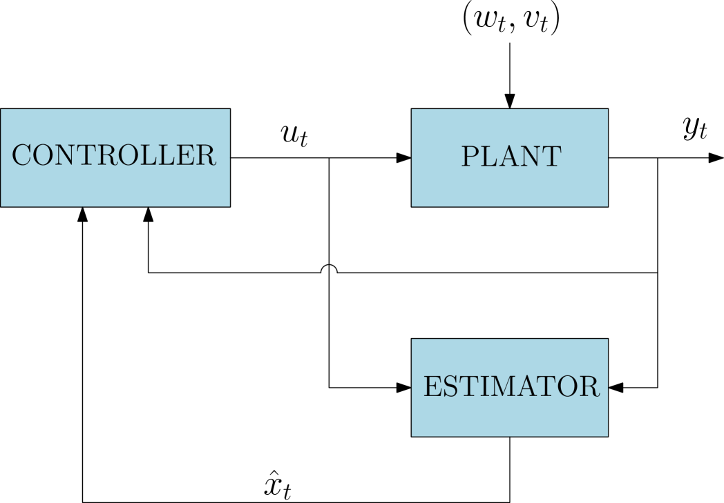
We are given a certain plant with discrete-time dynamics, process noise , and imperfect state measurements tainted through noise (Figure 1). The objective is to design a receding horizon controller which renders the overall closed-loop system mean-square bounded. We discuss the structure and the main assumptions on the dynamics of the system, the performance index to be minimized, and the construction of the optimal mean-square estimator in Subsection 2.1. Then, we formalize the optimization problem to be solved in a receding horizon fashion (to generate the input policies ) in Subsection 2.2.
2.1. Dynamics, Performance Index and Estimator
Consider the following affine discrete-time stochastic dynamical model:
| (2.1a) | ||||
| (2.1b) | ||||
where , is the state, is the control input, is the output, is a random process noise, is a random measurement noise, and , , and are known matrices. We posit the following main assumption:
Assumption 1.
- (i)
-
(ii)
The initial condition and the process and measurement noise vectors are normally distributed, i.e., , , and . Moreover, , and are mutually independent.
-
(iii)
The control inputs take values in the control constraint set:
(C1) i.e., for each .
Without any loss of generality, we also assume that is in real Jordan canonical form. Indeed, given a linear system described by system matrices , there exists a coordinate transformation in the state-space that brings the pair to the pair , where is in real Jordan form [Horn and Johnson, 1990, p. 150]. In particular, choosing a suitable ordering of the Jordan blocks, we can ensure that the pair has the form , where is Schur stable, and has its eigenvalues on the unit circle. By hypothesis (i)-(i)(b) of Assumption 1, is therefore block-diagonal with elements on the diagonal being either or rotation matrices. As a consequence, is orthogonal. Moreover, since is stabilizable, the pair must be reachable in a number of steps that depends on the dimension of and the structure of , i.e., . Summing up, we can start by considering that the state equation (2.1a) has the form
| (2.2) |
where is Schur stable, is orthogonal, and there exists a nonnegative integer such that the subsystem is reachable in steps. This integer is fixed throughout the rest of the article.
Fix a prediction horizon , and let us consider, at any time , the cost defined by:
| (2.3) |
where is the set of outputs up to time , (or more precisely the -algebra generated by the set of outputs,) and , , and are some given symmetric matrices of appropriate dimension, . At each time instant , we are interested in minimizing (2.3) over the class of causal output feedback strategies defined as:
| (2.4) |
for some measurable functions which satisfy the hard constraint (C1) on the inputs.
The cost in (2.3) is a conditional expectation given the observations up through time , and as such requires the conditional density of the state given the previous and current measurements. Our choice of causal control policies in (2.4) motivates us to rewrite the cost in (2.3) as:
| (2.5) |
The propagation of in time is not a trivial task in general. In what follows we shall report an iterative method for the computation of , whenever the control input is a measurable deterministic feedback from the past and present outputs. For , define and .
Assumption 2.
We require that and .
The following result is a slight extension of the usual Kalman Filter for which a proof can be found in Appendix A. An alternative proof can also be found in [Kumar and Varaiya, 1986, p.102].
Proposition 3.
In particular, the matrix together with characterize the conditional density , which is needed in the computation of the cost (2.5). Proposition 3 states that the conditional mean and covariances of can be propagated by an iterative algorithm which resembles the Kalman filter. Since the system is generally nonlinear due to the function being nonlinear, we cannot assume that the probability distributions in the problem are Gaussian (in fact, the a priori distributions of and of are not) and the proof cannot be developed in the standard linear framework of the Kalman filter.
Hereafter, we shall denote for notational convenience by the estimate , and let
| (2.10) |
which corresponds to the Jordan decomposition in (2.2).
2.2. Optimization Problem and Control Policies
Having discussed the iterative update of the laws of given the measurements in Section 2.1, we return to our optimization problem in (2.5). We can rewrite our optimization problem as:
| (OP1) |
where the collection of functions were defined following (2.4).
The explicit solution via dynamic programming to Problem (OP1) over the class of causal feedback policies , is difficult if not impossible to obtain in general [Bertsekas, 2000, 2007]. One way to circumvent this difficulty is to restrict our search for feedback policies to a subclass of . This will result in a suboptimal solution to our problem, but may yield a tractable optimization problem. This is the track we pursue next.
Given a control horizon and a prediction horizon , we would like to periodically solve Problem (OP1) at times over the following class of affine-like control policies
| (POL) |
where , and for any vector , , where is the -th element of the vector and is any function with . The feedback gains and the affine terms are the decision variables. The value of in (POL) depends on the values of the measured outputs from the beginning of the prediction horizon at time up to time only, which requires a finite amount of memory. Note that we have chosen to saturate the measurements we obtain from the vectors before inserting them into the control policy. This way we do not assume that either the process noise or the measurement noise distributions are defined over a compact domain, which is a crucial assumption in robust MPC approaches [Mayne et al., 2000]. Moreover, the choice of element-wise saturation functions is left open. As such, we can accommodate standard saturation, piecewise linear, and sigmoidal functions, to name a few.
Finally, we collect all the ingredients of the stochastic receding horizon control problem in Algorithm 1 below.
Compact Notation
In order to state the main results in Section 3, it is convenient to utilize a more compact notation that describes the evolution of all signals over the entire prediction horizon .
The evolution of the system dynamics (2.1a)-(2.1b) over a single prediction horizon , starting at , can be described in a lifted form as follows:
| (2.11) | ||||
where , , , , , ,
and . Let
be the usual Kalman gain and define , and . Then, we can write the estimation error vector as
| (2.12) |
where , ,
Finally, the innovations sequence can be written as
| (2.13) |
where . Consequently, the innovations sequence over the prediction horizon is independent of the inputs vector .
The cost function (2.3) at time can be written as
| (2.14) |
where and . Also, the control policy (POL) at time is given by
| (POL) |
where
and has the following lower block diagonal structure
| (2.15) |
Since the innovation vector in (2.13) is not a function of and , the control inputs in (POL) remain affine in the decision variables. This fact is important to show convexity of the optimization problem, as will be seen in the next section. Finally, the constraint (C1) can be rewritten as:
| (C1) |
3. Main Results
The optimization problem (OP1) we have stated so far, even if it is successively feasible, does not in general guarantee stability of the resulting receding horizon controller in Algorithm 1. Unlike deterministic stability arguments utilized in MPC (see, for example, [Mayne et al., 2000]), we cannot assume the existence of a final region that is control positively invariant and which is crucial to establish stability. This is simply due to the fact that the process noise sequence is not assumed to have a compact domain of support. However, guided by our earlier results in [Ramponi et al., 2009], we shall enforce an extra stability constraint which, if feasible, can render the state of the closed-loop system mean-square bounded.
For , the state estimate at time given the state estimate at time , the control inputs from time through , and the corresponding process and measurement noise sequences can be written as
where we define
| (3.1) | ||||
Scholium 4.
There exists an integer and a positive constant such that
| (3.2) |
A proof of Scholium 4 appears in Section 5. Using the constant , we now require the following “drift condition” to be satisfied: for any given and for every , there exists a , such that the following condition is satisfied
| (C2) |
Note that . (For notational convenience, we have retained with the knowledge that the matrix causally selects the outputs as they become available, see (2.15).) The constraint (C2) pertains only to the second subsystem of the estimator, as the first subsystem () is Schur stable (see (2.2) and (2.10)). We augment problem (OP1) with the stability constraint (C2) to obtain
| (OP2) |
Assumption 5.
Theorem 6 (Main Result).
Consider the system (2.1a)-(2.1b), and suppose that Assumption 5 holds. Then:
-
(i)
For every time , the optimization problem (OP2) is convex, feasible, and can be approximated to the following quadratic optimization problem:
(3.3) subject to (3.4) (3.5) where ,
(3.6) -
(ii)
For every initial state and noise statistics , successive application of the control laws given by the optimization problem in (i) for steps renders the closed-loop system mean-square bounded in the following sense: there exists a constant such that
(3.7)
In practice, it may be also of interest to impose further some soft constraints both on the state and the input vectors. For example, one may be interested in imposing quadratic or linear constraints on the state, both of which can be captured in the following
| (C3) |
where and . Moreover, expected energy expenditure constraints can be posed as follows
| (C4) |
where and . In the absence of hard input constraints, such expectation-type constraints are commonly used in the stochastic MPC [Primbs and Sung, 2009; Agarwal et al., 2009] and in stochastic optimization in the form of integrated chance constraints [Klein Haneveld, 1983; Klein Haneveld and van der Vlerk, 2006]. This is partly because it is not possible, without posing further restrictions on the boundedness of the process noise , to ensure that hard constraints on the state are satisfied. For example, in the standard LQG setting nontrivial hard constraints on the system state would generally be violated with nonzero probability. Moreover, in contrast to chance constraints where a bound is imposed on the probability of constraint violation, expectation-type constraints tend to give rise to convex optimization problems under weak assumptions [Agarwal et al., 2009].
We can also augment problem (OP2) with the constraints (C3) and (C4) to obtain
| (OP3) |
Notice that the constraints (C3) and (C4) are not necessarily feasible at time for any choice of parameters and . As such, problem (OP3) may become infeasible over time if we simply apply Algorithm 1. We therefore replace the optimization Step 7 in Algorithm 1 with the following subroutine for some given and that make the constraints feasible, precision number and maximal number of iterations :
Subroutine 7
-
7a:
Set , , , and
-
7b:
Solve the optimization problem (OP3) using and to obtain the sequence
-
7c:
Set
-
7d:
repeat
-
7e:
Set and
-
7f:
Solve Solve the optimization problem (OP3) using the new and to obtain
the sequence -
7g:
if step 5f is feasible then
-
7h:
Set and
-
7i:
Set
-
7j:
else
-
7k:
Set and
-
7l:
end if
-
7m:
set
-
7n:
until ( and ) or
It may be argued that replacing Step 7 in Algorithm 1 with Subroutine 7 above increases the computational burden; however, the parameter guarantees that this iterative process is halted after some prespecified number of steps in case the required precision is not reached in the meantime. In some instances, we may be given some fixed parameters and with which the constraints (C3) and (C4) have to be satisfied, respectively. This requirement can be easily incorporated into Subroutine 7 by setting and in step 7a.
Assumption 7.
At each time step , the constants and in Subroutine 7 are chosen as
Corollary 8.
Consider the system (2.1a)-(2.1b), and suppose that Assumption 5, and 7 hold. Then:
-
(i)
For every time the optimization problem (OP3) solved in Subroutine 7 is convex, feasible, and equivalent to the following quadratically constrained quadratic optimization problem:
(3.8) (3.9) -
(ii)
For every initial state and noise statistics , successive application of the control laws given by the optimization problem in (i) for steps renders the closed-loop system mean-square bounded in the following sense: there exists a constant such that
4. Discussion
The optimization problem (OP2) being solved in Theorem 6 is a quadratic program (QP), whereas the optimization problem (OP3) being solved in Corollary (8) is a quadratically constrained quadratic program (QCQP) in the optimization parameters . As such, both can be easily solved via software packages such as cvx [Grant and Boyd, 2000] or yalmip [Löfberg, 2004].
4.1. Other Constraints and Policies
It is not difficult to see that constraints on the variation of the inputs of the form
where , can be incorporated into the optimization problems (OP2) and (OP3). Moreover, we can easily solve the problem using quadratic policies of the form
| (POL′) |
instead of (POL), where
and . The underlying optimization problems (OP2) and (OP3) with the policy (POL′) are still convex and both Theorem (6) and Corollary (8) still apply with minor changes.
4.2. Off-Line Computation of the Matrices
At any time , our ability to solve the optimization problems (OP2) and (OP3) in Theorem 6 and Corollary 8, respectively, hinges upon our ability to compute the following matrices
| (4.1) | ||||||
Recall that is the innovations sequence that was given in (2.13), and is the optimal mean-square estimate of given the history . The matrices (4.1) may be computed by numerical integration with respect to the independent Gaussian measures of , of , and of given . Due to the large dimensionality of the integration space, this approach may be impractical for online computations. One alternative approach relies on the observation that , and depend on via the difference . Since is conditionally zero-mean given , we can write the dependency of (4.1) on the time-varying statistics of given as follows:
| (4.2) | ||||
In principle one may compute off-line and store the matrices , and , which depend on the covariance matrices , and just update online the value of as the estimate becomes available. However, this poses serious requirements in terms of memory. A more appealing alternative is to exploit the convergence properties of . The following result can be inferred, for instance, from [Kamen and Su, 1999, Theorem 5.1].
Proposition 9.
The assumption that can be relaxed to at the price of some additional technicality (more on this can be found in [Ferrante et al., 2002]). As a consequence of this result, under detectability and stabilizability assumptions, converges to
| (4.4) |
which is the asymptotic error covariance matrix of the estimator . Thus, neglecting the initial transient, it makes sense to just compute off-line and store the matrices , and , and just update the matrix for new values of the estimate .
5. Proofs
The proofs of the main results are presented as follows: We begin by showing the result in Scholium 4. Then, we state a fundamental result pertaining to mean-square boundedness for general random sequences in Proposition 11, which is utilized to show the mean-square boundedness conclusions of Theorem 6 and Corollary 8. We proceed to show the first assertion (i) of Theorem 6 in Lemma 12. The proof of the second assertion (ii) of Theorem 6 starts by showing Lemmas 13 and 14 to conclude mean-square boundedness of the orthogonal subsystem . We conclude the proof of Theorem 6 by showing mean-square boundedness of the Schur stable subsystem . We end this section by proving the extra conclusions of Corollary 8, beyond those present in Theorem 6.
Let us now look at the estimation equation in (2.6) and combine it with (2.8) and the output equation (2.1b) to obtain
| (5.1) |
where is the Kalman gain. Our next Fact pertains to the boundedness of the error covariance matrices in (2.7).
Fact 10.
There exists and such that for all , and for all .
Fact 10 follows, for example, immediately from Lemma 15 in Appendix B and since by assumption , one possible bound on is given by . Note that there are many alternative bounds in the Literature, see, for example, [Anderson and Moore, 1979; Jazwinski, 1970]. Now, using the bounds in Fact 10, we can proceed to prove Scholium 4.
Proof of Scholium 4.
Recall the expression of in (3.1) and define the following quantities:
| (5.2) | ||||
Then, can be rewritten as
| (5.3) |
But for , 111Recall that for any positive real number , denotes the smallest integer that upper-bounds . we have that
Using Fact 10 we know that . Thus, it suffices to take
in order to upper-bound the expectation of in (5.3) after time . ∎
The following result pertains to mean-square boundedness of a random sequence :
Proposition 11 ([Pemantle and Rosenthal, 1999, Theorem 1]).
Let be a sequence of nonnegative random variables on some probability space , and let be any filtration to which is adapted. Suppose that there exist constants , and , such that
and for all :
| (5.4) | |||
| (5.5) |
Then there exists a constant such that .
Lemma 12.
Proof.
It is clear that is convex quadratic in and , and both and are affine functions of the design parameters for every realization of the noise . Since taking expectation of a convex function retains convexity [Boyd and Vandenberghe, 2004], we conclude that is convex in . Also, note that the constraint sets described by (3.4) and (3.5) are convex in . This settles the claim concerning convexity of the optimization program in Theorem 6-(i).
Concerning the objective function (3.3), we have that
Since and in view of the definitions of the various matrices in (3.6) we have
This tallies the objective function in (3.3) with the objective in (2.14).
Concerning the constraints, we have shown in [Hokayem et al., 2009; Chatterjee et al., 2009] that combining the constraint and the class of policies (POL) is equivalent to the constraints for all , which accounts for the constraint (3.4). Substituting (POL) into the stability constraint (C2), we obtain
Accordingly, if condition constraint (3.5) is satisfied, then the stability constraint (C2) is satisfied as well.
It remains to show that the constraints are simultaneously feasible. Inspired by the work in [Ramponi et al., 2009], we consider the candidate controller
i.e., with , where . First, we have that
and the constraint (C1) is satisfied. Concerning constraint (C2), we have that
| (5.6) |
where the first equality follows from the orthogonality of (see [Ramponi et al., 2009]), and the constraint (3.5) is also satisfied. The optimization program (3.3) subject to (3.4)-(3.5) is therefore a quadratic program that is equivalent to (OP2). ∎
Lemma 13.
Proof.
Let be a projection operator that picks the last components of any vector in , and consider the subsampled process given by
| (5.7) |
By utilizing the triangle inequality we get
We know from Scholium 4 that there exists a uniform (with respect to time ) upper bound for the last term on the right-hand side of the preceding inequality for . We rewrite the inequality as
where the last inequality follows from (5.6). Setting and completes the proof. ∎
Lemma 14.
Proof.
Fix , and consider again the subsampled process in (5.7). We have, by orthogonality of , that and, by the triangle inequality, that
Recall that for any two positive numbers and , . Using this latter fact, we arrive at the following upper bound
By design and is Gaussian and independent of and has its fourth moment bounded. Therefore, we can easily infer that there exists an such that
for all . ∎
We are finally ready to prove Theorem 6.
Proof of Theorem 6.
Claim (i) of Theorem 6 was proved in Lemma 12. It remains to show claim (ii). We start by asserting the following inequality
We know from Fact 10 that for all . As such, if we are able to show that the state of the estimator is mean-square bounded, we can immediately infer a mean-square bound on the state of the plant.
We first start by splitting the squared norm of the estimator state as , where and are states corresponding to the Schur and orthogonal parts of the system, respectively. It then follows that
| (5.8) |
Letting for , we see from Lemma 13 and Lemma 14 the conditions (5.4) and (5.5) of Proposition 11 are verified for the sequence . Thus, by Proposition 11, there exists a constant such that
Hence, the orthogonal subsystem is mean-square bounded.
Since the matrix is Schur stable, we know [Bernstein, 2009, Proposition 11.10.5] that there exists a positive definite matrix that satisfies . It easily follows that there exists such that ; in fact, can be chosen from the interval . Therefore, we see that for any ,
where is the projection onto the first coordinates and was defined in (3.1). Young’s inequality shows that for . Choosing and utilizing Fact 10 and the upper bound on the inputs , it follows that for all ,
Therefore, for , we have that
Iterating the last inequality, it follows that
or
We can conclude that there exists such that
| (5.9) |
We can therefore conclude that
Since the sequence in (2.1a) is generated through the addition of independent mean-square bounded random variables and a bounded control input, and since , it follows that there exists such that
Proof of Corollary 8.
The proof of Corollary 8 follows exactly the same reasoning as in the proof of Theorem 6, up to the constraints in (3.8) and (3.9). Also, rewriting the constraints (C3) and (C4) as (3.8) and (3.9), respectively, can be done similarly to the way we rewrote the cost in Theorem (6). It remains to show the upper bounds and in Assumption (7).
The constraint (C3) can be upper-bounded as follows:
where the first inequality follows from the fact that , for any , and the noise being zero-mean, the second inequality follows from applying norm bounds between the 2 and -norms and Hölder’s inequality. As for the constraint (C4), it can be upper-bounded as follows:
This completes the proof. ∎
6. Examples
Consider the system (2.1a)-(2.1b) with the following matrices:
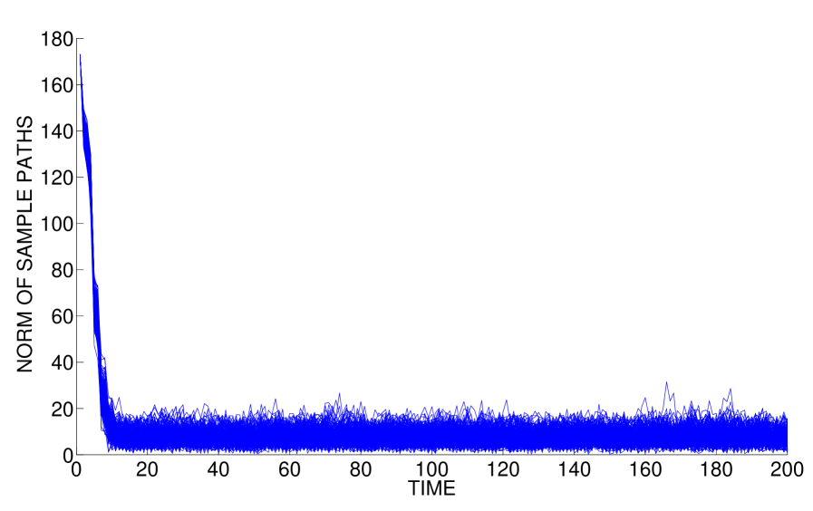
The simulation data was chosen to be , , , , , , , and the usual piecewise linear saturation function with . For this example the theoretical bound on the input is for a choice of .
We simulated the system for the discrete-time interval using Algorithm 1, without the constraints (C3) and (C4). The coding was done using MATLAB and the optimization problem was solved using yalmip [Löfberg, 2004] and sdpt3 [Toh et al., 1999]. The computation of the matrices , , , and was done off-line using the steady state error covariance matrix , as discussed in the previous section, via classical Monte Carlo integration [Robert and Casella, 2004, Section 3.2] using samples.
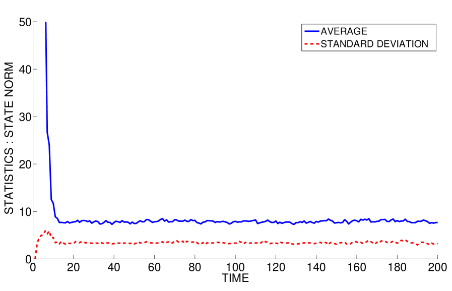
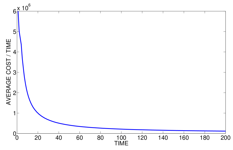
The norms of the state trajectories for 200 different sample paths of the process and measurement noises are plotted in Figure 2 starting from . The average state norm as well as the standard deviation of the state norm are depicted in Figure 3, where it is clear that the proposed controller renders the system mean-square bounded. The average total cost normalized by time for this simulation is plotted in Figure 4.
7. Conclusions
We presented a method for stochastic receding horizon control of discrete-time linear systems with process and measurement noise and bounded input policies. We showed that the optimization problem solved periodically is successively feasible and convex. Moreover, we illustrated how a certain stability condition can be utilized to show that the application of the receding horizon controller renders the state of the system mean-square bounded. We discussed how certain matrices in the cost function can be computed off-line and provided an example that illustrates our approach.
References
- Agarwal et al. [2009] Agarwal, M., Cinquemani, E., Chatterjee, D., Lygeros, J., 2009. On convexity of stochastic optimization problems with constraints. In: European Control Conference. pp. 2827–2832.
- Anderson and Moore [1979] Anderson, B., Moore, J., 1979. Optimal Filtering. Prentice-Hall.
- Batina [2004] Batina, I., 2004. Model predictive control for stochastic systems by randomized algorithms. Ph.D. thesis, Technische Universiteit Eindhoven.
- Bemporad and Morari [1999] Bemporad, A., Morari, M., 1999. Robust model predictive control: a survey. Robustness in Identification and Control 245, 207–226.
- Ben-Tal et al. [2006] Ben-Tal, A., Boyd, S., Nemirovski, A., 2006. Extending scope of robust optimization: Comprehensive robust counterparts of uncertain problems. Journal of Mathematical Programming 107, 63–89.
- Ben-Tal et al. [2004] Ben-Tal, A., Goryashko, A., Guslitzer, E., Nemirovski, A., 2004. Adjustable robust solutions of uncertain linear programs. Mathematical Programming 99 (2), 351–376.
- Bernstein [2009] Bernstein, D. S., 2009. Matrix Mathematics, 2nd Edition. Princeton University Press.
- Bertsekas [2000] Bertsekas, D. P., 2000. Dynamic Programming and Optimal Control, 2nd Edition. Vol. 1. Athena Scientific.
- Bertsekas [2005] Bertsekas, D. P., 2005. Dynamic programming and suboptimal control: a survey from ADP to MPC. European Journal of Control 11 (4-5).
- Bertsekas [2007] Bertsekas, D. P., 2007. Dynamic Programming and Optimal Control, 3rd Edition. Vol. 2. Athena Scientific.
- Bertsimas and Brown [2007] Bertsimas, D., Brown, D. B., 2007. Constrained stochastic LQC: a tractable approach. IEEE Transactions on Automatic Control 52 (10), 1826–1841.
- Bertsimas et al. [2009] Bertsimas, D., Iancu, D. A., Parrilo, P. A., 2009. Optimality of affine policies in multi-stage robust optimizationPreprint available at: http://arxiv.org/abs/0904.3986.
- Blackmore and Williams [2007] Blackmore, L., Williams, B. C., July 2007. Optimal, robust predictive control of nonlinear systems under probabilistic uncertainty using particles. In: Proceedings of the American Control Conference. pp. 1759 – 1761.
- Boyd and Vandenberghe [2004] Boyd, S., Vandenberghe, L., 2004. Convex Optimization. Cambridge University Press, Cambridge, sixth printing with corrections, 2008.
- Cannon et al. [2009] Cannon, M., Kouvaritakis, B., Wu, X., July 2009. Probabilistic constrained MPC for systems with multiplicative and additive stochastic uncertainty. IEEE Transactions on Automatic Control 54 (7), 1626–1632.
- Chatterjee et al. [2009] Chatterjee, D., Hokayem, P., Lygeros, J., 2009. Stochastic receding horizon control with bounded control inputs: a vector space approach. IEEE Transactions on Automatic ControlUnder review. http://arxiv.org/abs/0903.5444.
- Ferrante et al. [2002] Ferrante, A., Picci, G., Pinzoni, S., 2002. Silverman algorithm and the structure of discrete-time stochastic systems. Linear Algebra and its Applications 351/352, 219–242.
- Goulart et al. [2006] Goulart, P. J., Kerrigan, E. C., Maciejowski, J. M., 2006. Optimization over state feedback policies for robust control with constraints. Automatica 42 (4), 523–533.
- Grant and Boyd [2000] Grant, M., Boyd, S., December 2000. CVX: Matlab software for disciplined convex programming (web page and software). http://stanford.edu/~boyd/cvx.
- Hokayem et al. [2009] Hokayem, P., Chatterjee, D., Lygeros, J., 2009. On stochastic model predictive control with bounded control inputs. In: Proceedings of the combined 48th IEEE Conference on Decision & Control and 28th Chinese Control Conference. pp. 6359–6364, available at http://arxiv.org/abs/0902.3944.
- Horn and Johnson [1990] Horn, R. A., Johnson, C. R., 1990. Matrix Analysis. Cambridge University Press, Cambridge.
- Jazwinski [1970] Jazwinski, A. H., 1970. Stochastic Processes and Filtering Theory. Academic Press.
- Kamen and Su [1999] Kamen, E. W., Su, J. K., 1999. Introduction to Optimal Estimation. Springer, London, UK.
- Klein Haneveld [1983] Klein Haneveld, W. K., 1983. On integrated chance constraints. In: Stochastic programming (Gargnano). Vol. 76 of Lecture Notes in Control and Inform. Sci. Springer, Berlin, pp. 194–209.
- Klein Haneveld and van der Vlerk [2006] Klein Haneveld, W. K., van der Vlerk, M. H., 2006. Integrated chance constraints: reduced forms and an algorithm. Computational Management Science 3 (4), 245–269.
- Kumar and Varaiya [1986] Kumar, P. R., Varaiya, P., 1986. Stochastic Systems: Estimation, Identification, and Adaptive Control. Prentice Hall.
- Lazar et al. [2007] Lazar, M., Heemels, W. P. M. H., Bemporad, A., Weiland, S., 2007. Discrete-time non-smooth nonlinear MPC: stability and robustness. In: Lecture Notes in Control and Information Sciences. Vol. 358. Springer-Verlag, pp. 93–103.
- Löfberg [2003] Löfberg, J., 2003. Minimax Approaches to Robust Model Predictive Control. Ph.D. thesis, Linköpings Universitet.
- Löfberg [2004] Löfberg, J., 2004. YALMIP : A Toolbox for Modeling and Optimization in MATLAB. In: Proceedings of the CACSD Conference. Taipei, Taiwan.
- Maciejowski [2001] Maciejowski, J. M., 2001. Predictive Control with Constraints. Prentice Hall.
- Maciejowski et al. [2005] Maciejowski, M., Lecchini, A., Lygeros, J., 2005. NMPC for complex stochastic systems using Markov Chain Monte Carlo. Vol. 358/2007 of Lecture Notes in Control and Information Sciences. Springer, Stuttgart, Germany, pp. 269–281.
- Mayne et al. [2000] Mayne, D. Q., Rawlings, J. B., Rao, C. V., Scokaert, P. O. M., Jun 2000. Constrained model predictive control: stability and optimality. Automatica 36 (6), 789–814.
- Oldewurtel et al. [2008] Oldewurtel, F., Jones, C., Morari, M., Dec 2008. A tractable approximation of chance constrained stochastic MPC based on affine disturbance feedback. In: Conference on Decision and Control, CDC. Cancun, Mexico.
- Pemantle and Rosenthal [1999] Pemantle, R., Rosenthal, J. S., 1999. Moment conditions for a sequence with negative drift to be uniformly bounded in . Stochastic Processes and their Applications 82 (1), 143–155.
- Primbs [2007] Primbs, J., 2007. A soft constraint approach to stochastic receding horizon control. In: Proceedings of the 46th IEEE Conference on Decision and Control. pp. 4797 – 4802.
- Primbs and Sung [2009] Primbs, J. A., Sung, C. H., Feb. 2009. Stochastic receding horizon control of constrained linear systems with state and control multiplicative noise. IEEE Transactions on Automatic Control 54 (2), 221–230.
- Qin and Badgwell [2003] Qin, S. J., Badgwell, T., Jul. 2003. A survey of industrial model predictive control technology. Control Engineering Practice 11 (7), 733–764.
- Ramponi et al. [2009] Ramponi, F., Chatterjee, D., Milias-Argeitis, A., Hokayem, P., Lygeros, J., 2009. Attaining mean square boundedness of a marginally stable noisy linear system with a bounded control input. http://arxiv.org/abs/0907.1436, submitted to IEEE Transactionson Automatic Control, Revised Jan 2010.
- Robert and Casella [2004] Robert, C. P., Casella, G., 2004. Monte Carlo Statistical Methods, 2nd Edition. Springer.
- Skaf and Boyd [2009] Skaf, J., Boyd, S., 2009. Design of affine controllers via convex optimization. http://www.stanford.edu/~boyd/papers/affine_contr.html.
- Toh et al. [1999] Toh, K., Todd, M., Tatuncu, R., 1999. SDPT3– a Matlab software package for semidefinite programming. Optimization Methods and Software (11), 545–581, http://www.math.nus.edu.sg/~mattohkc/sdpt3.html.
- van Hessem and Bosgra [2003] van Hessem, D. H., Bosgra, O. H., 2003. A full solution to the constrained stochastic closed-loop MPC problem via state and innovations feedback and its receding horizon implementation. In: Proceedings of the 42nd IEEE Conference on Decision and Control. Vol. 1. pp. 929–934.
- Wang and Boyd [2009] Wang, Y., Boyd, S., 2009. Peformance bounds for linear stochastic control. Systems and Control Letters 58 (3), 178–182.
- Yang et al. [1997] Yang, Y. D., Sontag, E. D., Sussmann, H. J., 1997. Global stabilization of linear discrete-time systems with bounded feedback. Systems and Control Letters 30 (5), 273–281.
Appendix A Proof of Proposition 3
For , , with , by assumption. Assume now that, for a given , is normal with mean and covariance matrix . By Assumption 1-(ii) and dynamics in (2.1b), is also normal with mean and covariance matrix . Hence, applying Bayes rule we may write
where we have by the Chapman-Kolmogorov equation. It follows that
where the proportionality constants do not depend on . Let us now focus on the term within square brackets and write , , and in place of , , and for shortness. Expanding the products and collecting the linear and quadratic terms in one gets
Since and by assumption, it follows that . If we let , the expression above can be rewritten as
Completing the square, the latter expression becomes
where depends on and but not on . Factoring out of the two terms and simplifying yields
Hence,
with , where the missing normalization constant does not depend on . Hence, is normal with mean and covariance matrix . Using the matrix inversion lemma, , which is (2.7). To obtain (2.6), replace by in the expression of to get
Finally, using the identity (where the inverse exists because and ) and the definition of ,
which leads to (2.6).
To conclude the proof, we need to compute the density and prove (2.8)–(2.9). Using the Chapman-Kolmogorov equation, we can compute the density as follows
| (A.1) |
However, the explicit computation of the integral in (A.1) is a very tedious exercise. We shall instead rely on characteristic functions. Recall that the characteristic function of an -dimensional Gaussian random vector with mean and covariance is given by , where and . The characteristic function of given is then
where we have used system dynamics in (2.1a) and the general definition of the feedback policies (2.4). Since is independent of and and it is Gaussian with mean and covariance , . Therefore the last expression in the chain becomes
It was proved above that, conditionally on , is Gaussian with mean and covariance matrix . Hence
and consequently
which is the characteristic function of a Gaussian random vector with mean and covariance matrix .
Appendix B
Lemma 15.
Proof.
First, observe that
and since is controllable by Assumption 5-(iii), we see that there exists such that for all the rank of ; indeed, is the reachability index of . Thus, is positive definite, and therefore, there exists some such that
| (B.2) |
Second, observe that333Here denotes the standard Kronecker product.
Since is observable by assumption, there exists such that the rank of the matrix is . The matrix is clearly positive definite by Assumption 5’(iii), and therefore, we see that there exists such that