Stochastic resetting on comb-like structures***V. D. and A. M. contributed equally to this work.
Abstract
We study a diffusion process on a three-dimensional comb under stochastic resetting. We consider three different types of resetting: global resetting from any point in the comb to the initial position, resetting from a finger to the corresponding backbone and resetting from secondary fingers to the main fingers. The transient dynamics along the backbone in all three cases is different due to the different resetting mechanisms, finding a wide range of dynamics for the mean squared displacement. For the particular geometry studied herein, we compute the stationary solution and the mean square displacement and find that the global resetting breaks the transport in the three directions. Regarding the resetting to the backbone, the transport is broken in two directions but it is enhanced in the main axis. Finally, the resetting to the fingers enhances the transport in the backbone and the main fingers but reaches a steady value for the mean squared displacement in the secondary fingers.
pacs:
87.19.L-, 05.40.Fb, 82.40.-gI Introduction
Combs are two- or three-dimensional branched structures with a backbone crossed by perpendicular fingers. These fingers may be one or two dimensional side structures. A random walker moving along the backbone may enter into a finger (or fingers) and move there for a time and return to the backbone to start the process again. As a result of a Brownian motion in a two-dimensional comb the mean squared displacement (MSD) shows a subdiffusive behavior depending on time as and was originally introduced to understand anomalous transport in percolation clusters and many other applications book . Although three-dimensional combs have been less developed, they have modeled transport in spiny dendrites MeIo13 or ultraslow diffusion in combs with circular fingers IoMe16 .
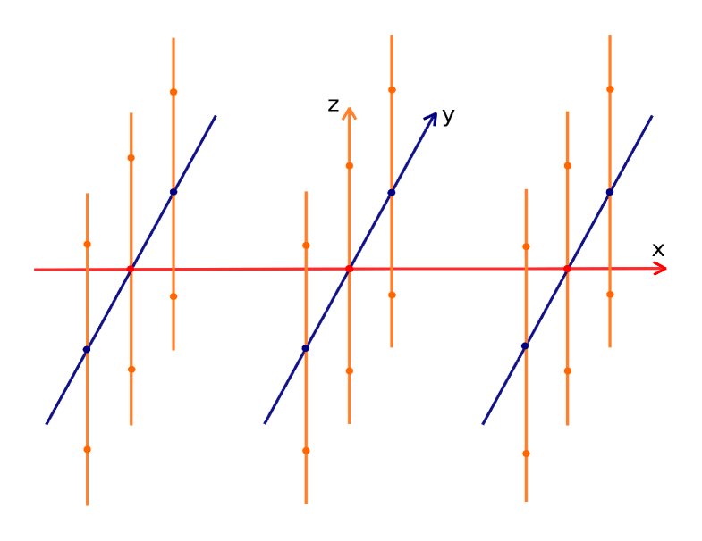
In this paper we investigate a diffusion process on a -comb (see Fig. 1) with stochastic resetting. The diffusion on a three dimensional comb is governed by the following equation
| (1) |
where
is the Fokker-Planck (transport) operator, and , and are the diffusion coefficients along the , and directions, respectively. The -functions in front of the second spatial derivative with respect to , mean that diffusion along the backbone (-axis) is allowed only at , while the -function in front of the second spatial derivative with respect to , means that the diffusion along the main fingers (or branches) (-axis) is allowed only at . The -axis is a secondary finger, an auxiliary direction along which the particle performs normal diffusion.
On the other hand, the diffusion process in one dimension under stochastic resetting was introduced by Evans and Majumdar maj1 . The corresponding equation is given by
| (2) |
where the initial position reads , is the diffusion coefficient, is the rate of resetting to the initial position, the second term on the right hand side represents the loss of probability from the position due to reset to the initial position , and the third term is the gain of probability at due to resetting from all other positions. This equation represents a renewal process: each resetting event to the initial position renews the process at a rate . Between two consecutive renewal events, the particle undergoes free diffusion maj1 . It is known that this equation has a stationary solution in the long time limit given by
Afterwards, other types of motion and resetting mechanisms have been studied by introducing the two resetting terms to the Fokker-Planck equation of the corresponding process maj2 ; EvMa14 ; maj3 ; DuHe14 ; Pa15 ; ChSc15 ; Ma19 ; Gu19 ; lenzi_front . For instance, space-dependent reset rates maj2 or diffusion in a potential landscape Pa15 and the telegraphers equation Ma19 have been analyzed under this perspective. Other works have studied motion with resetting by employing a renewal equation MoVi13 ; mendez ; pal1 ; NaGu16 ; EuMe16 ; MoMaVi17 ; Sh18 ; EvMa18 ; axel ; MaCaMe19p ; BoChSo19 ; BoChSo19p ; MaCaMe19pp ; MaCaMe19ppp , which has also been used to study the completion time of search processes with resetting CaMe15 ; reu ; pal reu ; chechkin ; pal pre ; pal prr ; masoliver2019 .
Multi-dimensional diffusion has already been studied in the literature EvMa14 . There, diffusion with resets in an multi-dimensional, homogeneous, infinite media is studied. In this work we analyze the transport properties and the long time behavior of diffusion in an heterogeneous environment and determine the properties emerging from resetting in the different space coordinates.
The paper is organized as follows. In Section II we consider diffusion in a three-dimensional comb with global exponential (Markovian) resetting. We give exact results for the marginal probability density functions (PDFs), stationary distributions and MSDs along all three axes. We also confirm the analytical results by numerical simulations by employing a Langevin equation approach for comb structure. Excellent agreement has been shown. Diffusion in three-dimensional comb with exponential resetting to the backbone is considered in Section III and the corresponding PDFs and MSDs are also found. In Section IV exponential resetting to the fingers is analyzed. We also discuss the resetting mechanisms in two-dimensional comb-structures in Section V. In Section VI we give detailed explanation of the topological constraint of the transport properties of both two- and three-dimensional comb structures. Summary is provided in Section VII.
II Global resetting
II.1 Analytical results
We start our analysis by considering diffusion in a three dimensional comb with global resetting, represented by the equation
| (3) |
with the initial position . This equation can also be interpreted in terms of a renewal process: each resetting event to the initial position renews the process at a rate . Between two consecutive renewal events, the particle undergoes diffusion on the -comb structure.
To find the solution of Eq. (II.1) we apply the Fourier transformations†††The Fourier transform of a function is given by . The inverse Fourier transform then reads . with respect to , and , and the Laplace transformation‡‡‡The Laplace transform of a function reads . with respect to . Therefore, for the PDF in the Fourier-Laplace domain we obtain, see Supplemental material 1 for details of calculations,
II.2 Marginal PDFs
In order to analyze the motion along all three directions, we analyze the marginal PDFs,
| (5) | |||
| (6) | |||
| (7) |
In the Fourier-Laplace space, the marginal PDFs are
| (8) |
| (9) |
| (10) |
Therefore, from Eqs. (II.1) and (8), for the marginal PDF along the backbone we have
| (11) |
where . By applying the inverse Fourier transform we obtain
| (12) |
From Eq. (11), by inverse Fourier-Laplace transforms we arrive at the generalized (non-Markovian) diffusion equation along the backbone
| (13) |
where
| (14) |
Here
| (15) |
is the three parameter Mittag-Leffler function prabhakar §§§The Laplace transform of the three parameter Mittag-Leffler function reads prabhakar Its asymptotic behaviors are given by garrappa ; pre2015 and is the Pochhammer symbol. The initial condition is . The equation can also be written in the form
| (16) |
where
| (17) |
is a so-called regularized Prabhakar derivative polito , which has many applications nowadays sandev mathematics ; epl ; weron . The stationary PDF along the backbone, obtained in the long time limit, becomes
| (18) |
From Eqs. (II.1) and (9), for the PDF along the fingers we find
| (19) |
where . From here, by applying the inverse Fourier transform we obtain
| (20) |
The marginal PDF provides the transport equation along the main finger and it is governed by the equation
| (21) |
with the initial condition . Here the kernel is
| (22) |
Eq. (21) can also be presented by means of the regularized Prabhakar derivative (17). It reads
| (23) |
or equivalently
| (24) |
where is the error function, while
| (25) |
is the tempered Caputo derivative with the exponential truncation, where is the truncation parameter fcaa2015 ; sandev mathematics . For the stationary PDF along the direction, we find
| (26) |
For the direction, we have
| (27) |
that yields
| (28) |
where . The corresponding equation for the transport along secondary fingers reads
| (29) |
where
| (30) |
and it can be rewritten in the equivalent form
| (31) |
which is a diffusion-absorption equation. The stationary PDF along the direction is
| (32) |
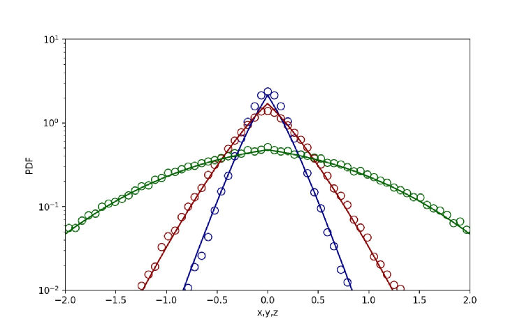
It is interesting to note that the obtained stationary PDFs along each axis are exponential functions, so that the global resetting does not modify the stationary state with respect to the case of standard diffusion in one dimension under resetting, see Eq. (2). The global resetting affects the transient dynamics towards the stationary state only. For a given value of for all three components, the width of the PDF varies. This can be seen from the analytical formulas, in which the width of the exponential stationary PDF depends on for the component, on for the component and on for the component, see Eqs. (18), (26), (32). The obtained analytical results are verified by stochastic simulations with the Langevin equation approach, see Section II.4.
II.3 Mean squared displacements
In the section, we analyze the MSDs along all three directions,
Taking into account corresponding solutions for the marginal PDFs, we have
| (33) |
where is the exponential integral function. This corresponds to the transition from subdiffusion to localization
For the fingers we have
| (34) |
that corresponds to the transition from subdiffusion to localization as well,
Eventually, the MSD for - fingers reads
| (35) |
that corresponds to saturation in the long time limit,
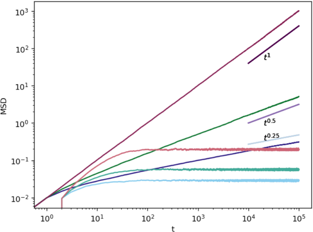
Therefore, unlike an initial transient behaviour all the MSDs saturate towards a constant value (exhibiting stochastic localization) as in the scenario of one-dimensional diffusion with resets. This confirms the existence of a non-equilibrium stationary state, which has been recently observed for many different dynamics under constant-rate resets axel . This variety of cases has been also obtained from stochastic simulations of the process based on a Langevin equation approach, see Section II.4.
II.4 Langevin equation approach. Numerical simulations
To verify the analytical solution obtained in the previous section, we perform numerical calculations, considering a system of Langevin equations iomin jstat ; lenzi njp , and where resets, as a renewal process, can be easily performed, see Ref. pal_pre2015 . The system of coupled Langevin equations reads
| (36d) | |||
| (36h) | |||
| (36l) | |||
where , , are constants related to the diffusion coefficients , , , , , are zero mean Gaussian noises (), and are functions introduced to mimic -functions (see Refs. iomin jstat ; jstat2020 ), and is the parameter of the Poisson process. To replicate the Dirac -function, diffusion across the and directions is permitted in a narrow band of thickness along the and axes. As a result, the noise in Eqs. (36d) and (36h) is multiplicative, however in Refs. lenzi njp ; jstat2020 the authors verified that the value has no influence in the diffusive process, as long as and the noise amplitudes , , are of the same order of magnitude. In our simulations, we have set . The noises , , , were sampled from a Gaussian distribution . The time evolution of the diffusive particle is a renewal process, where each resetting event to renews the process at a Poisson rate .
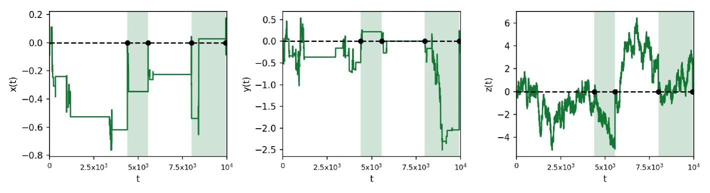
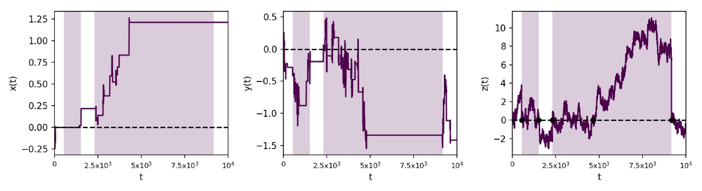
This effect of stochastic resetting is modeled by sampling a resetting time from an exponential distribution with parameter representing the time between two events in a Poisson point process. During this resetting time, the particle undergoes diffusion on the three-dimensional comb and resets at afterwards. Graphical representation of the simulations of particle trajectories along all directions is given in Fig. 2.
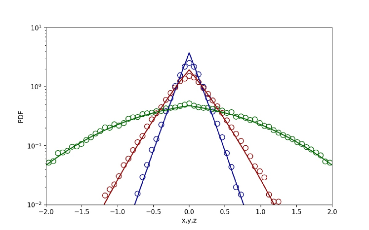
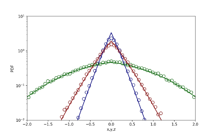
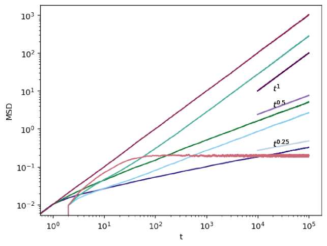
Regarding the simulation of marginal PDFs and temporal evolution of the variance, ensembles of particle positions were simulated considering a time step of across a time span of in order to observe convergence of the processes, with the MSD being calculated for each of the ensembles along all three directions , , . In Fig. 3 we give comparison of the analytical and simulation results for the marginal PDFs, where we use that , , with , see iomin jstat ; pal_pre2015 . In Fig. 4 we show the simulated time evolution of the MSDs in the three directions. From the simulation results one can verify that they are in a very good agreement with the saturation values obtained analytically, if one uses that . For more results on the corresponding PDFs obtained by the numerical simulations we refer to the Supplemental material 1.
III Resetting to the backbone
Global resetting takes the particle to a particular position of the comb (with the coordinates in Eq. (II.1)). However, it is only one of many possible mechanisms of resetting. Here, we proceed with a slightly softer resetting procedure, which takes the particle to the backbone. This resetting is applied to the and directions only, taking a walker being at to the point . In this case, the governing equation reads
which differs from Eq. (II.1) in the last term only. This difference results from the difference between the global resetting and resetting to the backbone. In the former case the particle is taken at the particular position as stated by the term in Eq. (II.1). However, in the latter case, considered here, the particle appears at but the position is not modified. Mathematically it can be written as the marginal distribution, the double integral term in Eq. (81). From the Fourier-Laplace transformations, we arrive at the following PDF in the Fourier-Laplace space, see Supplemental material 2 for details,
| (38) |
From this equation, the marginal PDFs for the three axis can be straightforwardly obtained as done in the previous section:
| (39) |
| (40) |
| (41) |
Here we note that the corresponding equations, Eqs. (40) and (41), for the marginal PDFs along the and directions are the same as in the case of global resetting, Eqs. (20) and (27), respectively. Along the backbone the PDF is
| (42) |
which is governed by the equation
| (43) |
where is the tempered fractional derivative (25) of order .
The corresponding MSDs along and axes are the same as those for the case of global resetting, since the effect of the resetting in these two dimensions is equivalent for both scenarios. However, the dynamics on the axis change substantially as reflected in the MSD
| (44) |
Its asymptotics reads
| (48) |
. The resetting mechanism studied in this section enhances the transport since it returns particles to the axis. Consequently, instead of the saturation of a stationary value for the MSD, one can see from Eq. (100) that in the long time limit, , i.e. it scales diffusively. The short time limit scales as , as in the case of global resetting. This means that we observe accelerating transport along the backbone, ranging from subdiffsuion to normal diffusion.
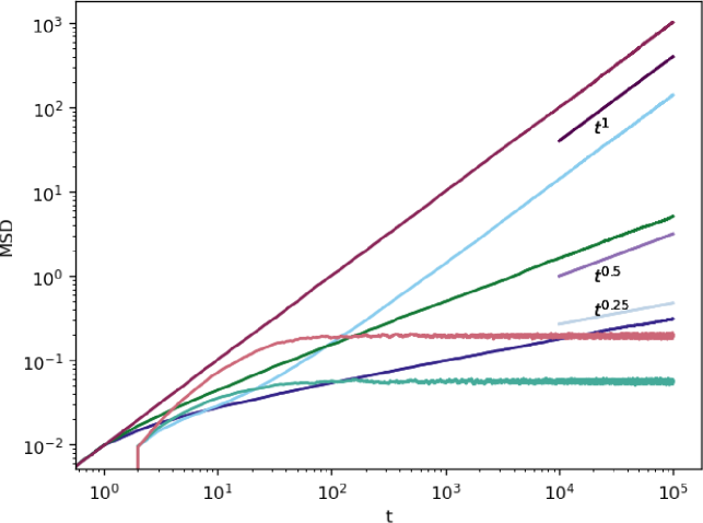
The numerical simulations of particle trajectories along all three directions, by using the Langevin equations approach, are shown in Fig. 5. We see that while in the and axis we observe recurrent returns to the origin, in the axis the motion does not return. Instead, it freely moves away from the origin. In Fig. 6 we give comparison of the analytical and simulation results for the marginal PDFs from where one observes excellent agreement between both approaches. Same parameters for , and as in the case of global resetting are used. The analytical results has also been confirmed by simulation results of the MSDs given in Fig. 7, where the and components of the MSD reach a stationary value while the MSD in the direction increases linearly. This is in agreement with the analytical results found above. More simulation results for the PDFs are given in the Supplemental material 2.

IV Resetting to the main fingers
Finally, we study the dynamics of the system when the resetting applies to particle located at any secondary finger along the axis and moves to main finger (axis in Fig. 1). In this case, the governing equation reads
| (49) |
where the last term is now the marginal distribution in the variables and . In the Fourier-Laplace space, the solution of the equation reads, see Supplemental material 3 for details,
| (50) |
This also yields the images of the marginal PDFs for the different axis. Eventually, we have
| (51) |
| (52) |
| (53) |
From these expressions one obtains the corresponding MSDs, which are
| (54) |
| (55) |
and the MSD along the axis is the same as in the previous cases. Their asymptotics read
| (59) |
| (63) |
In this case, the MSD in the -axis behaves subdiffusively with as in the case with no resetting, and then it turns to , which means an accelerating subdiffusive transport. Along the -axis, the MSD scales as in the short time limit, and then it turns to linear dependence in time . Along the -axis the MSD from the normal diffusive behavior reaches a stationary value in the long time limit.
We also performed numerical simulations by using the Langevin equations approach. Same parameters for , and as previous are used. The simulation results show very good agreement with the analytical results, see Figs. 8, 9 and 10. For more details on analytical computation and simulation results see also Supplemental material 3.
V Remarks on two dimensional comb
Here we note that the results obtained for the three-dimensional -comb can be used for the two-dimensional -comb. The and axes in the three-dimensional comb would correspond to the and axes in the two-dimensional comb. Therefore, the results obtained for the and directions in the three-dimensional comb with resetting in the backbone correspond to the results for the and directions in the two-dimensional comb with global resetting. Furthermore, the results obtained for the and directions in the three-dimensional comb with resetting in the main fingers correspond to the results for the and directions in the two-dimensional comb with resetting in the fingers.
VI Remark on the three dimensional comb geometry
The topological (comb) constraint of the transport properties of both two- and three-dimensional combs should be discussed as well. To that end, let us understand the role of the and functions in the highly inhomogeneous diffusion coefficients in Eq. (1). One should recognize that the singularity of the and components of the diffusion tensor is the intrinsic transport property of the comb model (1). Note that this singularity of the diffusion coefficients relates to a non-zero flux along the backbone and fingers, and for the two dimensional case it was discussed in Refs. dvork2009 ; LZ98 ; IoZaPf16 ; SaIoMe16 . Here, we extend the arguments of Refs. IoZaPf16 ; SaIoMe16 for the three dimensional case of Eq. (1). Let us consider the Liouville equation
| (64) |
where the three dimensional current describes Markov processes in Eq. (1). In this case, the three-dimensional current reads
| (65a) | |||
| (65b) | |||
| (65c) | |||
Here, we take a general diffusivity function in the and directions and , respectively (instead of and in Eq. (1)). Therefore, Eq. (64) together with Eqs. (65), can be regarded as the three-dimensional non-Markovian master equation.
Integrating Eq. (64) with respect to and from to : and , one obtains for the l.h.s. of the equation, after application of the middle point theorem, , which is exact in the limit . This term can be neglected in this limit . Considering integration of the r.h.s. of the equation, one should bear in mind that this procedure is artificial and its implementation needs some care. First we consider the currents outside of the vicinity of the backbone. In this case, according to the comb geometry, and we consider a two-dimensional comb. Therefore, we perform integration with respect to only. From Eq. (65c) we obtain that this term responsible for the transport in the direction reads
where prime means derivative with respect to . This corresponds to the two outgoing fluxes from the fingers in the directions: . The transport in the direction, after integration, is
It should be stressed that the second derivative over , presented in the form
ensures both incoming and outgoing fluxes for along the direction at a point . Following the Kirchhoff’s law, we have for every point and at . Function contains both incoming and outgoing fluxes of the probability, while and are both outgoing probability fluxes. If the latter outgoing fluxes are not zero, the flux has to be nonzero as well: , as containing an incoming flux. Therefore, . Taking , one obtains in the limit a nonzero flux with , which is the diffusion coefficient in the direction in Eq. (64).
Now we perform integration in the vicinity of the backbone, where we take into account the singularity of the component of diffusion coefficient, which is . We also admit that integration of the current in Eq. (65c) with respect to yields zero. Therefore, integration with respect to and yields from Eq. (65b) the term responsible for the transport in the direction as follows
Here prime means derivative with respect to . This corresponds to the two outgoing fluxes from the backbone in the directions: . The transport along the direction, after integration of Eq. (65a), is
In complete analogy with the coordinate, the second derivative with respect to , presented in the form
as , ensures both incoming and outgoing fluxes for along the direction at a point . Again, after the integration, the Liouville equation is a kind of the Kirchhoff’s law: for each point and at . Note, that the flax in the direction is zero due to the integration with respect to . Since outgoing fluxes are not zero, and correspondingly the flux has to be nonzero as well: . Therefore, . Now, taking the diffusion coefficient in the form , one obtains in the limit a nonzero flux with , which is the diffusion coefficient in the direction in Eqs. (1), (64) and (65a).
VII Summary
We have studied the dynamics of a particle, which diffusing in a three-dimensional heterogeneous comb-like structure performs different types of resets. The hierarchical structure of the three-dimensional comb allows to study different resetting mechanisms that generate a wide variety of dynamics depending on the strength of the resetting mechanism. In particular, we studied thee types of resets in the three-dimensional comb and their influence on the dynamics of the MSD, and we found that at the short time there is no influence on the transport exponents, which remain the same as in the case without resetting. However, at the long time limit, the system is strongly affected by the resetting process which leads a change in the transport exponents.
We studied three kinds of resetting: global resetting of a particle from any point on the comb to a fixed point at and two kinds of softer resetting, where two coordinates and one coordinate are fixed. When resets are global, the MSDs in , and directions reach constant values exhibiting stochastic localization, i.e. a non-equilibrium steady state is reached. This result is in complete agreement with the results observed for the dynamics of walkers with constant rate resetting recently studied in the literature maj1 ; axel . For a softer version of resetting consisting with two fixed coordinates, the walker returns to any positions at the backbone. It means that if the position of the walker before the resetting is , then after the reset it is . In this case, the dynamics for the and axis remains the same as in the global resetting case, since the effect of the resetting to these two coordinates is the same. However, in the direction, the resetting enhances the motion: it becomes subdiffusive for short times and then normal diffusion takes place for the long time scale. The latter regime results from the fact that the mean waiting time to stay in fingers becomes finite due to resetting. Indeed, the reset time PDF now plays the role of a waiting time PDF for the motion along the backbone ( direction). Since the reset time PDF is exponential (i.e., constant rate resetting or Markovian resetting process), the motion in the direction becomes diffusive in the long time limit. For the softer resetting with one fixed -coordinate, a stationary regime takes place in the fingers only. In the and directions the transport is enhanced with the MSDs behaving as follows: and . The obtained diffusion equations for the marginal PDFs shed light on the physical relevance of usage of the regularized Prabhakar derivative in diffusion theory. They could describe diffusion processes on comb structures with stochastic resetting.
Acknowledgment
This research was partially supported by Grant No. CGL2016-78156- C2-2-R (VM and AM). TS was supported by the Alexander von Humboldt Foundation.
References
- (1) A. Iomin, V. Méndez and W. Horsthemke, Fractional Dynamics in Comb-like Structures (World Scientific, 2018).
- (2) V. Méndez and A. Iomin, Chaos, Solitons & Fractals 53, 46 (2013).
- (3) A. Iomin and V. Méndez, Chaos, Solitons & Fractals 82, 142 (2016).
- (4) M. R. Evans and S. N. Majumdar, Phys. Rev. Lett. 106, 160601 (2011).
- (5) M. R. Evans and S. N. Majumdar, J. Phys. A: Math. Theor. 44, 435001 (2011).
- (6) M. R. Evans and S. N. Majumdar, J. Phys. A: Math. Theor. 47, 285001 (2014).
- (7) S. Gupta, S. N. Majumdar, and G. Schehr, Phys. Rev. Lett. 112, 220601 (2014).
- (8) X. Durang, M. Henkel, and H. Parl, J. Phys. A: Math. Theor. 47, 045002 (2014).
- (9) A. Pal, Phys. Rev. E 91, 012113 (2015).
- (10) C. Christou and A. Schadschneider, J. Phys. A: Math. Theor. 48, 285003 (2015).
- (11) J. Masoliver, Phys. Rev. E 99, 012121 (2019).
- (12) D. Gupta, J. Phys. A: Math. Theor. 47, 033212 (2019).
- (13) A. A. Tateishi, H. V. Ribeiro, and E. K. Lenzi, Front. Phys. 5, 52 (2017).
- (14) M. Montero and J. Villarroel, Phys. Rev. E 87, 012116 (2013).
- (15) V. Méndez and D. Campos, Phys. Rev. E 93, 022106 (2016).
- (16) A. Pal, A. Kundu, and M. R. Evans, J. Phys. A: Math. Theor. 49, 225001 (2016).
- (17) A. Nagar and S. Gupta, Phys. Rev. E 93, 060102 (2016).
- (18) S. Eule and J. J. Metzger, New J. Phys. 18, 033006 (2016).
- (19) M. Montero, A. Masó-Puigdellosas and J. Villarroel, Euro. Phys. J. B 90, 176 (2017).
- (20) V. P. Shkilev, Phys. Rev. E 96, 012126 (2017).
- (21) M. R. Evans and S. N. Majumdar, J. Phys. A: Math. Theor. 52, 01LT01 (2018).
- (22) A. Masó-Puigdellosas, D. Campos, and V. Méndez, Phys. Rev. E 99, 012141 (2019).
- (23) A. Masó-Puigdellosas, D. Campos, and V. Méndez, J. Stat. Mech.: Theor. Exp. 2019, 033201.
- (24) A. S. Bodrova, A. V. Chechkin, and I. M. Sokolov, Phys. Rev. E 100, 012119 (2019).
- (25) A. S. Bodrova, A. V. Chechkin, and I. M. Sokolov, Phys. Rev. E 100, 012120 (2019).
- (26) A. Masó-Puigdellosas, D. Campos, and V. Méndez, Front. Phys. 2019 00112.
- (27) A. Masó-Puigdellosas, D. Campos, and V. Méndez, Phys. Rev. E 100, 042104 (2019).
- (28) D. Campos, and V. Méndez, Phys. Rev. E 92, 062115 (2015).
- (29) S. Reuveni, Phys. Rev. Lett. 116 170601 (2016).
- (30) A. Pal and S. Reuveni, Phys. Rev. Lett. 118, 030603 (2017).
- (31) A. Chechkin and I. M. Sokolov, Phys. Rev. Lett. 121, 050601 (2018).
- (32) U. Basu, A. Kundu, and A. Pal, Phys. Rev. E 100, 032136 (2019); A. Pal and V. V. Prasad, Phys. Rev. E 99, 032123 (2019).
- (33) J. Masoliver and M. Montero, Phys. Rev. E 100, 042103 (2019).
- (34) A. Pal and V. V. Prasad, Phys. Rev. Research 1, 032001 (2019).
- (35) I. S. Gradshteyn and I. M. Ryzhik, Table of Integrals, Series, and Products (Academic Press, San Diego, 2007).
- (36) A. M. Mathai, R. K. Saxena and H. J. Haubold, The -function: Theory and Applications ( Springer, 2010).
- (37) T. Sandev, A. Chechkin, H. Kantz, R. Metzler, Fract. Calc. Appl. Anal. 18, 1006 (2015).
- (38) R. Garra and R. Garrappa, Commun. Nonlinear Sci. Numer. Simul. 56, 314 (2018).
- (39) T. Sandev, A. V. Chechkin, N. Korabel, H. Kantz, I. M. Sokolov, and R. Metzler, Phys. Rev. E 92, 042117 (2015).
- (40) T. R. Prabhakar, Yokohama Math. J. 19, 7 (1971).
- (41) M. D’Ovidio and F. Polito, Theory Probab. Appl. 62, 552 (2018); arXiv:1307.1696 (2013); R. Garra, R. Gorenflo, F. Polito, and Z. Tomovski, Appl. Math. Comput. 242 576 (2014).
- (42) T. Sandev, Mathematics 5, 66 (2017); T. Sandev, W. Deng, and P. Xu, J. Phys. A: Math. Theor. 51, 405002 (2018).
- (43) T. Sandev and A. Iomin, Europhys. Lett. 124, 20005 (2018).
- (44) A. Stanislavsky and A. Weron, Phys. Rev. Research 1, 023006 (2019); A Stanislavsky, A Weron, J. Chem. Phys. 149, 044107 (2018).
- (45) V. Méndez, A. Iomin, W. Horsthemke and D. Campos, J. Stat. Mech. 2017, 063205 (2017).
- (46) H. V. Ribeiro, A. A. Tateishi, L. G. A. Alves, R. S. Zola and E. K. Lenzi, New J. Phys. 16, 093050 (2014).
- (47) A. Pal, Phys. Rev. E 91, 012113 (2015).
- (48) E. K. Lenzi, T. Sandev, H. V. Ribeiro, P. Jovanovski, A. Iomin, and L. Kocarev, J. Stat. Mech. doi: 10.1088/1742-5468/ab7af4 (2020).
- (49) O.A. Dvoretskaya, P.S. Kondratenko, and L.V. Matveev, JETP 110, 58 (2010).
- (50) I.A. Lubashevskii and A.A. Zemlyanov, JETP 87, 700 (1998).
- (51) A. Iomin, V. Zaburdaev and T. Pfohl, Chaos, Solitons & Fractals 92, 115 (2016).
- (52) T. Sandev, A. Iomin, and V. Méndez, J. Phys. A: Math. Theor. 49, 355001 (2016).
Supplemental material: Stochastic resetting on comb-like structures, V. Domazetoski, A. Masó-Puigdellosas, T. Sandev, V. Méndez, A. Iomin and L. Kocarev
.1 Solutions for diffusion with global resetting
The diffusion equation in a three-dimensional comb with global resetting can be represented by
| (66) |
Here we consider the initial condition . The Laplace transformation of Eq. (.1) reads
| (67) |
Then, by Fourier transform with respect to , and we obtain
| (68) |
from where it follows
| (69) |
The inverse Fourier transform with respect to yields
| (70) |
from where we find ,
| (71) |
By applying the inverse Fourier transform with respect to , we have
| (72) |
and thus
| (73) |
Therefore, we finally obtain
| (74) |
After we find the marginal PDFs we will analyze the mean squared displacements along all three directions, , , and . Therefore, we have
| (75) |
where
| (76) |
is the three parameter Mittag-Leffler function, and is the Pochhammer symbol, is the exponential integral function,
| (77) |
where gives the error function, and
| (78) |
The Laplace transform of the three parameter Mittag-Leffler function (76) reads
| (79) |
and its asymptotic behaviors are given by
| (80) |
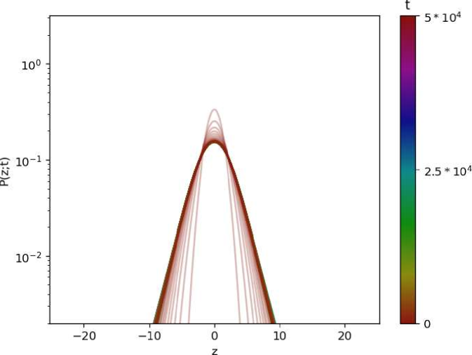
In Figs. 11, and 12, we give graphical representations of the PDFs of the process without resetting and under global resetting. The results are obtained by numerical simulations similar to the ones elaborated in Sec. II.4, with different values of the ensemble size of and the time span of .
(a) 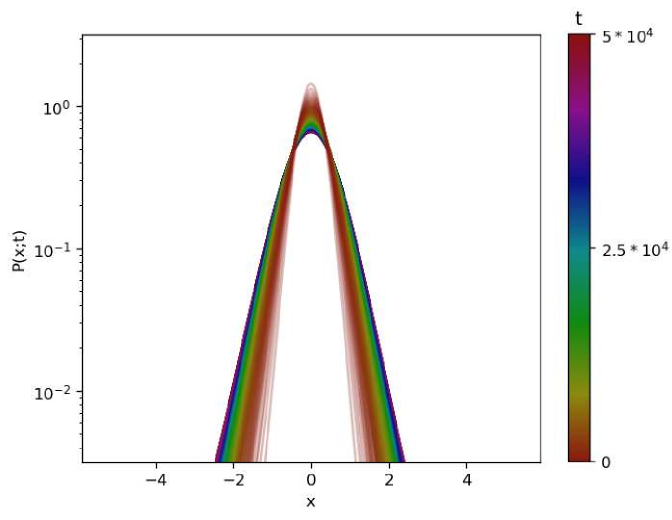 (b)
(b) 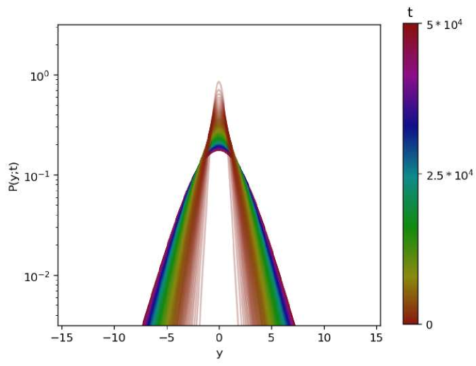
(c) 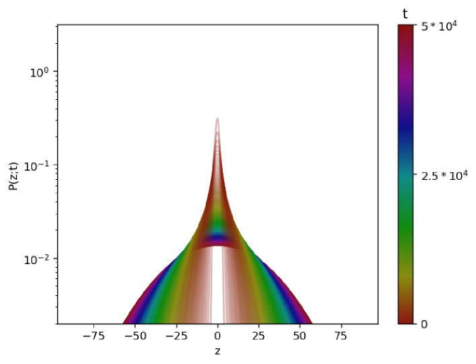
(a) 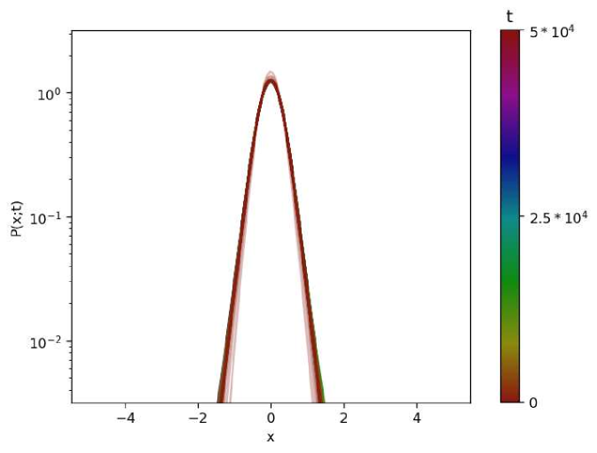 (b)
(b) 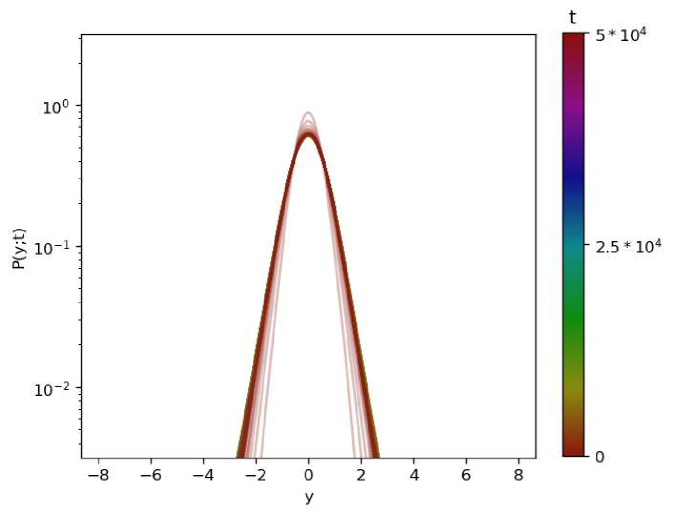
(c) 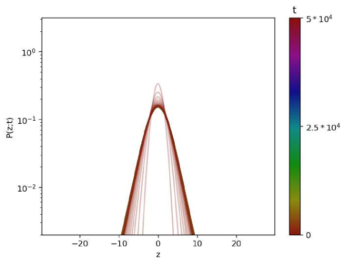
.2 Solutions for diffusion with reseting to the backbone
Previously we have studied a resetting mechanism which takes the particle to a particular position of the comb, the coordinate . Here, we proceed to analyse a slightly different resetting procedure, consisting on taking the particle to the backbone. This is, if the particle is at any position , the resetting consists on taking it to the position of the state space. In this case, the Fokker-Planck equation reads
| (81) |
Here, instead of appearing at the particular position as stated by , the particle appears at but the position is not modified and, therefore, it can be mathematically written as the marginal distribution (double integral term in Eq. (81)). In order to solve the equation for the propagator , we apply the Fourier-Laplace transform as done in the previous case to obtain
| (82) |
Now, isolating the propagator one gets
| (83) |
Let us proceed to find the three unknown terms on the right hand side. Taking one can isolate
| (84) |
with which the equation for the propagator reads
| (85) |
The other two terms can be obtained by taking the inverse Fourier transform of and and evaluating at and respectively. Starting by the last, one gets that
| (86) |
Proceeding similarly for the variable one gets
| (87) |
Putting all the elements into Eq. (85) and simplifying some terms one gets the following explicit expression for the propagator:
| (88) |
Finally, from these expressions one can get the corresponding MSD,
| (89) |
| (90) |
| (91) |
In Fig. 13, we give graphical representations of the PDFs of the process under resetting to the backbone.
(a) 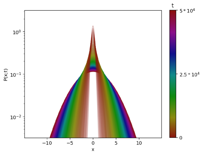 (b)
(b) 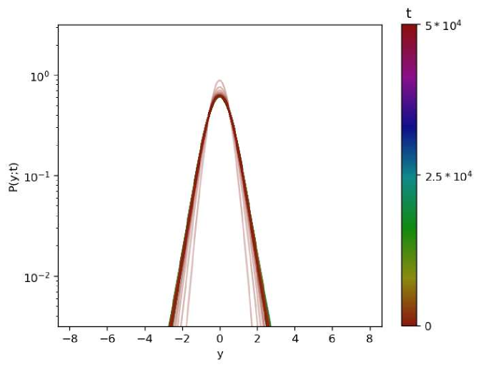
(c) 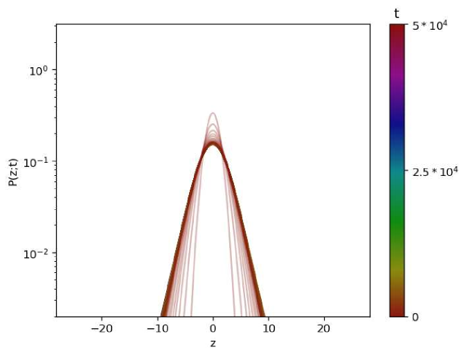
.3 Solutions for diffusion with reseting to the main fingers
Finally, we study the dynamics of the system when, instead of taking the particle to a fixed position in the axis or to the backbone, the resetting only applies to the axis, taking the particle to the corresponding main finger. In this case, the governing equation reads
| (92) |
where the last term is now the marginal distribution in the variables and instead of only the variable. The corresponding equation in the Fourier-Laplace space reads
| (93) |
from which the propagator can be isolated to give
| (94) |
and, by taking , we can isolate the following expression for the marginal PDF:
| (95) |
Introducing this expression to Eq. (94) we get
| (96) |
As done for the previous cases, the two unknown terms remaining on the right hand side can be found by applying the inverse Fourier transform with respect to the and variables to Eq. (96) and evaluating at . Starting by the last, one finds that
| (97) |
and proceeding equally for the variable:
| (98) |
Putting all the elements together one finds a formal expression for the propagator:
| (99) |
Finally, the corresponding MSD in the Laplace space read
| (100) |
| (101) |
| (102) |
In Fig. 14, we give graphical representations of the PDFs of the process under resetting to the backbone.
(a) 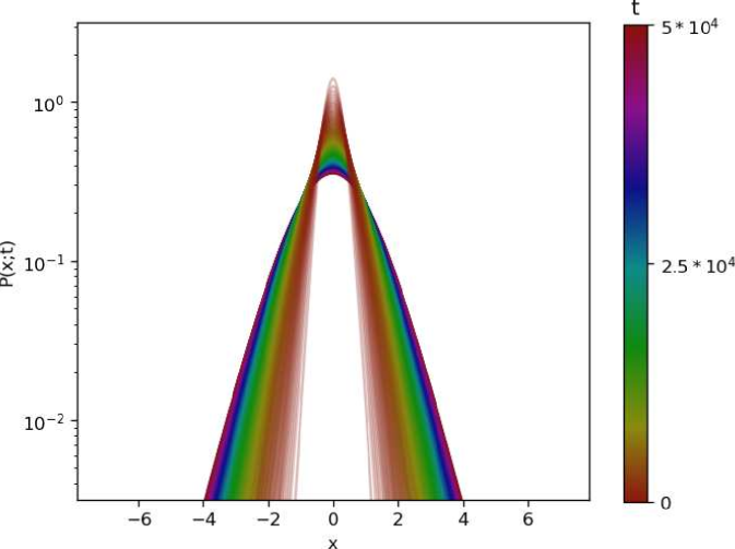 (b)
(b) 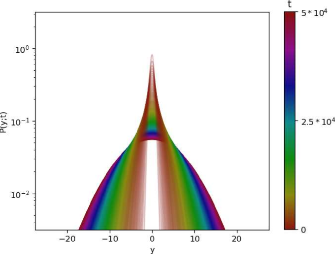
(c)