Stochastic thermodynamics of Brownian motion in a flowing fluid
Abstract
We study stochastic thermodynamics of over-damped Brownian motion in a flowing fluid. Unlike some previous works, we treat the effects of the flow field as a non-conservational driving force acting on the Brownian particle. This allows us to apply the theoretical formalism developed in a recent work for general non-conservative Langevin dynamics. We define heat and work both at the trajectory level and at the ensemble level, and prove the second law of thermodynamics explicitly. The entropy production (EP) is decomposed into a housekeeping part and an excess part, both of which are non-negative at the ensemble level. Fluctuation theorems are derived for the housekeeping work, the excess work, and the total work, which are further verified using numerical simulations. A comparison between our theory and an earlier theory by Speck et. al. is also carried out.
I Introduction
The theory of Brownian motion [1, 2] is not Galilean invariant, even though the underlying microscopic Newtonian dynamics does have this symmetry. The reason for the lack of Galilean symmetry is obvious: the ambient fluid is macroscopically at rest only in one particular inertial frame. It is only in this frame that the effects of fluid can be modeled as friction and random force as in the classical theory of Brownian dynamics. If the fluid is in global motion with a uniform velocity , one can transform to the co-moving frame (where the fluid is at rest) and apply the usual theory of Brownian motion. Translating back into the lab frame, the friction force becomes , which is proportional to the velocity relative to the fluid, whereas the random force remains the same. Now consider a fluid that is shearing or compressing, with a position (and possibly time) dependent velocity . The above chain of argument is not as compelling, since the co-moving frame is constantly deforming and therefore is not an inertial frame. Nonetheless, as long as the flow field is small, it is reasonable to assume that the friction force is approximately .
Stochastic thermodynamics [3, 4, 5, 6, 7, 8, 9] fuses stochastic dynamics with thermodynamics to form a unified framework for non-equilibrium statistical mechanics. In the standard theory of stochastic dynamics, the environment is usually assumed to be an equilibrium fluid at rest. In a pioneering work [10], Speck et. al. applied the above idea of Galilean transform to study stochastic thermodynamics of over-damped Brownian motion in a moving fluid. In the co-moving frame, the heat is defined as the work done by the friction and the random force, as in the standard theory of stochastic thermodynamics. Further defining the external potential as the fluctuating internal energy of the Brownian particle, they sketched a framework of stochastic thermodynamics for over-damped Brownian motion in moving fluid. This work was followed by several later works [11, 12, 13, 14, 15, 16], which carried out more detailed analyses and simulations of fluctuation theorems in shearing fluid. Three peculiar features are coming out of this theory. (For details, see Sec. IV of the present work.) Firstly it leads to fluctuation theorems for the integrated work only if the non-equilibrium processes start from equilibrium states where the flow field is completely turned off. The theory is therefore inapplicable to processes happening in steady flow. Secondly, the entropy production (EP) is positive only for incompressible flow. Finally, the EP in this theory cannot be decomposed into two positive parts. Hence no separate fluctuation theorem can be established for the housekeeping part and the excess part of the total EP. This is at odds with the basic structure of stochastic thermodynamics for systems lacking instantaneous detailed balance, as established by Jarzynski and Esposito, van den Brock et. al. [17, 18, 19, 20, 21].
It is well known that heat in stochastic thermodynamics is related to the time reversal of non-equilibrium processes through the condition of local detailed balance. It turns out that in the theory of Ref. [10], time reversal means reversal of both the time axis and the flow field. Since the environment, i.e. the shearing fluid has a well-defined temperature, the heat is further related to the environmental entropy change via . It is important to note, however, that the entropy change calculated this way is a microscopic quantity, whereas the true entropy change of the environment is extensive in the size of the shear fluid. Hence the EP calculated in the theory of Ref. [10] can only be a tiny part of the physical EP in the joint system of Brownian particle and shearing fluid. This subtlety is shared by all models of stochastic thermodynamics embedded in dissipative backgrounds, such as Brownian motion in temperature gradients [22]. With this subtlety carefully remembered, the fluctuation theorems, when formulated in terms of integrated work, are nonetheless valuable tools for understanding of the statistical properties of non-equilibrium processes.
In this work, we shall try an alternative approach to the problem. Instead of transforming to the co-moving, we shall stay in the lab frame and treat the effects of the flow field as a non-conservative force acting on the Brownian particle. This allows us to apply the general framework of stochastic thermodynamics developed in Ref. [21] for non-conservative Langevin systems. In our theory, the time reversal of process means the reversal of only the time-axis, but not of the flow field. Consequently, the heat defined in our theory is inequivalent to that defined in Ref. [10]. As discussed in great detail in Ref. [21], in the absence of instantaneous detailed balance, there are also ambiguities in the definition of system energy. Different definitions of energy lead to different (but equivalent) formulations of stochastic thermodynamics. The situation is not unlike the gauge redundancy in electromagnetism. We shall adopt the so-called Gibbs gauge where the instantaneous non-equilibrium steady state (NESS) has the form of Gibbs-Boltzmann distribution, which leads to great simplification of the theoretical formalism.
The key results of the present work can be summarized as follows: (i) The EP at the ensemble level that emerges from our theory is positive definite for arbitrary flow field. (ii) The EP can be decomposed into a housekeeping part and an excess part, both of which are positive. (iii) At the trajectory level, both the housekeeping work and the excess work obey a fluctuation theorem. (iv) These fluctuation theorems are applicable for arbitrary processes starting from arbitrary non-equilibrium NESSs, including equilibrium states as special cases. Overall, therefore, the present theory has a wider range of applicability than that of Ref. [10].
The remaining of this work is organized as follows. In Sec. II we formulate the Langevin equation for Brownian motion in a following fluid. In particular, in Sec. II.2 we discuss the adjoint Brownian dynamics, in Sec. II.3 we perturbatively calculate the Gibbs gauge representation. In Sec. III we develop the theory of stochastic thermodynamics and derive fluctuation theorems for the housekeeping EP, the excess EP, and the total EP. In Sec. IV, we discuss the differences between our theory and the theory of Ref. [10]. In Sec. V we present numerical verifications of all fluctuation theorems. Finally in Sec. VI we draw concluding remarks and project future research directions.
II Brownian dynamics in a flow
II.1 Langevin equation
For simplicity, we examine two-dimensional Brownian dynamics in a fluid with time-independent flow. Generalization to three-dimensional time-dependent flow is straightforward. The velocity field of the fluid is
| (1) |
where are respectively the unit vectors along and directions, and . Assuming that the Brownian particle is further confined by an external potential , its motion can be described by the following over-damped Ito-Langevin equations:
| (2) |
where is the friction constant, is the temperature, and are the standard Wiener noises, which have the following basic properties:
| (3a) | |||||
| (3b) | |||||
Note that the first term in each of Eqs. (2) is the friction force multiplied by .
Equations (2) can be rewritten into:
| (4) |
where are given respectively by
| (5a) | |||||
| (5b) | |||||
where is an irrelevant normalization constant. We do not need to distinguish superscripts from subscripts because we will only use Cartesian coordinate systems. Equation (4) is a special case of the following covariant nonlinear Ito-Langevin equation with non-conservative forces [21] (with all repeated indices summed over):
| (6) |
where all variables are even under time reversal, and the matrices and are given respectively by
| (7) | |||||
| (8) |
Since both and are constants, in Eq. (6) vanishes identically. We shall call and respectively the generalized potential and the non-conservative force 111Strictly speaking, the non-conservative force is defined as in Ref. [21]..
The Langevin equation (4) is equivalent to the following covariant Fokker-Planck equation (FPE):
| (9) |
which can also be written in the form of:
| (10) |
where is the probability current:
| (11) |
It is easy to see that the following transformation:
| (12a) | |||||
| (12b) | |||||
leaves the combination invariant, and hence also leaves the Langevin equation (6) and the Fokker-Planck equation (9) as well as the probability current (11) invariant. Inspecting Eqs. (5a) and (5b), we see that the transform (12) may be understood as a simultaneous change of the external potential and the flow field that preserves the Brownian motion. We shall call it a gauge transformation. A particular decomposition of the combination into and shall then be called a gauge.
The most convenient gauge is the Gibbs gauge [21], where is related to the NESS via
| (13) |
Substituting this back into Eq. (11), we find the NESS probability current is then given by
| (14) |
which is proportional to . The fact that is non-vanishing characterizes the non-equilibrium nature of the NESS. Substituting Eq. (14) into the steady state FPE , we obtain the Gibbs gauge condition:
| (15) |
which, using Eq. (12), can be further rewritten into:
| (16) |
In Sec. II.3, we solve this nonlinear differential equation for the case of simple shear flow and harmonic confining potential, and use Eqs. (12) to determine for the Gibbs gauge.
II.2 Adjoint Langevin dynamics
We now define the adjoint Langevin dynamics, which is related to the original dynamics (17) via the following transform in the Gibbs gauge:
| (18) |
Using Eqs. (13) and (14), we see that the adjoint process has the same NESS pdf and opposite NESS probability current as the original process:
| (19) | |||||
| (20) |
Just as the original dynamics, the adjoint dynamics can also be realized by many different combinations of flow field and confining potential, each characterized by a pair that is related to via a gauge transformation:
| (21a) | |||||
| (21b) | |||||
which is the counterpart of Eqs. (12). The gauge function is arbitrary. The most convenient choice is:
| (22) |
Substituting this back into Eqs. (21), we may express in terms of . Combining these results with Eqs. (18), we obtain:
| (23a) | |||||
| (23b) | |||||
Substituting these into Eqs. (5), we find the confining potential and the flow field for the adjoint process:
| (24a) | |||||
| (24b) | |||||
Hence the flow field of the adjoint dynamics is the opposite of that of the original process.
II.3 Harmonic potential and simple shear flow
For numerical simulations (to be detailed in Sec. V), we shall only consider a harmonic confining potential and a simple shear flow:
| (25a) | |||||
| (25b) | |||||
Using Eqs. (5) we find
| (26a) | |||||
| (26b) | |||||
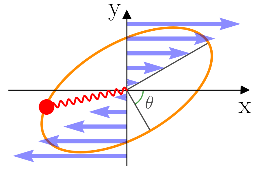
Note that has the dimension of inverse time, and is even under time reversal. The dimension of is inverse of length, and hence also even under time reversal. The shear flow and the confining potential are illustrated in Fig. 1, together with a contour line of the NESS pdf.
We define a dimensionless parameter , which characterizes the relative importance of the flow field compared with the confining potential. For colloidal particles in shearing fluid under typical experimental conditions, this parameter is expected to be much less than the unity, hence we expect that the flow field only leads to a small perturbation of the equilibrium distribution of the Brownian particle. Therefore we may solve Eq. (16) by expanding in terms of , and subsequently use Eqs. (12) to find and . Since the calculation is rather straightforward, we skip all details and directly present the second order results:
| (27a) | |||||
| (27b) | |||||
| (27c) | |||||
where the constant is such that Eq. (13) is normalized. We shall not need the concrete expression for . The reader may verify directly that Eqs. (27a) does satisfy the Gibbs gauge condition (15) up to .
If is not small, Eqs. (27) are not good approximations. Nonetheless, it is easy to see from Eq. (16) that, due to the quadratic nature of and the linear nature of , is quadratic in . Consequently, is also quadratic in , and is linear in . Contour lines of are therefore all ellipses, one of them being illustrated in Fig. 1. We can therefore set
| (28) |
and numerically find all coefficients . is determined by the condition of normalization. The numerical method is explained in App. A.1.
III Stochastic thermodynamics
In Ref. [21], we developed a unified theory of stochastic thermodynamics for Langevin systems driven by non-conservative forces and coupled to a single heat bath with temperature . The Langevin dynamics Eq. (6) is a special case of this unified theory, with all variables and control parameters being even under time reversal, and the kinetic matrix being symmetric and constant. We shall therefore follow the procedure developed in Ref. [21] (especially Sec. VI, which treats symmetric models) to develop the theory of stochastic thermodynamics.
It is important to emphasize that by formulating the Langevin equation into Eq. (17), we are taking the viewpoint that the effects of the flow field is treated as a non-conservative force field. The dissipation caused by the shearing fluid, which is extensive in the size of the fluid, is not a concern to us, since we are only interested in the dynamics of the Brownian particle.
In this work, we shall assume that the flow field is fixed and consider non-equilibrium processes where the force constant and the equilibrium position of the confining potential (25a) are systematically varied. For simplicity, we introduce the notations , and . It then follows that as well as all depend parametrically on . We will therefore use the notations etc.. In principle, the theory we develop is also applicable to processes where the flow field is also systematically varied. Experimentally, however, it is much more difficult to vary the flow field in a precisely controlled way.
III.1 Work, heat and EP
We define the fluctuating internal energy as
| (29) |
where is the generalized potential in Gibbs gauge, to be found by solving Eq. (15). The NESS distribution Eq. (13) can then be rewritten as
| (30) |
To realize such a NESS, one only needs to hold the shear flow and the control parameter fixed for a sufficiently long period of time. The equilibrium free energy is defined as
| (31) |
where in the second step we used the fact that is properly normalized. Hence our definition (29) of energy guarantees that the equilibrium free energy vanishes identically. This leads to certain simplification of the fluctuation theorems, as we shall see below.
We define differential heat at the trajectory level as
| (32) | |||||
where means differential of due to variation of , and is the stochastic product in Stratonovich’s sense:
| (33) |
The differential work at the trajectory level is defined as
| (34) | |||||
where is the differential of due to variation of .
The above defined heat and work can be decomposed into a housekeeping part and an excess part:
| (35) | |||||
| (36) |
where are respectively housekeeping heat and housekeeping work, whereas are respectively excess heat and excess work, defined as
| (37a) | |||||
| (37b) | |||||
| (37c) | |||||
| (37d) | |||||
The first law of thermodynamics at the trajectory level is given by either of the following two forms:
| (38) |
Note that the housekeeping heat and housekeeping work exactly cancel each other.
Heat and work at the ensemble level can be obtained by averaging the corresponding quantities at the trajectory level over both noises and the pdf of . To obtain a well-defined continuum limit, these differential quantities at the ensemble level must be computed up to the first order in . It is important to remember that the Wiener noises are square root of , and hence according to Eq. (17a), contains parts scaling with . Consequently, we need to expand these differential quantities up to the second order of , to keep all terms linear in .
As an example, let us compute the excess heat at the ensemble level:
| (39) |
where means double average over Wiener noises and over probability distribution of . First we use Eq. (37b) to expand up to the second order in :
| (40) |
where all products are in Ito’s sense. We now use the Langevin equation (17a) to express in terms of and . All terms in the form of and can be neglected, since they are higher order than . Then we average over the Wiener noises . Finally we multiply the result by the pdf and integrate over , and obtain the differential excess heat at the ensemble level:
| (41) |
where means average over the pdf of :
| (42) |
Similarly, the differential housekeeping heat at the ensemble level is given by
| (43) |
Further using the Gibbs gauge condition (15) we may rewrite the above result as
| (44) |
which is non-positive definite.
The differential housekeeping and excess work at the trajectory level can be similarly computed:
| (45) | |||||
| (46) |
The total heat and work at the ensemble level are then the sum of the corresponding housekeeping parts and excess parts:
| (47) | |||||
| (48) |
The system entropy is:
| (49) |
whose differential can be calculated using the Fokker-Planck equation:
| (50) | |||||
where in the last step we have integrated by parts.
The EP is defined as
| (51) |
where is defined as the environmental entropy change. As explained previously, is only the part of environmental entropy change that can be captured by our theory of stochastic thermodynamics. This can be further decomposed into a housekeeping EP and an excess EP :
| (52) | |||||
| (53) | |||||
| (54) |
In particular, in the NESS, the excess EP vanishes identically, whereas the housekeeping EP reduces to
| (55) |
where is the NESS current given in Eq. (14).
Further using Eqs. (50) and (41), as well as the Gibbs gauge condition (15), we may rewrite the excess EP in the following apparently positive form:
| (56) |
Hence EP is the sum of a positive housekeeping part and a positive excess part, a general feature of Markov systems with even variables and parameters that lack instantaneous detailed balance [17, 18, 19, 20].
Finally we may also define non-equilibrium free energy:
| (57) |
It is then easy to verify the following differential forms:
| (58) |
which may be further rewritten as
| (59) |
III.2 Transition probability
To study fluctuation theorems, it is necessary to know the short-time transition probability of the Langevin process defined by Eq. (17a). Let be respectively the initial position and the final position of an infinitesimal transition taking place during , and let be the mid-point. A general expression for the short-time transition probability of the Langevin equation (6) was derived in Eqs. (A4) of Ref. [21], using the general result of time-slicing path integral in Ref. [23]. Specializing to the Langevin dynamics Eq. (17a), we find 222The notation may be unfortunately confusing since we need to integrate over to verify the normalization of this transition probability density function. To avoid this confusion, we may replace by and remember that they are infinitesimal quantities. (Note that the notations are slightly different here)
| (60a) | |||||
| where the action is given by | |||||
| (60b) | |||||
where the subscript in Eq. (60b) means that all functions inside the bracket are evaluated at . The action is expanded up to the first order in , which is sufficient to guarantees a correct continuum limit. In fact it is ok to evaluate the second term in the r.h.s. of Eq. (60b) at any point, the resulting error is of higher order than , and hence is negligible in the continuum limit. Note that we show explicitly the dependence of the action on the non-conservative force .
Let us supply a heuristic explanation for Eqs. (60). First we note that the Wiener noises are infinitesimal Gaussian with basic properties (3). Using these we can readily construct their pdf:
| (61) |
Now given , the Langevin equation (17a) may be understood as a linear relation between and the infinitesimal displacement . Hence we may obtain the pdf for directly from Eq. (61):
| (62) |
Note that the action appearing in the exponent above is formally identical to the first term in the action (60b). It is important to note however as a basic property of Ito-Langevin equation, the function in (17a), which also appears in Eq. (62) is evaluated at the initial point . This should be contrasted with Eqs. (60), where the same function is evaluated at the mid-point . Because of the appearing in the denominator of the actions, however, this difference is qualitatively important and is compensated by the second term in the action (60b).
Using Eq. (60a), we can also compute the backward transition probability from to . All we need is to swap and in Eq. (60a). Note that and appear in Eq. (60a) only in the combinations and , which are respectively odd and even under the swap. Hence to obtain we only need to flip the sign of . This leads to
| (63a) | |||||
| (63b) | |||||
Recall the adjoint process defined in Sec. II.2 is related to the original process by changing the sign of . We can construct the corresponding transition probability for the adjoint process from Eqs. (60):
| (64a) | |||||
| (64b) | |||||
The backward transition probability of the adjoint process can be similarly obtained from Eqs. (63):
| (65a) | |||||
| (65b) | |||||
III.3 Four processes
| Process: |
|
|
Confining potential | Velocity field | ||||
| Forward | ||||||||
| Backward | ||||||||
| Adjoint Forward | ||||||||
| Adjoint Backward |
We keep the flow field fixed, and vary parameters systematically, which fully determines the Langevin dynamics. We call the dynamic protocol in the Gibbs gauge, and the dynamic protocol in the natural gauge. A dynamic process is determined by the initial pdf of together with the dynamic protocol either in the Gibbs gauge or in the natural gauge. Transformation between two dynamic protocols are given by Eqs. (12) and (5).
We define four processes as below, all of which start from and end at :
- 1.
-
2.
Backward process: The dynamic protocol is
(68a) (68b) The initial pdf is .
-
3.
Adjoint process: The dynamic protocol is
(69a) (69b) The initial pdf is .
-
4.
Adjoint backward process: The protocol is
(70a) (70b) The initial pdf is .
Note that each of these processes starts from the NESS corresponding to the initial control parameter of the dynamic protocol. Such an initial state can be realized easily in experiments. Note also that in general, the system is not in a NESS at the end of any of these processes.
The protocols of all these processes are displayed in the second and third columns of Table 1. We may also express these protocols in the natural gauge, in terms of the confining potential and the flow field. The results are displayed in fourth and fifth columns of Table 1.
A pivotal property of these processes is that the backward process, the adjoint process, and the adjoint backward process are all uniquely determined by the forward process. Furthermore, the backward of the backward process is the forward process. Likewise, the adjoint of the adjoint process is the forward process; the adjust backward of the adjoint backward process is also the forward process. Additionally, the adjoint of the backward process is the same as the backward of the adjoint process, which is also the same as the adjoint backward process etc. The mappings from any process to its backward process, and that to its adjoint process, as well as that to its adjoint backward process, are all involutions.
Consider a trajectory and its backward trajectory:
| (71) | |||||
| (72) |
The notation (boldface) for trajectory should be carefully distinguished from for the friction coefficient. We introduce the notations and to denote the initial state of , respectively. For each of the four processes defined above, we can construct its pdf of trajectory as the product of conditional pdf given the initial state and the pdf of the initial state. For example, for the forward process, we have
| (73a) | |||||
| Similarly, we also have for the other three processes: | |||||
| (73b) | |||||
| (73c) | |||||
| (73d) | |||||
Let () be the integrated work and heat along () in the forward (backward) process. They can be obtained by integrating Eqs. (34) and (32) along the forward (backward) trajetory:
| (74a) | |||||
| (74b) | |||||
| We can similarly construct the same quantities for the adjoint process and the adjoint backward process: | |||||
| (74c) | |||||
| (74d) | |||||
The integrated work and heat may be decomposed into a housekeeping part and an excess part. For the work of the forward process, we have:
| (75a) | |||||
| (75b) | |||||
| (75c) | |||||
The heat of the forward process can be decomposed in a similar way. Same decompositions can also be obtained for work and heat of the backward process, the adjoint process, and the adjoint backward process.
Combining, we obtain
| (76) | |||||
| (77) | |||||
III.4 Fluctuation theorems
Because of the Markov property, and can be calculated using the time-slicing method. Further using Eq. (66a) for each pair of time-slices, we have
| (79) |
where in the second equality we have used Eq. (74b).
Let us define the following functional:
| (80) |
Using Eqs. (73a), (73b), and (79), we obtain:
| (81) |
If the final state pdf of the forward process is the NESS corresponding to , we may also write Eq. (81) into
| (82) |
which is the stochastic entropy production along the trajectory in the forward process. If the system is not in the NESS at the end of the forward process, however, the physical meaning of is more subtle.
Further taking advantage of Eq. (30) as well as Eqs. (78) and (74a), we may rewrite Eq. (81) into:
| (83) |
Taking the log ratio of Eqs. (73a) and (73c) we find
| (84) |
The r.h.s. can be calculated using the time-slicing method and Eq. (66b). The result is
| (85) |
Similarly we may also obtain:
| (86) |
Combining the preceding two equations, and further using Eq. (76), we obtain
| Finally using similar methods, we may also prove | |||||
Let us now define the pdf of for the forward process as:
| (89a) | |||||
| (89b) | |||||
| (89c) | |||||
where means functional integration in the space of dynamic trajectories. This functional integral should be computed using time-slicing, similar to the path integral in quantum mechanics. Similar pdfs can also be defined for the work, the housekeeping work, and the excess work in the backward process, the adjoin process, and the adjoint backward process.
Taking advantage of the symmetries (83), (LABEL:DFT-W-W-hk), and (LABEL:DFT-W-W_ex), and using standard methods of stochastic thermodynamics, we can prove the following fluctuation theorems for the work, the housekeeping work, and the excess work:
| (90a) | |||||
| (90b) | |||||
| (90c) | |||||
IV Alternative theory
Here we briefly review the theory of Speck e. al. [10], which was established on the same Langevin dynamics (2). We shall compare two theories and highlight their differences.
Noticing that the concepts of heat in stochastic thermodynamics is not Galilean invariant, the authors of Ref. [10] argue that one should transform to the co-moving frame and implement the usual formalism of stochastic thermodynamics. For obvious reasons, let us call this theory the theory of co-moving frames. The heat is therefore defined as negative the work done by the friction and random forces in the co-moving frame. Using the Langevin equation (2), we find:
| (91) | ||||
where the superscript cm denotes co-moving. Note however, for a shear flow, the co-moving frame is not an inertial frame.
The heat at the ensemble level can be computed using the same method as we used in Sec. III.1. The result is
| (92) |
The EP in the co-moving theory is:
| (93) | ||||
where we have used Eq.(50). Whereas the first term in the r.h.s. of Eq. (93) is non-negative, the second term does not have a definite sign, and vanishes only if the fluid is incompressible. Hence if the fluid is compressible, the EP in the co-moving theory is not necessarily positive.
Assuming that the fluid is incompressible, Eq. (93) becomes
| (94) |
Note that this EP vanishes identically if the pdf is Gibbs-Boltzmann with respect to the external potential: . Such a state, however, is not the NESS of the Langevin dynamics.
The fluctuating internal energy is defined as the external potential . By imposing the first law of thermodynamics:
| (95) |
one finds that the work at the trajectory level is
| (96) |
The conditions of local detailed balance (66), which relate the transition probabilities of the forward and backward processes to the heat exchange between the system and the environment, play an essential role in the theory of stochastic thermodynamics. It turns out that the heat defined by Eq. (91) is also related to a similar condition concerning a different definition of backward process. This backward process is characterized by the reversal of both the time-variable and the flow field. In other words, the backward process in the co-moving theory is defined such that the dynamic protocol is , whereas the flow field is . The probability of the backward transition in the backward process, denoted using the superscript , is then
| (97) | ||||
| (98) |
If we take the ratio of the transition probabilities of the forward and backward processes, we obtain
| (99) |
where is defined by Eq. (91). This is the condition of local detailed balance for the theory of co-moving frame.
If we choose the initial states of the forward process and the backward process to be equilibrium states (with the flow field completely turned off):
| (100a) | ||||
| (100b) | ||||
where is the equilibrium free energy, a fluctuation theorem can be derived for
| (101) |
using the standard method of stochastic thermodynamics. Taking advantage of the first law
| (102) |
one can then prove the following identities:
| (103) |
where is the equilibrium free energy difference between the final state and the initial state. This allows us to express the fluctuation theorem solely in terms of integrated work:
| (104) |
Let us now comment on the differences between our theory and the theory of co-moving frame. Firstly, the entropy production in the theory of co-moving frame is positive definition only for incompressible fluids, whereas that in our theory is positive definite for arbitrary fluids. Also, unlike the EP in our theory, the EP (94) in the theory of co-moving frame cannot be decomposed into a positive housekeeping part and a positive excess part. This also implies that, with heat defined as Eq. (91), there can be no separate fluctuation theorems for housekeeping EP and for excess EP in the theory of co-moving frame. Secondly, the fluctuation theorem (104) derived in the theory of co-moving frame applies only to processes starting from equilibrium states, whereas the fluctuation theorems in our theory apply to all processes starting from non-equilibrium states, which include equilibrium states as a special case. Thirdly, the flow field of the fluid plays a very different role in the two theories. Whereas in our theory, the term is treated as a non-conservative driving force, treated separately from friction and external confining potential, in the theory of co-moving frame, this term is treated as an inseparable part of friction force. For uniform flow with a constant velocity field, it is clearly more natural to describe the physics in the co-moving frame. For flow fields with shear, however, the co-moving frame is not a Galilean frame, and it is not obvious which theory is conceptually more appealing. Finally, by comparing Eqs. (99) with (66a), we see that the difference between the two theories may be understood as the difference in the definition of time reversal of non-equilibrium processes. The system we study in the present work is an example of systems embedded in dissipative backgrounds. For these systems, there is no unique way of defining the time reversal of dynamic processes. This results in an ambiguity in the definition of heat, and hence also in the definition of EP. Different definitions yield different theories of stochastic thermodynamics.
V Numerical Simulations
In this section, we simulate all four processes as defined in Sec. III.3, and and verify all fluctuation theorems (90). To the best of our knowledge, except for a few partial results [24, 25], there has been no systematic verification of fluctuation theorems for housekeeping work and excess work in systems without instantaneous detailed balance.
V.1 Computing and
To construct various processes defined in Sec. III.3, we need . If , they are approximately given by Eqs. (27). If is not small, we need to solve the Gibbs gauge condition Eq. (16) numerically to find and use it in Eqs. (12) to find . The numerical method is explained in App. A.1.
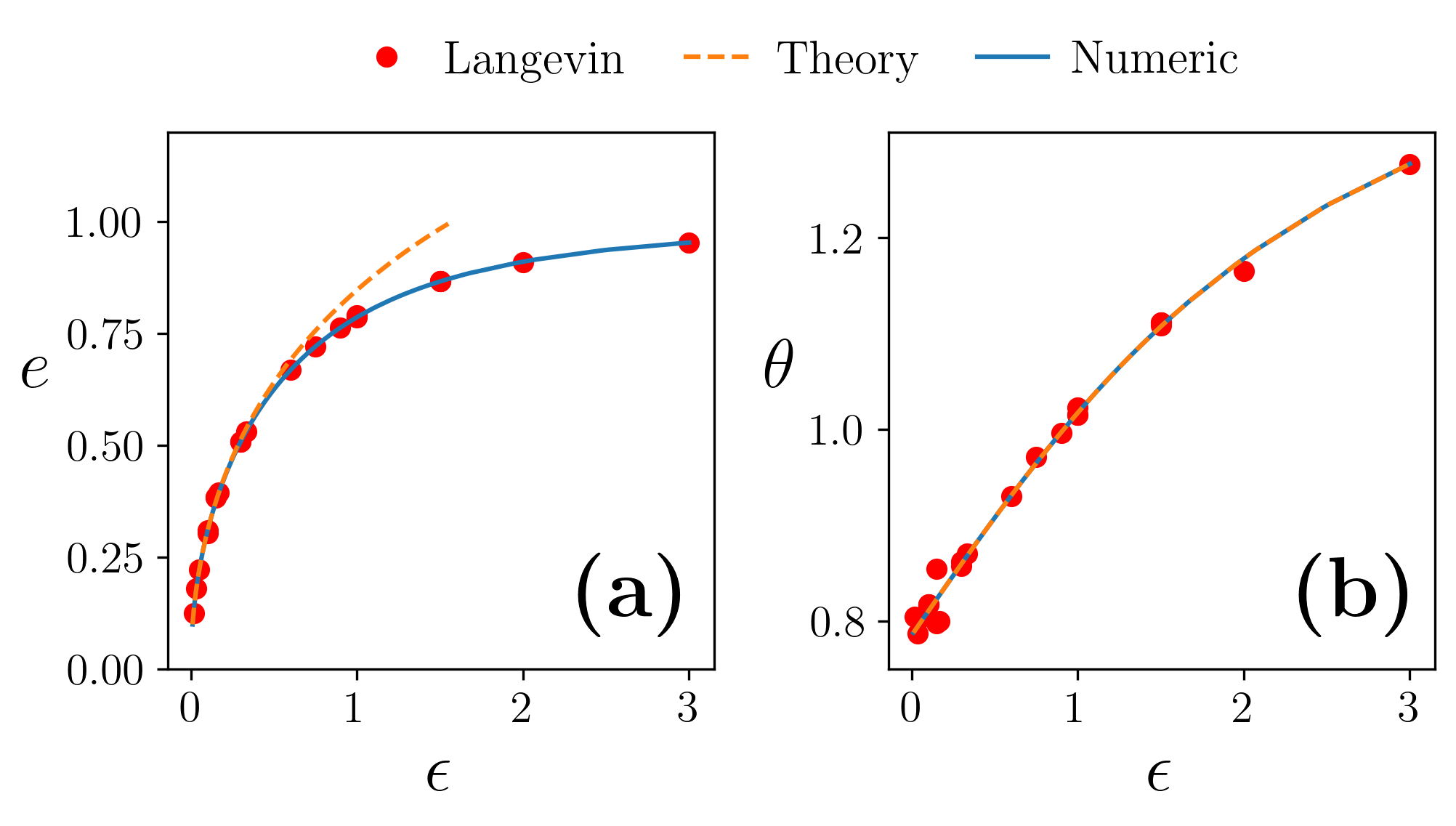
To test the accuracy of this method, we calculate a contour line (an ellipse) of thus computed , and plot its eccentricity and inclination angle , i.e., the angle between the major axis and the y-axis. The results are shown in Fig. 2 as the solid lines (Numeric). Also shown there are the corresponding results computed using direct simulation of the Langevin dynamics Eq. (2) (red dots, Langevin), as well as the analytical results given by Eqs. (27) (dashed lines, Theory). As one can see there, the numeric results agree with the Langevin results for all values of , which establishes the accuracy of the methods presented in App. A.1 for computation of and . By contrast, the analytical results are accurate only for small value of .
More numerical testings of our computation methods are supplied in App. A.1.
V.2 Verification of FTs
To verify FTs (90), we numerically simulate each of the four processes defined in Sec. III.3. We generate a large number of trajectories for each process, using the recipe discussed in App. A.3, compute the total work, the housekeeping work, and the excess work for each trajectory in each process, and thereby obtain the distributions of these works. The numerical method for computation of work at the trajectory level is explained in Appendix. A.4. In all simulations discussed here, . More simulations with different values of are presented in App. B.
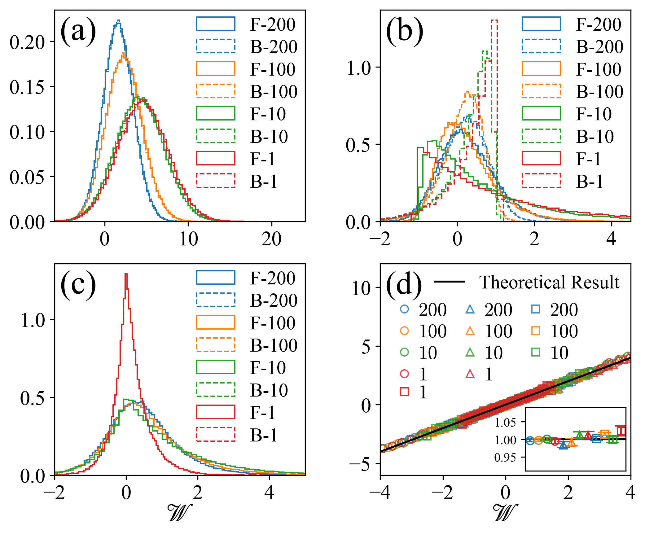
We first verify Eq. (90a), which may be rewritten as
| (105) |
| process | control parameters | duration | |
| (a) | 200, 100, 10, 1 | ||
| (b) | 0 | 200, 100, 10, 1 | |
| (c) | 0 | 200, 100, 10, 1 | |
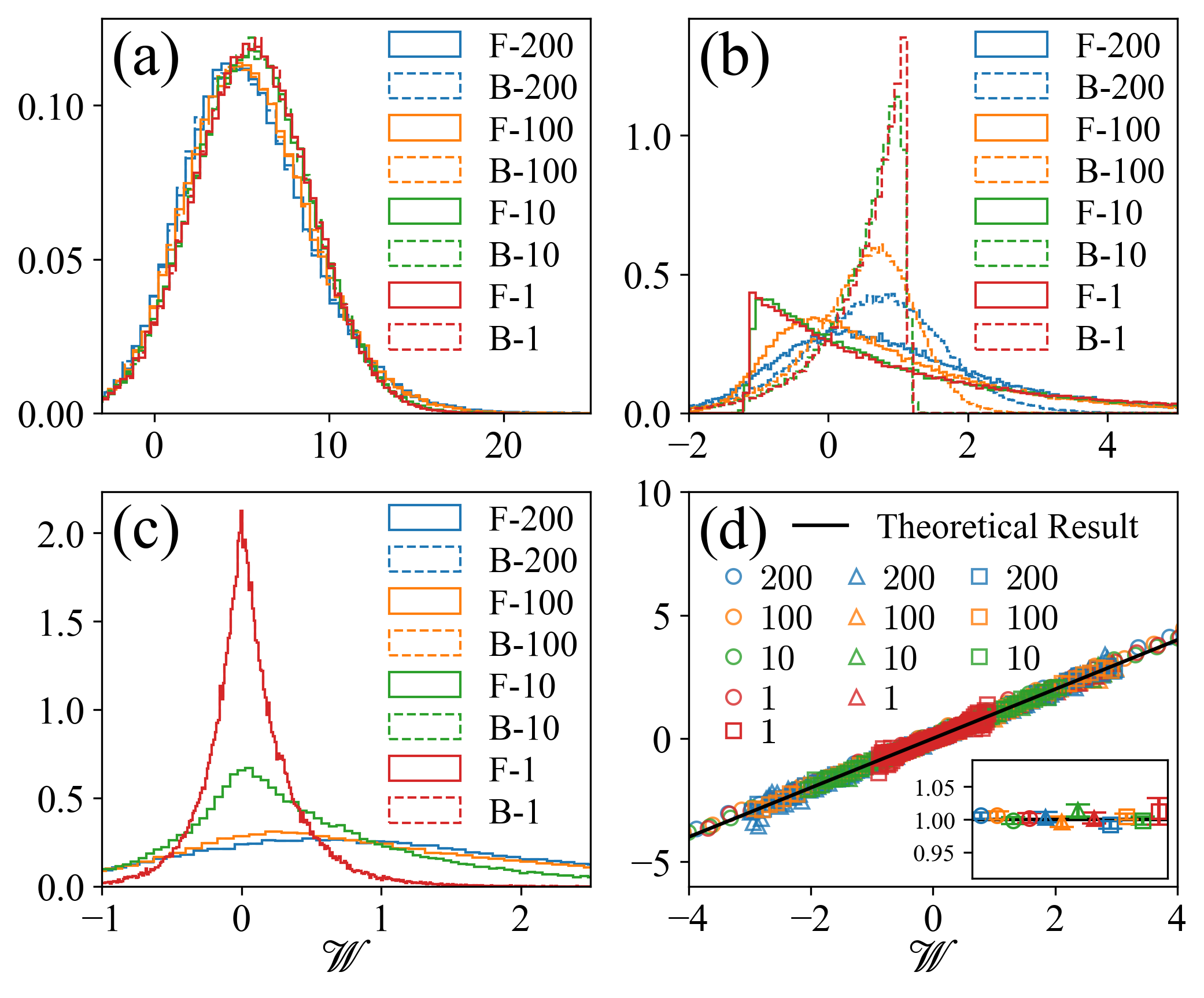
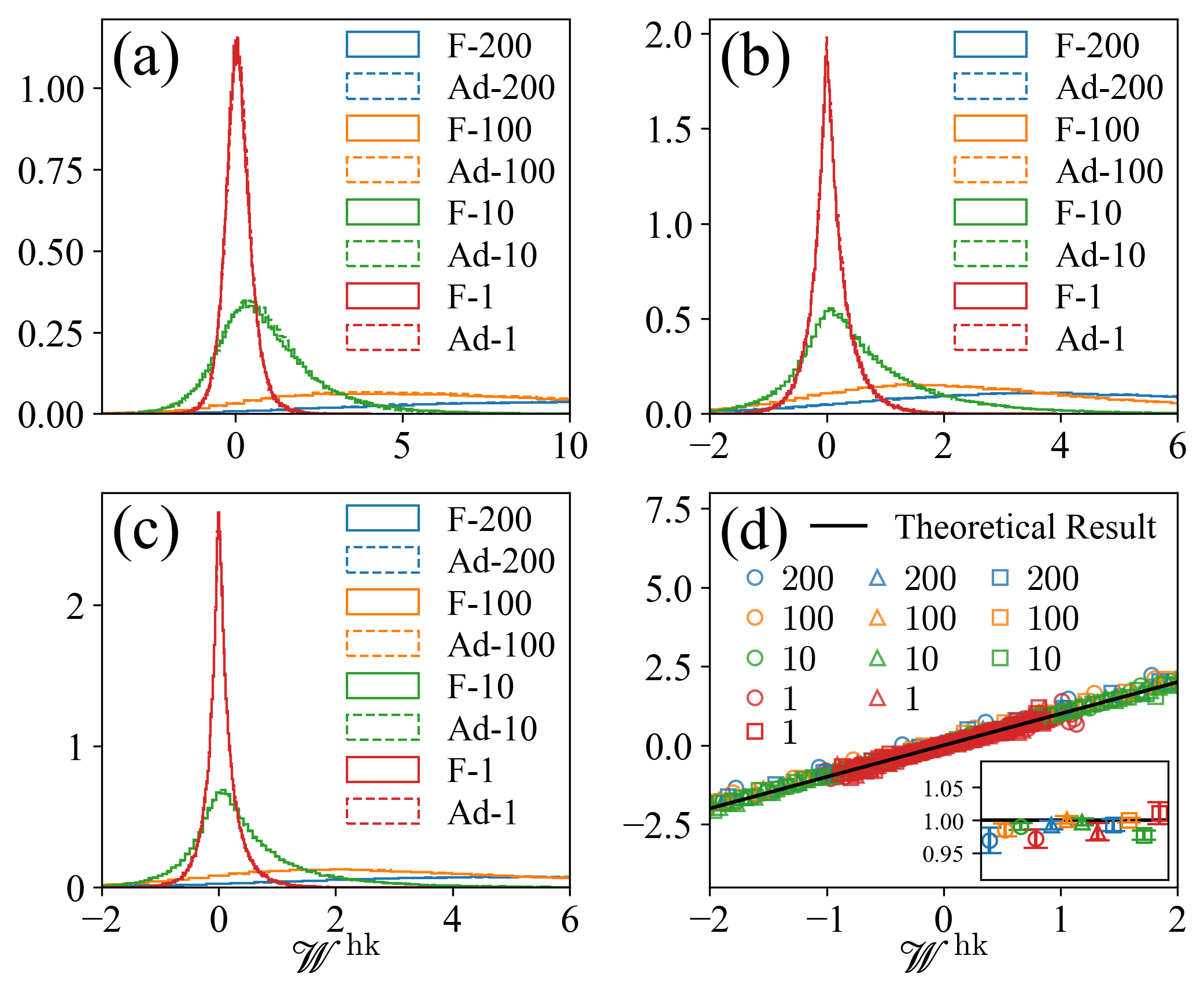
We simulate three processes that are shown in Table 2. The duration of each process is varied systematically, as shown in the last column of the table. For each protocol, we sample trajectories and compute the distribution of work. We then simulate the backward process, and compute the corresponding distribution of work. These work distributions are displayed in Fig. 3 (a), (b), and (c). Finally we use these distributions to verify the FT (105). As shown in Fig. 3 (d), all data collapse to the black straight-line as predicted by our theory.
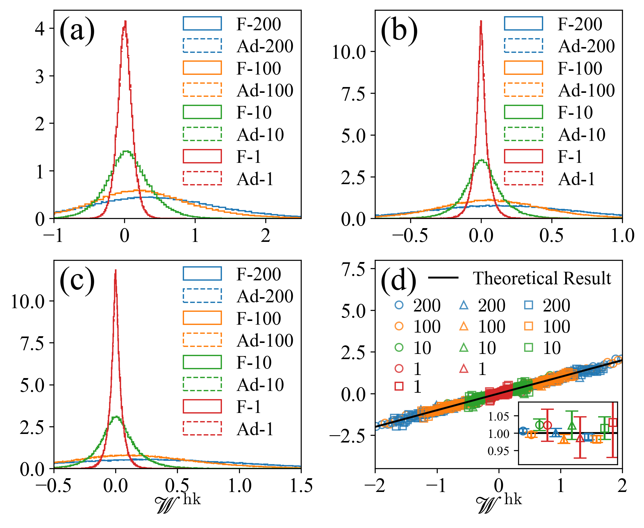
Now we verify Eq. (90b), which may be rewritten as
| (106) |
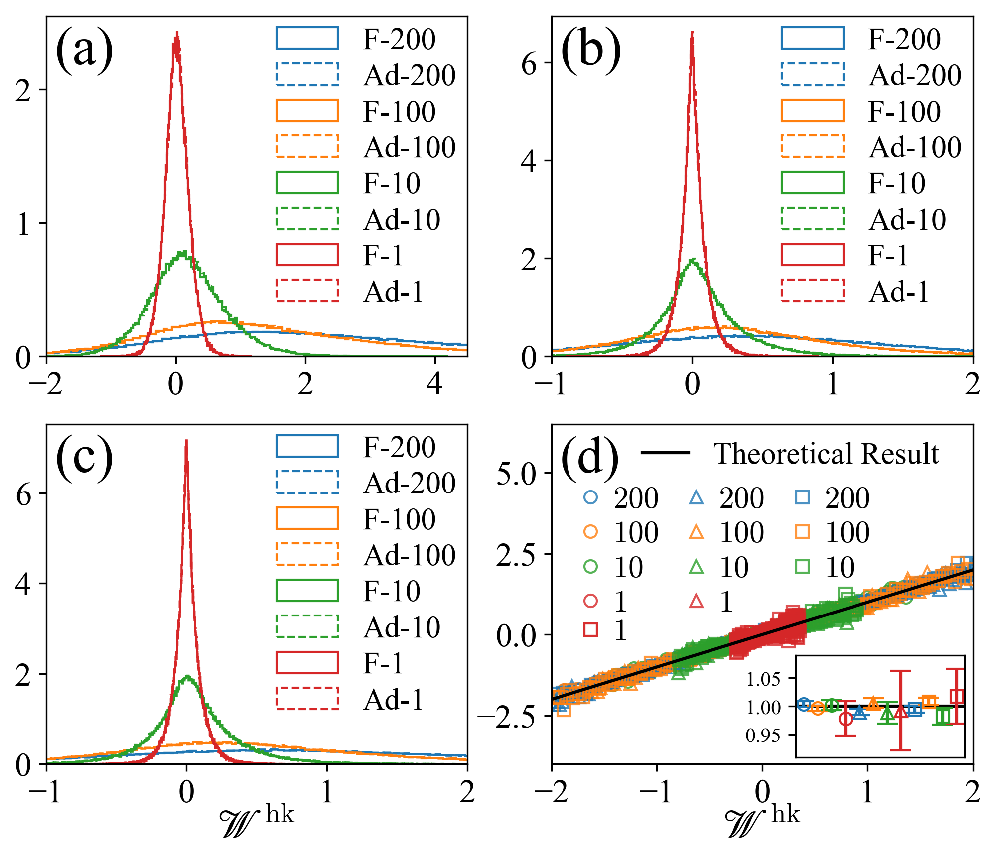
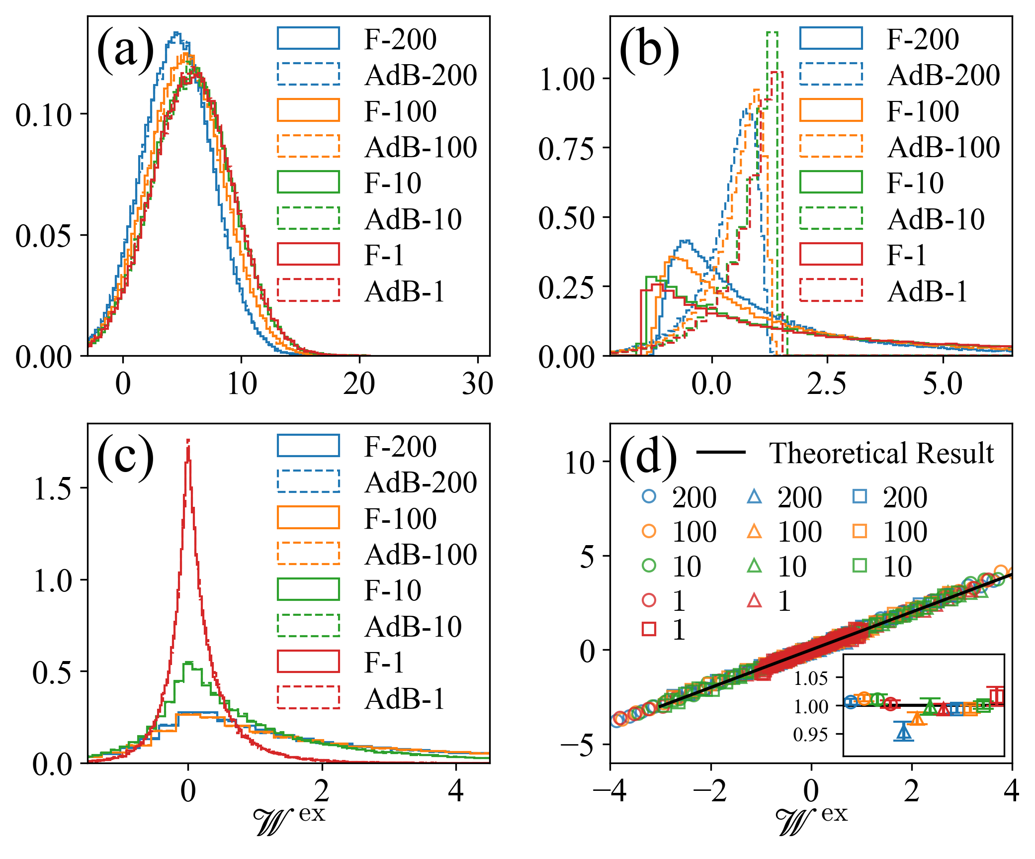
We simulate three types of forward processes that are shown in Table 3. The duration of each process is varied systematically, as shown in the last column of the table. For each protocol, we sample trajectories and compute the distribution of work. We then do the same for the adjoint processes. All work distributions are displayed in Fig. 4 (a), (b), and (c). Finally, we use these distributions to verify the FT (106). As shown in Fig. 4 (d), all data collapse to the black straight-line as predicted by our theory.
| process | control parameters | duration | |
| (a) | 0.01 | 200, 100, 10, 1 | |
| (b) | 0 | 200, 100, 10, 1 | |
| (c) | 0 | 200, 100, 10, 1 | |
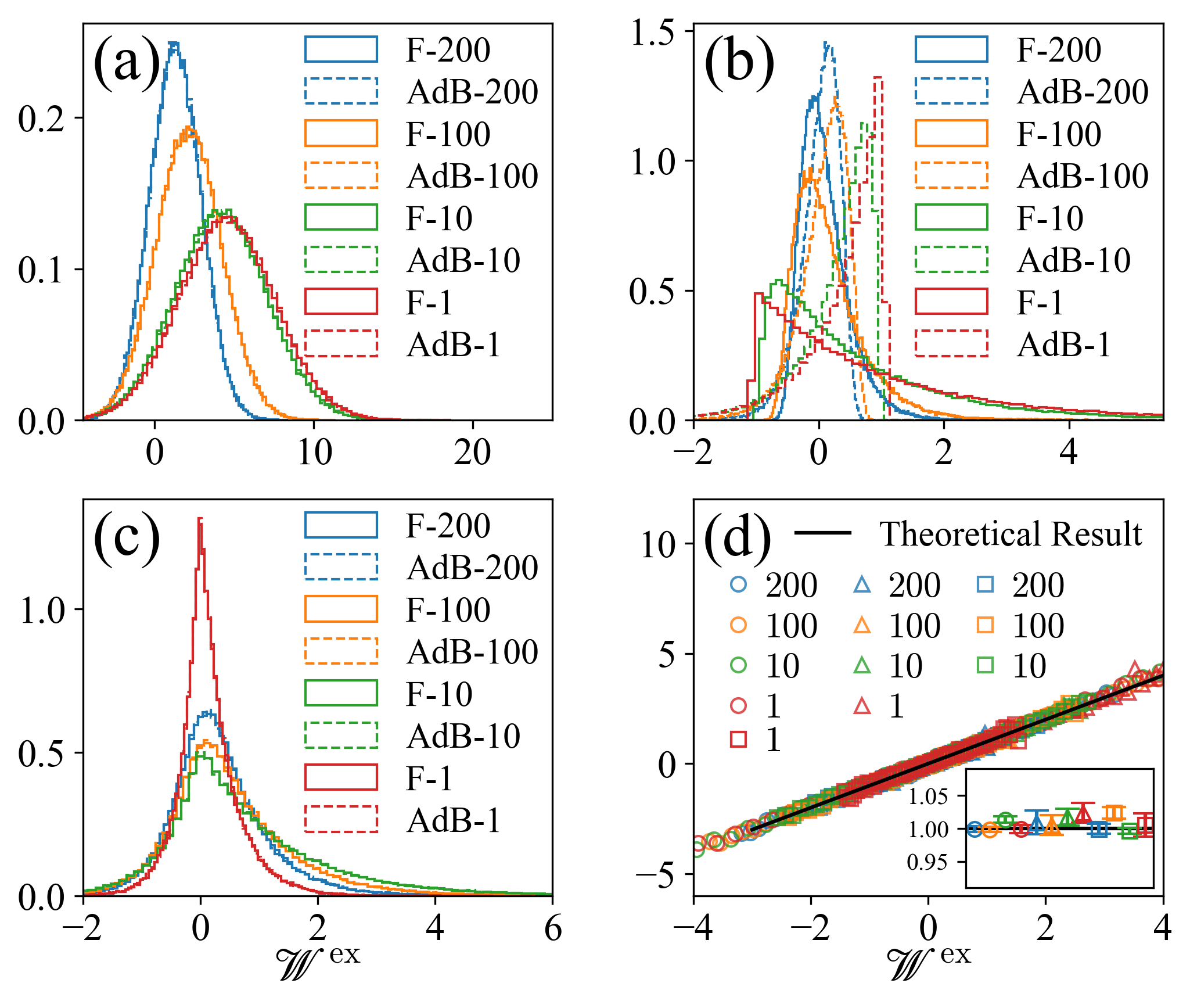
Now we verify Eq. (90c), which may be rewritten as
| (107) |
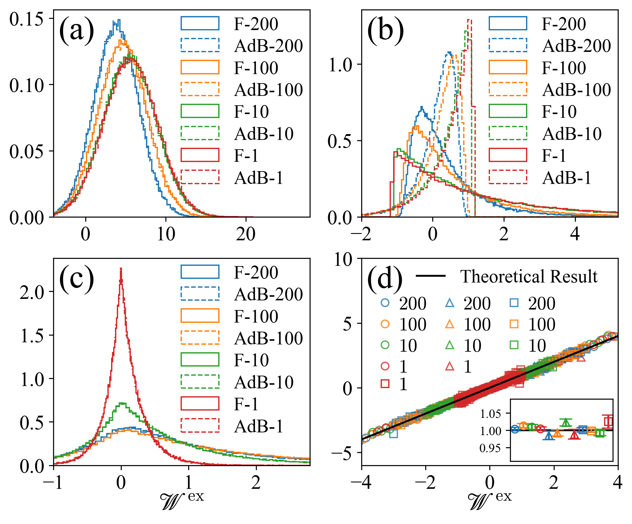
We simulate the same processes as shown in Table 2, and compute the distributions of excess work. We then do the same for the adjoint backward processes. All work distributions are displayed in Fig. 5 (a), (b), and (c). Finally, we use these distributions to verify the FT (107). As shown in Fig. 5 (d), all data collapse to the black straight-line as predicted by our theory.
VI Conclusion
In this work, we have developed a theory of stochastic thermodynamics for over-damped Brownian motion in a flowing fluid. To the best of our knowledge, this is the first concrete example of non-equilibrium small systems for which fluctuation theorems of the total work, the housekeeping work, and the excess work are explicitly established and verified. The analytic and numerical methods we employed here should be valuable for study of other non-equilibrium systems.
The authors acknowledge support from NSFC via grant #12375035, as well as Shanghai Municipal Science and Technology Major Project (Grant No.2019SHZDZX01).
References
- [1] Albert Einstein et al. On the motion of small particles suspended in liquids at rest required by the molecular-kinetic theory of heat. Annalen der physik, 17(549-560):208, 1905.
- [2] Robert Zwanzig. Nonequilibrium statistical mechanics. Oxford university press, 2001.
- [3] G. Gallavotti and E. G. D. Cohen. Dynamical Ensembles in Nonequilibrium Statistical Mechanics. Physical Review Letters, 74(14):2694–2697, April 1995.
- [4] Debra J. Searles and Denis J. Evans. Fluctuation theorem for stochastic systems. Physical Review E, 60(1):159–164, July 1999.
- [5] Udo Seifert. Stochastic thermodynamics, fluctuation theorems and molecular machines. Reports on Progress in Physics, 75(12):126001, December 2012.
- [6] Luca Peliti and Simone Pigolotti. Stochastic Thermodynamics: An Introduction. Princeton University Press, 2021.
- [7] Christian Van den Broeck et al. Stochastic thermodynamics: A brief introduction. Phys. Complex Colloids, 184:155–193, 2013.
- [8] Christopher Jarzynski. Equalities and Inequalities: Irreversibility and the Second Law of Thermodynamics at the Nanoscale. Annual Review of Condensed Matter Physics, 2(1):329–351, 2011.
- [9] Gavin E. Crooks. Entropy production fluctuation theorem and the nonequilibrium work relation for free energy differences. Physical Review E, 60(3):2721–2726, September 1999.
- [10] Thomas Speck, Jakob Mehl, and Udo Seifert. Role of External Flow and Frame Invariance in Stochastic Thermodynamics. Physical Review Letters, 100(17):178302, April 2008.
- [11] Minghao Li, Oussama Sentissi, Stefano Azzini, and Cyriaque Genet. Galilean relativity for Brownian dynamics and energetics. New Journal of Physics, 23(8):083012, August 2021.
- [12] Andrea Cairoli, Rainer Klages, and Adrian Baule. Weak Galilean invariance as a selection principle for coarse-grained diffusive models. Proceedings of the National Academy of Sciences, 115(22):5714–5719, May 2018.
- [13] Sascha Gerloff and Sabine H. L. Klapp. Stochastic thermodynamics of a confined colloidal suspension under shear flow. Physical Review E, 98(6):062619, December 2018.
- [14] Aishani Ghosal and Binny J. Cherayil. Polymer extension under flow: A path integral evaluation of the free energy change using the Jarzynski relation. The Journal of Chemical Physics, 144(21):214902, June 2016.
- [15] Asawari Pagare and Binny J. Cherayil. Stochastic thermodynamics of a harmonically trapped colloid in linear mixed flow. Physical Review E, 100(5):052124, November 2019.
- [16] Aishani Ghosal and Binny J Cherayil. Fluctuation relations for flow-driven trapped colloids and implications for related polymeric systems. THE EUROPEAN PHYSICAL JOURNAL B, 92:243, 2019.
- [17] Vladimir Y. Chernyak, Michael Chertkov, and Christopher Jarzynski. Path-integral analysis of fluctuation theorems for general Langevin processes. Journal of Statistical Mechanics: Theory and Experiment, 2006(08):P08001, August 2006.
- [18] Massimiliano Esposito and Christian Van den Broeck. Three Detailed Fluctuation Theorems. Physical Review Letters, 104(9):090601, March 2010.
- [19] Massimiliano Esposito and Christian Van den Broeck. Three faces of the second law. I. Master equation formulation. Physical Review E, 82(1):011143, July 2010.
- [20] Christian Van den Broeck and Massimiliano Esposito. Three faces of the second law. II. Fokker-Planck formulation. Physical Review E, 82(1):011144, July 2010.
- [21] Mingnan Ding, Fei Liu, and Xiangjun Xing. Unified theory of thermodynamics and stochastic thermodynamics for nonlinear Langevin systems driven by non-conservative forces. Physical Review Research, 4(4):043125, November 2022.
- [22] Mingnan Ding, Jun Wu, and Xiangjun Xing. Stochastic thermodynamics of Brownian motion in temperature gradient. Journal of Statistical Mechanics: Theory and Experiment, 2024(3):033203, March 2024.
- [23] Mingnan Ding and Xiangjun Xing. Time-Slicing Path-integral in Curved Space. Quantum, 6:694, April 2022.
- [24] E. H. Trepagnier, C. Jarzynski, F. Ritort, G. E. Crooks, C. J. Bustamante, and J. Liphardt. Experimental test of Hatano and Sasa’s nonequilibrium steady-state equality. Proceedings of the National Academy of Sciences, 101(42):15038–15041, October 2004.
- [25] Donghwan Yoo, Youngkyun Jung, and Chulan Kwon. Molecular dynamics on nonequilibrium motion of a colloidal particle driven by an external torque. Journal of Physics A: Mathematical and Theoretical, 50(10):105002, March 2017.
- [26] Peter E. Kloeden and Eckhard Platen. Stochastic Differential Equations, pages 103–160. Springer Berlin Heidelberg, Berlin, Heidelberg, 1992.
Appendix A The Numerical Methods
A.1 Computation of and
Here we explain how to compute the coefficients in the expansion Eq. (28). We consider slightly more general forms of quadratic confining potential and linear incompressible velocity field:
| (108) | |||||
| (109) |
Using Eq. (12), we may rewrite the Gibbs gauge condition (16) as
| (110) |
Note that the l.h.s. is also a quadratic form of .
We insert Eqs. (108), (109), and (28) into Eq. (110) and compare all coefficients of the quadratic form, we find following set of nonlinear equations:
| (111a) | ||||
| (111b) | ||||
| (111c) | ||||
| (111d) | ||||
| (111e) | ||||
| (111f) | ||||
Notice that only five of these equations are independent, since there are only five unknowns appearing in these equations.
A.2 Testing of numerical methods
Here we supply more testing of the analytic results (27) as well as the numerical results for , obtained using the method discussed in Eq. (A.1).
We simulate the Langevin dynamics (2) with the confine potential and flow field given by Eqs. (25), and compute the NESS pdf and probability current. We do the same thing for the adjoint dynamics, where the confining potential and the flow field are given by Eqs. (24).
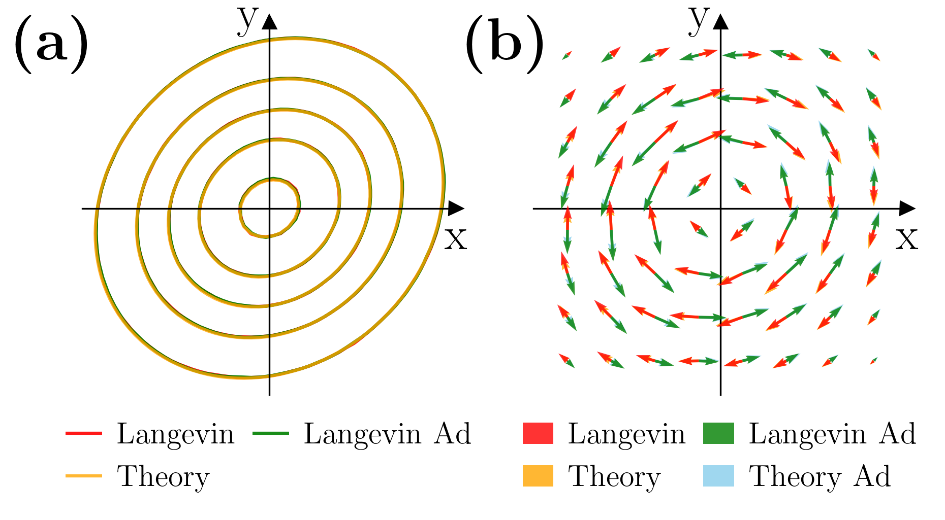
Firstly we let , so that the analytical results (27) are expected to be good.
In Fig. 6(a) we plot the contour lines of the NESS pdfs both for the original dynamics and the adjoint dynamics, computed using simulation data. In the same figure we also show the contour lines of the NESS pdf given by analytic results, i.e., Eqs. (13) and (27). As one can see there, all results agree with each other up to high precision.
In Fig. 6(b), we plot the NESS probability currents of both the original dynamics and the adjoint dynamics. As one can see, the probability current of the forward process is the opposite of that of the adjoint process. Additionally, theoretical results agree with numerical results.
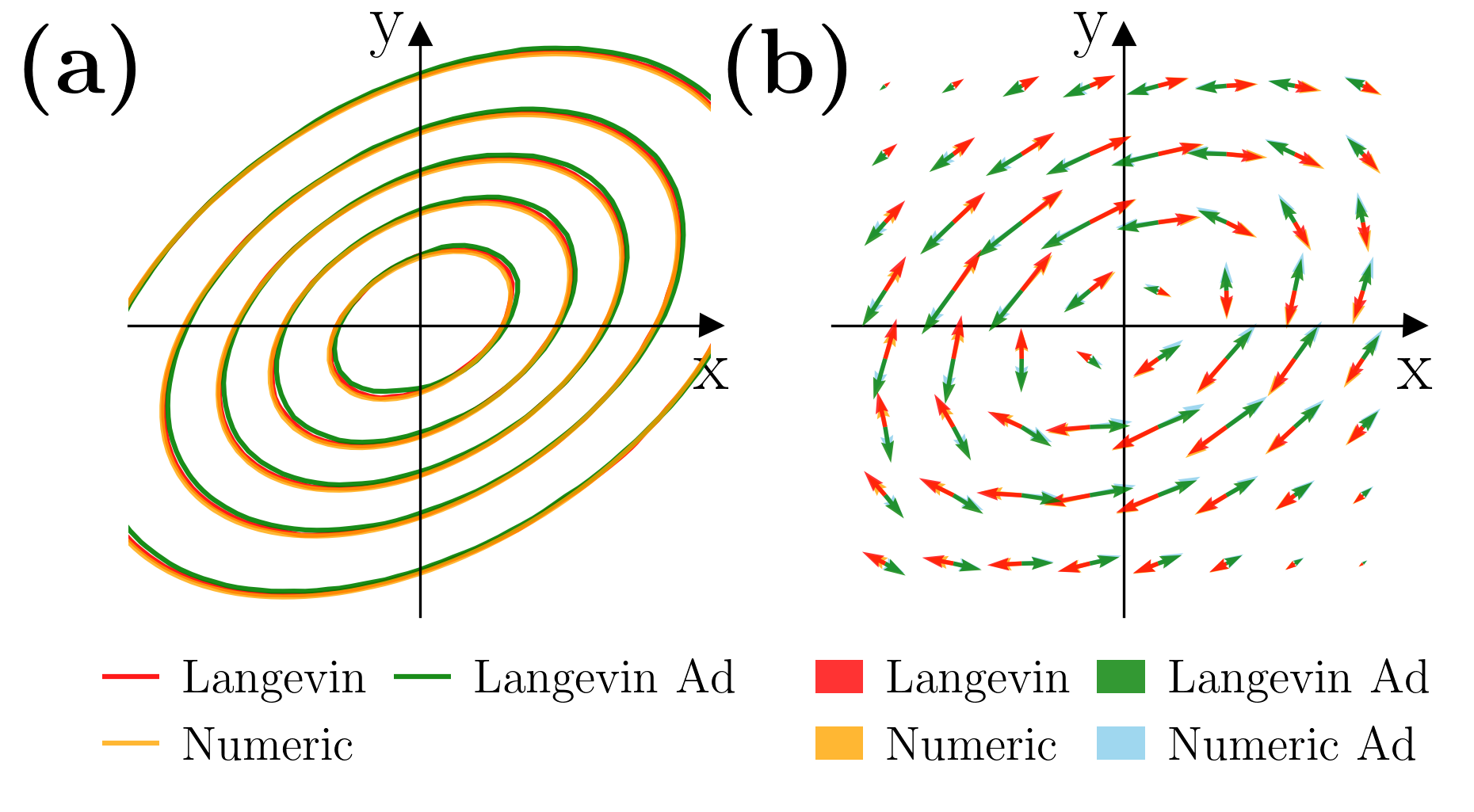
Now we let , so that the analytical results (27) are not expected to be good. We will then use the numerical method discussed in App. A.1 to compute .
In Fig. 7(a) we plot the contour lines of the NESS pdfs both for the original dynamics and the adjoint dynamics, computed using simulation data. In the same figure we also show the contour lines of the NESS pdf computed using the method discussed in App. A.1. As one can see there, all results agree with each other up to high precision.
In Fig. 7(b), we plot the NESS probability currents of both the original dynamics and the adjoint dynamics, computed both using direction simulation of the Langevin dynamics, and using the method discussed in App. A.1. As one can see, the probability current of the forward process is the opposite of that of the adjoint process. Additionally, simulation results agree with numerical results.
A.3 Numerical integration of Langevin dynamics
First we discretize with step size :
| (112) | |||||
| (113) | |||||
| (114) |
so that Eq. (2) is discretized as follows:
| (115) |
where is a 2d vector of normalized Gaussian random variables, and and are respectively the discretized force and fluid velocity:
| (116) | ||||
| (117) |
Note that the potential and the flow field are given in Eqs. (25).
We then numerically solve the discretized equations (115).
A.4 Calculation of Work
The total work along a trajectory is given in Eq. (74a). It can be discretized as
| (118) |
where is defined in Eq. (114), and is given in Eq.(28), whereas is defined as
| (119) |
It is important to evaluate at rather than any other place, in order to correctly compute the Stratonovich product in Eq. (74a).
The housekeeping work and excess work, defined in Eqs.(75a) can be similarly discretized:
| (120) | ||||
| (121) |
Appendix B FT with Other parameter
B.1 Small Shear Rate
In this part, we also verify FTs (90). In all simulations discussed here, we set parameter , and .
We first verify Eq. (90a), which may be rewritten as in Eq. (105). We simulate three processes that are shown in Table 2. The duration of each process is varied systematically, as shown in the last column of the table. For each protocol, we sample trajectories and compute the distribution of work. We then simulate the backward process, and compute the corresponding distribution of work. These work distributions are displayed in Fig. 8 (a), (b), and (c). Finally we use these distributions to verify the FT (105). As shown in Fig. 8 (d), all data collapse to the black straight-line as predicted by our theory.
Then we verify Eq. (90b), which may be rewritten as in Eq. (106). We simulate three types of forward processes that are shown in Table 3. The duration of each process is varied systematically, as shown in the last column of the table. For each protocol, we sample trajectories and compute the distribution of work. We then do the same for the adjoint processes. All work distributions are displayed in Fig. 9 (a), (b), and (c). Finally, we use these distributions to verify the FT (106). As shown in Fig. 9 (d), all data collapse to the black straight-line as predicted by our theory.
Finally we verify Eq. (90c), which may be rewritten as in Eq. (107). We simulate the same processes as shown in Table 2, and compute the distributions of excess work. We then do the same for the adjoint backward processes. All work distributions are displayed in Fig. 10 (a), (b), and (c). Finally, we use these distributions to verify the FT (107). As shown in Fig. 10 (d), all data collapse to the black straight-line as predicted by our theory.
B.2 Larger Shear Rate
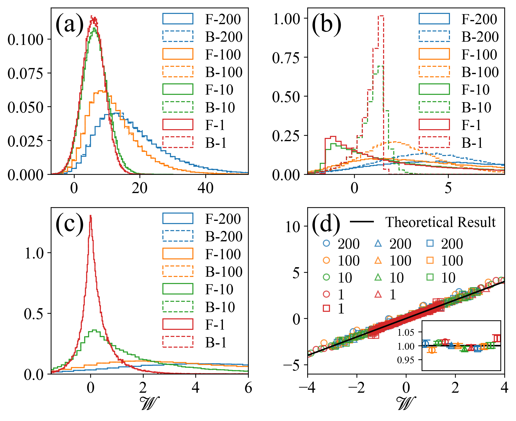
In this part, we also verify FTs (90). In all simulations discussed here, we set parameter , and .
We first verify Eq. (90a), which may be rewritten as in Eq. (105). We simulate three processes that are shown in Table 2. The duration of each process is varied systematically, as shown in the last column of the table. For each protocol, we sample trajectories and compute the distribution of work. We then simulate the backward process, and compute the corresponding distribution of work. These work distributions are displayed in Fig. 11 (a), (b), and (c). Finally we use these distributions to verify the FT (105). As shown in Fig. 11 (d), all data collapse to the black straight-line as predicted by our theory.
Then we verify Eq. (90b), which may be rewritten as in Eq. (106). We simulate three types of forward processes that are shown in Table 3. The duration of each process is varied systematically, as shown in the last column of the table. For each protocol, we sample trajectories and compute the distribution of work. We then do the same for the adjoint processes. All work distributions are displayed in Fig. 12 (a), (b), and (c). Finally, we use these distributions to verify the FT (106). As shown in Fig. 12 (d), all data collapse to the black straight-line as predicted by our theory.
Finally we verify Eq. (90c), which may be rewritten as in Eq. (107). We simulate the same processes as shown in Table 2, and compute the distributions of excess work. We then do the same for the adjoint backward processes. All work distributions are displayed in Fig. 13 (a), (b), and (c). Finally, we use these distributions to verify the FT (107). As shown in Fig. 13 (d), all data collapse to the black straight-line as predicted by our theory.