Stock loan with Automatic termination clause, cap and margin

Shuqing Jiang
Department of Mathematical Sciences, Tsinghua University, Beijing 100084, China. Email: jiangsq06@gmail.com
Zongxia Liang
Department of Mathematical Sciences, Tsinghua University, Beijing 100084, China. Email: zliang@math.tsinghua.edu.cn
Weiming Wu
Department of Mathematical Sciences, Tsinghua University, Beijing 100084, China. Email: wuweiming03@gmail.com

Abstract.

This paper works out fair values of stock loan model with automatic termination clause, cap and margin. This stock loan is treated as a generalized perpetual American option with possibly negative interest rate and some constraints. Since it helps a bank to control the risk, the banks charge less service fees compared to stock loans without any constraints. The automatic termination clause, cap and margin are in fact a stop order set by the bank. Mathematically, it is a kind of optimal stopping problems arising from the pricing of financial products which is first revealed. We aim at establishing explicitly the value of such a loan and ranges of fair values of key parameters : this loan size, interest rate, cap, margin and fee for providing such a service and quantity of this automatic termination clause and relationships among these parameters as well as the optimal exercise times. We present numerical results and make analysis about the model parameters and how they impact on value of stock loan. MSC(2000): primary 91B24, 91B28,91B70 secondary 60H05, 60H10 Keywords: Stock loan model; Automatic termination clause; Optimal stopping problem; Perpetual American option; Black-Scholes model.

1. Introduction

A stock loan is a popular financial product provided by many banks and financial institutions in which a client (borrower), who owns one share of stock, borrows a loan of amount $q$ from a bank (lender) with the share of stock as collateral, and the bank receives amount $c$ from the client as the service fee. The client may regain the stock by repaying the principal and interest (that is, $qe^{\gamma t}$ , where $\gamma$ is continuously compounding loan interest rate ) to the bank at any time $t$ , or surrender the stock instead of repaying the loan. The key point of making the stock loan contract is to find values of the parameters $q$ , $c$ , and $\gamma$ . The stock loan has many advantages for the client. It creates liquidity while overcoming the barrier of large block sales, such as triggering tax events or controlling restrictions on sales of stocks. It also serves as a hedge against a market down turn : if the stock price goes down, the client may just forfeit the stock and does not repay the loan; if however the stock price goes up, the client keeps all the benefits upside by repaying the principal and interest. In other words, a stock loan can help high-net-worth investors with large equity positions to achieve a variety of objectives.

The stock loan valuation is essentially a kind of optimal stopping problems. A typical and well-known example of optimal stopping problems is the American option. There are many literatures about the American option, we refer the readers to Hull [20], Gerber and Shiu [17] and Broadie and Detemple [8], Jiang [21], Detemple et al. [13], Cheuk and Vorst [9], Windcliff et al. [36], and Dai et al. [10]. Stock loan valuation has attracted much interest of both academic researchers and financial institution recently. Xia and Zhou [37] first studied the problem of stock loan under the Black-Scholes framework. They established stock loan model and got its valuation by a pure probabilistic approach. They also pointed out that variational inequality approach can not be directly applied to these kinds of stock loans. Zhang and Zhou [38] used the variational inequality approach to solve the stock loan pricing problem treated in[37], and they carried the approach over to the models in which the underlying stock price follows a geometric Brownian motion with regime switching(cf.[38]). Dai and Xu [11]considered the valuation of stock loan that the accumulative dividends may be gained by the borrower or the lender according to the provision of the loan.

In order to control effectively the risk and make the stock loan contract worthwhile so that it can provide the writer with protection, the bank and client embed an automatic termination clause, cap $L$ and margin $k$ into the stock loan. The stock loan can then be terminated via the clause when the share price is too low, that is, the automatic termination clause is triggered if and only if the discounted stock price is less than $a$ (i.e., $e^{-\gamma t}S_{t}\leq a$ ). Since it helps a bank to control the risk, the bank should charge less service fee initially compared to the stock loan without the automatic termination clause. The bank will terminate a stock loan contract by acquiring the ownership of the collateral equity and the client will not need to pay the principle and interest when the automatic termination clause is triggered at time $t$ . Hence, the client can choose to regain the stock by repaying the loan principal and interest. The automatic termination clause can be described by a quantity $a$ $(0<a\leq q)$ , which is also a key point of negotiation between the bank and the client. Because there is a distinction between what is actuarial fair value and values as the solution of a mathematical problem, we need to determine the fair value of this loan, ranges of fair values of the parameters $(q,\gamma,c,a,L,k)$ and relationships among these parameters in some reasonable sense so that the client and the bank know whether this actuarial value is reasonable( that is, this value belongs to the ranges and satisfies the relationships). Therefore, working out this value in this contract will be a main task in negotiation between the client and the bank initially. Thus this is a problem of theoretical value finding as well as practical implication for option pricing. To the best of our knowledge, there are a few results on this topic have been reported, we refer the readers to Dai and Xu [11], Liu and Xu [18], Xia and Zhou[37] and Zhang and Zhou[38]. The main purpose of the present paper is to determine the right values of these parameters $(q,\gamma,c,a,L,K)$ : the principal $q$ , the interest rate $\gamma$ , the fee $c$ charged by the bank, the barrier $a$ , the cap $L$ and margin $k$ in the stock loan contract with automatic termination clause and find relationships among these parameters by deriving optimal exercise time (stopping time) and valuation formulas of the stock loan under the assumption $\delta>0$ and $\gamma-r+\delta\geq 0$ or $\delta=0$ and $\gamma-r>\frac{\sigma^{2}}{2}$ ( where $\delta$ is the dividend yield, $r$ is the risk-free rate, and $\sigma$ is the volatility). We try to develop variational inequality method(cf. [23, 31, 29]) with probabilistic approach to deal with this value of such a loan and ranges of fair values of this stock loan size, interest rate, cap, margin and fee for providing such a service and quantity of this automatic termination clause and relationships among these parameters. The paper establishes a general setting to broaden the applicability of our method concerning different stock loans.

The paper is organized as following: In section 2, we formulate a mathematical model of the stock loan with automatic termination clause. In section 3, we evaluate the stock loan by variational inequality method and obtain an optimal exercise time. In section 4, we derive probabilistic solutions and terminable exercise times of the stock loan. In section 5,we study a mathematical model of the stock loan with automatic termination clause, cap and margin by applying the way we used in the section 3 and section 4 to determine fair values of the stock loan in section 6. In section 7 we give some numerical results of two stock loans. In section 8, we give an over view of the main findings in this paper. In appendix, we further give discussions of the parameters.

2. Formulation of stock loan with automatic termination clause

We introduce in this section the standard Black-Scholes model in a continuous-time financial market consisting of two assets: a risky asset stock $S$ and a locally risk-less money account $B\equiv\{B_{t},t\geq 0\}$ . The uncertainty is described by a standard Brownian motion $\mathcal{W}\equiv\{\mathcal{W}_{t},t\geq 0\}$ defined on a risk-neutral probability space $(\Omega,\mathcal{F},\{\mathcal{F}_{t}\}_{t\geq 0},P)$ , where $\{\mathcal{F}_{t}\}_{t\geq 0}$ is the $P-$ augmentation of the filtration generated by $\mathcal{W}$ , with $\mathcal{F}_{0}=\sigma\{\Omega,\emptyset\}$ and $\mathcal{F}=\sigma\{\bigcup_{t\geq 0}\mathcal{F}_{t}\}$ . The terms fair value, right value and proper value, $\cdots$ in this paper mean that they are determined under this risk-neutral probability $P$ . The locally risk-less money account $B$ evolves according to the following dynamic system,

\displaystyle dB_{t}=rB_{t}dt,\ \ r>0.

The market price process $S$ of the stock follows a geometric Brownian motion,

\displaystyle S_{t}=S_{0}e^{(r-\delta-\frac{\sigma^{2}}{2})t+\sigma\mathcal{W}_{t}},

(2.1)

where $S_{0}$ is the initial stock price, $\delta\geq 0$ is the dividend yield and $\sigma>0$ is the volatility.

We now explain the stock loan (i.e., the contract) with an automatic termination clause in this paper as follows:

$\bullet$ At the beginning, a client borrows amount $q(q>0)$ from a bank with one share of stock as the collateral, and gives the bank amount $c(0\leq c\leq q)$ as the service fee. As a result, the client gets amount $q-c$ from the bank.

$\bullet$ The client has the option to regain the stock by paying amount $qe^{\gamma t}$ ( where $\gamma$ is the continuously compounding loan interest rate) to the bank (lender) at any time $t$ , or just gives the stock to the bank without repaying the loan before triggering the automatic termination clause. Dividends of the stock are collected by the bank until the client regains the stock, the dividends are not credited to the client.

$\bullet$ The client has no obligation to regain the stock whether the automatic termination clause is triggered or not. If the automatic termination clause is triggered, then the bank acquires the collateral stock, the contract is terminated, and the client loses the option to regain the stock.

$\bullet$ The values of $(q,\gamma,c,a)$ : the principal $q$ , the interest rate $\gamma$ , the fee $c$ charged by the bank, and the barrier $a$ are specified before this contract is exercised.

Xia and Zhou [37] established a stock loan without an automatic termination clause by probabilistic approach. They proved that the optimal exercise time is a hitting time:

\displaystyle\tau_{b}=\inf{\{t\geq 0,e^{-\gamma t}S_{t}\geq b\}},

then determined the value by maximizing expected discounted payoff of this stock loan given by $\tau_{b}$ for some $b\geq q\vee S_{0}$ , where $q$ is the principal of the stock loan and $S_{0}$ is the initial stock price.

The automatic termination clause is one of our main interest. The main goal of sections 3 and 4 is to determine fair value $f(S_{0})$ ( see (2.2) below) of the stock loan with an automatic termination clause and ranges of fair values of the parameters $(q,c,\gamma,a)$ under the assumption $\delta>0$ and $\gamma-r+\delta\geq 0$ or $\delta=0$ and $\gamma-r>\frac{\sigma^{2}}{2}$ (see Proposition 4.1 below). This problem can be treated as a generalized perpetual American option with a client initially buying at price $S_{0}-q+c$ .

We consider the automatic termination clause as follows: if the stock price satisfies $e^{-\gamma t}S_{t}\leq a,0<a\leq q$ ( $\gamma$ is the loan interest rate), then this stock loan is terminated. So the discounted payoff of this American contingent claim at stopping time $\tau\in\mathcal{T}_{0}$ is

\displaystyle Y(\tau)=e^{-r\tau}(S_{\tau}-qe^{\gamma\tau})_{+}I_{\{\tau<\tau_{a}\}},

where $\tau_{a}=\inf{\{t\geq 0,e^{-\gamma t}S_{t}\leq a\}}$ and $\mathcal{T}_{0}$ denotes all $\{\mathcal{F}_{t}\}_{t\geq 0}$ -stopping times. The initial value of this American contingent claim is the following (cf. [23, 34]),

$\displaystyle f(x)$	$\displaystyle=$	$\displaystyle\sup\limits_{\tau\in\mathcal{T}_{0}}{\bf E}\big{[}Y(\tau)\big{]}$	(2.2)
	$\displaystyle=$	$\displaystyle\sup\limits_{\tau\in\mathcal{T}_{0}}{\bf E}\big{[}e^{-r\tau}(S_{\tau}-qe^{\gamma\tau})_{+}I_{\{\tau<\tau_{a}\}}\big{]}$
	$\displaystyle=$	$\displaystyle\sup\limits_{\tau\in\mathcal{T}_{0}}{\bf E}\big{[}e^{-\tilde{r}\tau}(\tilde{S}_{\tau}-q)_{+}I_{\{\tau<\tau_{a}\}}\big{]},$

where $\tilde{r}=r-\gamma\leq 0$ and $\tilde{S}_{t}=e^{-\gamma t}S_{t},\tilde{S}_{0}=S_{0}=x$ . The value of this American contingent claim at time $t$ is the following,

\displaystyle V_{t}=\sup\limits_{\tau\in\mathcal{T}_{t}}{\bf E}\big{[}e^{-{r}(\tau-t)}(S_{\tau}-qe^{\gamma\tau})_{+}I_{\{\tau<\tau_{a}\}}|\mathcal{F}_{t}\big{]},

(2.3)

i.e.,

\displaystyle e^{-rt}V_{t}=\sup\limits_{\tau\in\mathcal{T}_{t}}{\bf E}\big{[}e^{-\tilde{r}\tau}(\tilde{S}_{\tau}-q)_{+}I_{\{\tau<\tau_{a}\}}|\mathcal{F}_{t}\big{]},

where $\mathcal{T}_{t}$ denotes all $\{\mathcal{F}_{t}\}_{t\geq 0}$ -stopping times $\tau$ with $\tau\geq t$ a.s..

In the following sections we first determine fair value $f(S_{0})$ of the stock loan with an automatic termination clause, then find ranges of fair values of the parameters $(q,c,\gamma,a)$ and relationships among these parameters by $f(S_{0})$ and equality $f(S_{0})=S_{0}-q+c$ .

3. Variational inequality method

In this section we compute the fair value $f(S_{0})$ of the stock loan with an automatic termination clause treated as a generalized perpetual American option with automatic termination clause. Note that since the payoff process of the option $Y(t)\geq 0$ a.s., and $Y(t)>0$ with a positive probability if $S_{0}>a$ , $Y(t)=0$ a.s. if $S_{0}\leq a$ , to avoid arbitrage we assume that

\displaystyle S_{0}-q+c>0,\ S_{0}>a,

(3.1)

and

\displaystyle S_{0}-q+c=0,\ S_{0}\leq a.

(3.2)

Now we introduce some quantitative properties on $f$ defined via (2.2) and solve the optimal stopping time problem (2.2) by variational method and stopping time techniques.

Proposition 3.1.

$(x-q)_{+}\leq f(x)\leq x$ for all $x\geq 0$ .

Proof.

By taking $\tau=0$ in (2.2) and noticing that $\tau<\tau_{a}$ , a.s., it is easy to see that $(x-q)_{+}\leq f(x)$ . As for the second inequality, we have

$\displaystyle f(x)$	$\displaystyle=$	$\displaystyle\sup\limits_{\tau\in\mathcal{T}_{0}}{\bf E}\big{[}e^{-\tilde{r}\tau}(\tilde{S}_{\tau}-q)_{+}I_{\{\tau<\tau_{a}\}}\big{]}$
	$\displaystyle\leq$	$\displaystyle\sup\limits_{\tau\in\mathcal{T}_{0}}{\bf E}\big{[}e^{-\tilde{r}\tau}\tilde{S}_{\tau}I_{\{\tau<\tau_{a}\}}\big{]}$
	$\displaystyle\leq$	$\displaystyle\sup\limits_{\tau\in\mathcal{T}_{0}}{\bf E}\big{[}e^{-\tilde{r}(\tau\wedge\tau_{a})}\tilde{S}_{\tau\wedge\tau_{a}}\big{]}$
	$\displaystyle=$	$\displaystyle\sup\limits_{\tau\in\mathcal{T}_{0}}{\bf E}\big{[}xe^{\sigma\mathcal{W}_{\tau\wedge\tau_{a}}-\frac{\sigma^{2}}{2}\tau\wedge\tau_{a}}\big{]}$
	$\displaystyle=$	$\displaystyle x,$

where the last equality follows from the optional sampling theorem and the process $\{e^{\sigma\mathcal{W}_{t}-\frac{\sigma^{2}t}{{2}}},t\geq 0\}$ is a strong martingale. ∎

Remark 3.1.

It is easy to see from the definition of $f(x)$ that $f(x)$ is continuous, convex and nondecreasing with respect to $x$ .

Because the loan rate $\gamma$ is always greater than risk-free rate $r$ , our problem reduces to a generalized perpetual American contingent claim with possibly negative interest rate $r-\gamma$ , where the term negative interest rate is just used to state relationship between the model treated in this paper and an American perpetual call option with a time-varying striking price, and has no other implications. We have the following.

Theorem 3.1.

Assume that $\delta>0$ and $\gamma-r+\delta\geq 0$ or $\delta=0$ and $\gamma-r>\frac{\sigma^{2}}{2}$ . If $f(x)$ is continuous, $f(x)\in\mathcal{C}^{1}[(0,\infty)\setminus\{a\}]\cap\mathcal{C}^{2}[(0,\infty)\setminus\{a,b\}]$ for some $b\geq 0$ which we will discuss later, and $f(x)$ satisfies the following variational problem

\displaystyle\left\{\begin{array}[]{l l}\max{\{\frac{1}{2}\sigma^{2}x^{2}f^{{}^{\prime\prime}}+(\tilde{r}-\delta)xf^{{}^{\prime}}-\tilde{r}f,(x-q)_{+}-f\}}=0,x>a,\\ f(x)=0,x\leq a,\end{array}\right.

(3.5)

then $f(x)$ must be the function defined by (2.2 ) and $\tau_{b}=\inf{\{t\geq 0:e^{-\gamma t}S_{t}\geq b\}}$ attains the supremum in (2.2), i.e., $\tau_{b}$ is optimal.

Remark 3.2.

The value $a$ is always determined by negotiation between the bank and the client initially, the $b$ is an endogenous parameter to be determined late in this model.

Proof.

Let $f(x)$ satisfy problem (3.5), we want to show that $f$ must be the function defined by (2.2). Since $f(x)=0$ , $0<x\leq a$ , we only need to prove Theorem 3.1 in the region $a<x$ . We will prove Theorem 3.1 in two steps.
Step one. We show that for any stopping time $\tau$

\displaystyle f(x)\geq{\bf E}\big{[}e^{-\tilde{r}\tau}(\tilde{S}_{\tau}-q)_{+}I_{\{\tau<\tau_{a}\}}\big{]}.

(3.6)

Applying Itô formula to convex function $f$ and the process $\tilde{S}_{t}$ defined in (2.2) and using (3.5)we have

	$\displaystyle d(e^{-\tilde{r}t}f(\tilde{S}_{t}))$	$\displaystyle=$	$\displaystyle e^{-\tilde{r}t}\tilde{S}_{t}f^{{}^{\prime}}(\tilde{S}_{t})\sigma d\mathcal{W}(t)-e^{-\tilde{r}t}\big{[}(\delta\tilde{S}_{t}-\tilde{r}q)I_{\{\tilde{S}_{t}>b\}}\big{]}dt$		(3.7)
		$\displaystyle\equiv$	$\displaystyle d\mathcal{M}(t)-d\Lambda(t),$		(3.7)

where

\displaystyle\mathcal{M}(t)\equiv\int_{0}^{t}e^{-\tilde{r}u}\tilde{S}_{u}f^{{}^{\prime}}(\tilde{S}_{u})\sigma d\mathcal{W}(u)

is a martingale, and

\displaystyle\Lambda(t)\equiv\int_{0}^{t}e^{-\tilde{r}u}[(\delta\tilde{S}_{u}-\tilde{r}q)I_{\{\tilde{S}_{u}>b\}}]du

is a nonnegative and nondecreasing process because $\delta x-\tilde{r}q\geq 0,x>b$ with $b>q\geq\frac{r-\gamma}{\delta}q$ under the assumption $\delta>0$ and $\gamma-r+\delta\geq 0$ , and $\tilde{r}=r-\gamma<0$ under the assumption $\delta=0$ and $\gamma-r>\frac{\sigma^{2}}{2}$ .

For any stopping time $\tau$ and any $t\in[0,\infty)$ , by (3.5), (3.7) and Proposition 3.1 we have

$\displaystyle f(\tilde{S}_{0})$	$\displaystyle=$	$\displaystyle{\bf E}\big{[}e^{-\tilde{r}(\tau\wedge\tau_{a}\wedge t)}f(\tilde{S}_{\tau\wedge\tau_{a}\wedge t})\big{]}+{\bf E}\big{[}\Lambda(\tau\wedge\tau_{a}\wedge t)\big{]}$	(3.8)
	$\displaystyle\geq$	$\displaystyle{\bf E}\big{[}e^{-\tilde{r}(\tau\wedge\tau_{a}\wedge t)}f(\tilde{S}_{\tau\wedge\tau_{a}\wedge t})\big{]}$
	$\displaystyle=$	$\displaystyle{\bf E}\big{[}e^{-\tilde{r}(\tau\wedge t)}f(\tilde{S}_{\tau\wedge t})I_{\{\tau<\tau_{a}\}}\big{]}+{\bf E}\big{[}e^{-\tilde{r}(\tau_{a}\wedge t)}f(\tilde{S}_{\tau_{a}\wedge t})I_{\{\tau_{a}\leq\tau\}}\big{]}$
	$\displaystyle\geq$	$\displaystyle{\bf E}\big{[}e^{-\tilde{r}(\tau\wedge t)}(\tilde{S}_{\tau\wedge t}-q)_{+}I_{\{\tau<\tau_{a}\}}\big{]}+{\bf E}\big{[}e^{-\tilde{r}(\tau_{a}\wedge t)}f(\tilde{S}_{\tau_{a}\wedge t})I_{\{\tau_{a}\leq\tau\}}\big{]}$
	$\displaystyle=$	$\displaystyle{\bf E}\big{[}e^{-\tilde{r}(\tau\wedge t)}(\tilde{S}_{\tau\wedge t}-q)_{+}I_{\{\tau<\tau_{a}\}}\big{]}+{\bf E}\big{[}e^{-\tilde{r}t}f(\tilde{S}_{t})I_{\{\tau_{a}\leq\tau\}}I_{\{\tau_{a}>t\}}\big{]},$

where we have used $f(\tilde{S}_{\tau_{a}})=0$ .

Obviously,

\displaystyle e^{-\tilde{r}(\tau\wedge t)}(\tilde{S}_{\tau\wedge t}-q)_{+}I_{\{\tau<\tau_{a}\}}\leq\sup\limits_{0\leq t<\infty}e^{-\tilde{r}t}(\tilde{S}_{t}-q)_{+}

and

\displaystyle e^{-\tilde{r}(\tau_{a}\wedge t)}f(\tilde{S}_{\tau_{a}\wedge t})I_{\{\tau_{a}\leq\tau\}}\leq\sup\limits_{0\leq t<\infty}e^{-\tilde{r}t}\tilde{S}_{t}.

By Lemma 3.1 in [37] we have

\displaystyle{\bf E}\big{[}\sup\limits_{0\leq t<\infty}e^{-\tilde{r}t}(\tilde{S}_{t}-q)_{+}\big{]}<\infty

(3.9)

if $\delta>0$ and $\gamma-r+\delta\geq 0$ or $\delta=0$ and $\gamma-r>\frac{\sigma^{2}}{2}$ . By using the dominated convergence theorem and letting $t\rightarrow\infty$

\displaystyle{\bf E}\big{[}e^{-\tilde{r}(\tau\wedge t)}(\tilde{S}_{\tau\wedge t}-q)_{+}I_{\{\tau<\tau_{a}\}}\big{]}\rightarrow{\bf E}\big{[}e^{-\tilde{r}\tau}(\tilde{S}_{\tau}-q)_{+}I_{\{\tau<\tau_{a}\}}].

(3.10)

In order for (3.6), we claim that the second term on the right-side of (3.8) tends to 0 as $t\rightarrow\infty$ . By Proposition 3.1 and Hölder’s inequality

	$\displaystyle{\bf E}\big{[}e^{-\tilde{r}t}f(\tilde{S}_{t})I_{\{\tau_{a}\leq\tau\}}I_{\{\tau_{a}>t\}}\big{]}$	$\displaystyle\leq$	$\displaystyle{\bf E}\big{[}e^{-\tilde{r}t}\tilde{S}_{t}I_{\{\tau_{a}>t\}}\big{]}$
		$\displaystyle\leq$	$\displaystyle\big{[}{\bf E}(e^{-\tilde{r}t}\tilde{S}_{t})^{1+\epsilon}\big{]}^{\frac{1}{1+\epsilon}}\big{[}{\bf E}(I_{\{\tau_{a}>t\}})\big{]}^{\frac{\epsilon}{1+\epsilon}},\epsilon>0.$

It is easy to derive

\displaystyle\big{[}{\bf E}(e^{-\tilde{r}t}\tilde{S}_{t})^{1+\epsilon}\big{]}^{\frac{1}{1+\epsilon}}=S_{0}e^{-\delta t+\frac{\epsilon\sigma^{2}}{2}t}.

(3.12)

Next we prove that $[{\bf E}(I_{\{\tau_{a}>t\}})\big{]}^{\frac{\epsilon}{1+\epsilon}}\leq\alpha e^{-\frac{\mu^{2}\epsilon}{2(1+\epsilon)}t}$ . Since

\displaystyle\tau_{a}=\tau_{a_{1}}=\inf{\{t\geq 0:\mathcal{W}_{t}+\mu t\leq a_{1}\}},

where $\mu=-(\frac{\sigma}{2}+\frac{\gamma-r+\delta}{\sigma}),a_{1}=\frac{1}{\sigma}\log\frac{a}{S_{0}}$ , using density of hitting time $\tau_{a_{1}}$ (cf.[7]) we have

$\displaystyle{\bf E}(I_{\{\tau_{a}>t\}})$	$\displaystyle=$	$\displaystyle\int_{t}^{\infty}\frac{\|a_{1}\|}{\sqrt{2\pi u^{3}}}e^{-\frac{(\mu u-a_{2})^{2}}{2u}}du$
	$\displaystyle=$	$\displaystyle\int_{t}^{\infty}\frac{\|a_{1}\|}{\sqrt{2\pi u^{3}}}e^{-\frac{\mu^{2}u}{2}+\mu a_{1}-\frac{a_{1}^{2}}{2u}}du$
	$\displaystyle\leq$	$\displaystyle\alpha_{1}\int_{t}^{\infty}e^{-\frac{\mu^{2}u}{2}}du,$
	$\displaystyle\leq$	$\displaystyle\alpha_{2}e^{-\frac{\mu^{2}}{2}t}$

for $t$ sufficiently large, where $\alpha_{1}$ and $\alpha_{2}$ are some positive constants, so

\displaystyle[{\bf E}(I_{\{\tau_{a}>t\}})\big{]}^{\frac{\epsilon}{1+\epsilon}}\leq\alpha e^{-\frac{\mu^{2}\epsilon}{2(1+\epsilon)}t},

(3.13)

and $\alpha>0$ is a constant. Because we can find $\epsilon>0$ such that $\delta-\frac{\epsilon\sigma^{2}}{2}+\frac{\mu^{2}\epsilon}{2(1+\epsilon)}>0$ if $\delta>0$ , or $\delta=0$ and $\gamma-r>\frac{\sigma^{2}}{2}$ , by (3.12) and (3.13) we have

$\displaystyle{\bf E}\big{[}e^{-\tilde{r}t}f(\tilde{S}_{t})I_{\{\tau_{a}\leq\tau\}}I_{\{\tau_{a}>t\}}\big{]}$	$\displaystyle\leq$	$\displaystyle{\bf E}\big{[}e^{-\tilde{r}t}\tilde{S}_{t}I_{\{\tau_{a}>t\}}\big{]}$	(3.14)
	$\displaystyle\leq$	$\displaystyle\big{[}{\bf E}(e^{-\tilde{r}t}\tilde{S}_{t})^{1+\epsilon}\big{]}^{\frac{1}{1+\epsilon}}\big{[}{\bf E}(I_{\{\tau_{a}>t\}})\big{]}^{\frac{\epsilon}{1+\epsilon}}$
	$\displaystyle\leq$	$\displaystyle S_{0}e^{-\delta t+\frac{\epsilon\sigma^{2}}{2}t}\alpha e^{-\frac{\mu^{2}\epsilon}{2(1+\epsilon)}t}$
	$\displaystyle=$	$\displaystyle\alpha S_{0}e^{-(\delta-\frac{\epsilon\sigma^{2}}{2}+\frac{\mu^{2}\epsilon}{2(1+\epsilon)})t}\rightarrow 0,t\rightarrow\infty.$

Using (3.10), (3.14) and letting $t\rightarrow\infty$ in (3.8),

\displaystyle f(\tilde{S}_{0})

\displaystyle\geq

\displaystyle{\bf E}\big{[}e^{-\tilde{r}\tau}(\tilde{S}_{\tau}-q)_{+}I_{\{\tau<\tau_{a}\}}\big{]}.

(3.15)

Step two. We show that

\displaystyle f(x)={\bf E}\big{[}e^{-\tilde{r}\tau_{b}}(\tilde{S}_{\tau_{b}}-q)_{+}I_{\{\tau_{b}<\tau_{a}\}}\big{]}.

(3.16)

Let $\tau=\tau_{b}$ , we have $\Lambda(\tau_{b}\wedge\tau_{a})=0$ , $f(\tilde{S}_{\tau_{b}})=\tilde{S}_{\tau_{b}}-q$ and $f(\tilde{S}_{\tau_{a}})=0$ , hence the (3.8) becomes

\displaystyle f(\tilde{S}_{0})={\bf E}\big{[}e^{-\tilde{r}\tau_{b}}(\tilde{S}_{\tau_{b}}-q)_{+}I_{\{\tau_{b}<\tau_{a},\tau_{b}\leq t\}}\big{]}+{\bf E}\big{[}e^{-\tilde{r}t}f(\tilde{S}_{t})I_{\{t<\tau_{b},t<\tau_{a}\}}\big{]}.

By (3.14)

\displaystyle{\bf E}\big{[}e^{-\tilde{r}t}f(\tilde{S}_{t})I_{\{t<\tau_{b},t<\tau_{a}\}}\big{]}\rightarrow 0,t\rightarrow\infty.

Then

\displaystyle f(\tilde{S}_{0})={\bf E}\big{[}e^{-\tilde{r}\tau_{b}}(\tilde{S}_{\tau_{b}}-q)_{+}I_{\{\tau_{b}<\tau_{a}\}}\big{]}.

(3.17)

Thus we complete the proof. ∎

Remark 3.3.

Given an initial stock price $S_{0}=x$ , $\tau_{a}$ exists and is determined by the bank and the client initially. By Theorem 3.1 $\tau_{b}$ is the optimal stopping time, the client will regain the stock at $\tau_{b}$ to get maximum return by paying amount $qe^{\gamma\tau_{b}}$ to the bank before the stock loan is terminated. So the stock loan is terminated at stopping time $\tau_{a}\wedge\tau_{b}$ .

Remark 3.4.

By the same procedure as in the initial value $f(x)$ , we can easily get

	$\displaystyle e^{-\tilde{r}t}f(\tilde{S}_{t})$	$\displaystyle=$	$\displaystyle\sup\limits_{\tau\in\mathcal{T}_{t}}{\bf E}\big{[}e^{-\tilde{r}\tau}(\tilde{S}_{\tau}-q)_{+}I_{\{\tau<\tau_{a}\}}\|\mathcal{F}_{t}\big{]}$
		$\displaystyle=$	$\displaystyle e^{-rt}V_{t}$

and

\displaystyle V_{t}=e^{\gamma t}f(e^{-\gamma t}S_{t}).

Now we calculate $f(x)$ via using Theorem 3.1. We only need to work out $f(x)$ in the region $(a,b)$ by smooth fit principle. For this, it suffices to solve the following problem,

\displaystyle\left\{\begin{array}[]{l l}\frac{1}{2}\sigma^{2}x^{2}f^{{}^{\prime\prime}}+(\tilde{r}-\delta)xf^{{}^{\prime}}-\tilde{r}f=0,\ a<x<b,\\ f(a)=0,f(b)=b-q,f^{{}^{\prime}}(b)=1.\end{array}\right.

(3.20)

The general solutions of (3.20) has the following form,

\displaystyle f(x)=C_{1}x^{\lambda_{1}}+C_{2}x^{\lambda_{2}}

and the $\lambda_{1}$ and $\lambda_{2}$ are defined by

\displaystyle\lambda_{1}=\frac{-\mu+\sqrt{\mu^{2}-2(\gamma-r)}}{\sigma},\ \lambda_{2}=\frac{-\mu-\sqrt{\mu^{2}-2(\gamma-r)}}{\sigma},

(3.21)

where $\mu=-(\frac{\sigma}{2}+\frac{\gamma-r+\delta}{\sigma})$ .

If $\delta>0$ and $\gamma-r+\delta\geq 0$ , then $\lambda_{1}>1>\lambda_{2}$ . If $\delta=0$ and $\gamma-r>\frac{\sigma^{2}}{2}$ , then $\lambda_{1}=\frac{2(\gamma-r)}{\sigma^{2}}>1=\lambda_{2}$ .

By the boundary conditions we have

\displaystyle\left\{\begin{array}[]{l l l}f(a)=C_{1}a^{\lambda_{1}}+C_{2}a^{\lambda_{2}}=0,\\ f(b)=C_{1}b^{\lambda_{1}}+C_{2}b^{\lambda_{2}}=b-q,\\ f^{{}^{\prime}}(b)=C_{1}\lambda_{1}b^{\lambda_{1}-1}+C_{2}\lambda_{2}b^{\lambda_{2}-1}=1.\end{array}\right.

(3.25)

Solving the first two equations of (3.25) we obtain $C_{2}=-C_{1}a^{\lambda_{1}-\lambda_{2}}$ and $C_{1}=\frac{b-q}{b^{\lambda_{1}}-a^{\lambda_{1}-\lambda_{2}}b^{\lambda_{2}}}$ . By the last equality in (3.25) and letting $b=ay$ we have

	$\displaystyle g(y)$	$\displaystyle\equiv$	$\displaystyle(\lambda_{1}-1)y^{\lambda_{1}+1}-\frac{q}{a}\lambda_{1}y^{\lambda_{1}}+(1-\lambda_{2})y^{\lambda_{2}+1}+\frac{q}{a}\lambda_{2}y^{\lambda_{2}}$		(3.26)
		$\displaystyle=$	$\displaystyle 0.$		(3.26)

If $y^{*}$ solves the equation (3.26), then $b=ay^{*}$ . $b$ only depends on $a$ for fixed $(\gamma,\delta,\sigma,q)$ . Thus

\displaystyle C_{1}=\frac{1}{C}(b-q)b^{\frac{\mu}{\sigma}}a^{-\frac{\sqrt{\mu^{2}-2\lambda}}{\sigma}}

and

\displaystyle C_{2}=-\frac{1}{C}(b-q)b^{\frac{\mu}{\sigma}}a^{\frac{\sqrt{\mu^{2}-2\lambda}}{\sigma}},

where $C=(\frac{b}{a})^{\frac{\sqrt{\mu^{2}-2\lambda}}{\sigma}}-(\frac{a}{b})^{\frac{\sqrt{\mu^{2}-2\lambda}}{\sigma}}$ . We will show that the $y^{*}$ determined by (3.7) is unique and $b=ay^{*}$ exists in next section.

Remark 3.5.

Dai and Xu[11](2010) solved other stock loan by variation approach. It seems that the the proof in [11] does not work for Theorem3.1 because of the automatic termination clause. The proof of Theorem3.1 needs delicate estimates.

4. Probabilistic Solution

In this section we will give the probabilistic solution of stock loan with automatic termination clause. The initial stock price $S_{0}=x$ . Using Theorem 3.1, $\tau_{b}$ is the optimal stopping time and $\{\tau_{a}=\tau_{b}\}=\baro$ for $a\neq b$ , it is easy to see from (2.2) that

\displaystyle f(x)

\displaystyle=

\displaystyle{\bf E}\big{[}e^{-\tilde{r}\tau_{b}}(\tilde{S}_{\tau_{b}}-q)_{+}I_{\{\tau_{b}<\tau_{a}\}}\big{]}.

(4.1)

Therefore we have the following.

Corollary 4.1.

We assume the same conditions as in Theorem 3.1. Then

\displaystyle f(x)=\left\{\begin{array}[]{l l l}0,&x\leq a,\\ x-q,&x\geq b,\\ (b-q){\bf E}\big{[}e^{-\tilde{r}\tau_{b}}I_{\{\tau_{b}<\tau_{a}\}}\big{]},&a<x<b.\end{array}\right.

(4.5)

Now we compute the following expectation with the initial price $x=S_{0}$ in the interval $(a,b)$ ,

\displaystyle{\bf E}\big{[}e^{-\tilde{r}\tau_{b}}I_{\{\tau_{b}<\tau_{a}\}}\big{]}.

(4.6)

Define

	$\displaystyle\mu=-(\frac{\sigma}{2}+\frac{\gamma-r+\delta}{\sigma}),\ \ \lambda=\gamma-r,$
	$\displaystyle b_{1}=\frac{1}{\sigma}\log\frac{b}{S_{0}},\ \ a_{1}=\frac{1}{\sigma}\log\frac{a}{S_{0}}.$

Obviously,

\displaystyle\tau_{a}=\tau_{a_{1}}=\inf{\{t\geq 0:\mathcal{W}_{t}+\mu t\leq a_{1}\}}

(4.7)

and

\displaystyle\tau_{b}=\tau_{b_{1}}=\inf{\{t\geq 0:\mathcal{W}_{t}+\mu t\geq b_{1}\}}.

(4.8)

Using well-known results about standard Brownian motion on an interval and Girsanov theorem (cf.[22]), we compute (4.6) as the following.

Lemma 4.1.

If $\mu^{2}-2\lambda\geq 0$ , then

$\displaystyle{\bf E}\big{[}e^{-\tilde{r}\tau_{b}}I_{\{\tau_{b}<\tau_{a}\}}\big{]}$	$\displaystyle=$	$\displaystyle{\bf E}\big{[}e^{-\tilde{r}\tau_{b_{1}}}I_{\{\tau_{b_{1}}<\tau_{a_{1}}\}}\big{]}$	(4.9)
	$\displaystyle=$	$\displaystyle\frac{1}{C}(e^{\mu b_{1}-a_{1}\sqrt{\mu^{2}-2\lambda}}-e^{\mu b_{1}+a_{1}\sqrt{\mu^{2}-2\lambda}})$
	$\displaystyle=$	$\displaystyle\frac{1}{C}(b^{\frac{\mu}{\sigma}}a^{-\frac{\sqrt{\mu^{2}-2\lambda}}{\sigma}}x^{\lambda_{1}}-b^{\frac{\mu}{\sigma}}a^{\frac{\sqrt{\mu^{2}-2\lambda}}{\sigma}}x^{\lambda_{2}})$

where $C=(\frac{b}{a})^{\frac{\sqrt{\mu^{2}-2\lambda}}{\sigma}}-(\frac{a}{b})^{\frac{\sqrt{\mu^{2}-2\lambda}}{\sigma}}$ , $x=S_{0}$ and $\lambda=\gamma-r$ .

Proof.

It is well known (cf.[7, 22]) that the density of $\tau_{b_{1}}$ under $\tau_{b_{1}}<\tau_{a_{1}}$ is

\displaystyle P(\tau_{b_{1}}\in dt,\tau_{b_{1}}<\tau_{a_{1}})=\frac{e^{\mu b_{1}-\frac{1}{2}\mu^{2}t}}{\sqrt{2\pi t^{3}}}\sum_{n=-\infty}^{+\infty}(2n(b_{1}-a_{1})+b_{1})e^{-\frac{(2n(b_{1}-a_{1})+b_{1})^{2}}{2t}}dt.

If $\mu^{2}-2\lambda\geq 0$ , then, by Laplace transform of the law of hitting time of Brownian motion with drift, it easily follows that (cf.[7, 22, 37])

$\displaystyle{\bf E}\big{(}e^{\lambda\tau_{b}}I_{\{\tau_{b}<\tau_{a}\}}\big{)}$	$\displaystyle=$	$\displaystyle{\bf E}\big{(}e^{\lambda\tau_{b_{1}}}I_{\{\tau_{b_{1}}<\tau_{a_{1}}\}}\big{)}$	(4.10)
	$\displaystyle=$	$\displaystyle\int_{0}^{+\infty}e^{\lambda t}P(\tau_{b_{1}}\in dt,\tau_{b_{1}}<\tau_{a_{1}})$
	$\displaystyle=$	$\displaystyle\int_{0}^{+\infty}e^{\lambda t}\frac{e^{\mu b_{1}-\frac{1}{2}\mu^{2}t}}{\sqrt{2\pi t^{3}}}\sum_{n=-\infty}^{+\infty}(2n(b_{1}-a_{1})+b_{1})e^{-\frac{(2n(b_{a}-a_{1})+b_{1})^{2}}{2t}}dt$
	$\displaystyle=$	$\displaystyle e^{\mu b_{1}}\sum_{n=-\infty}^{+\infty}\int_{0}^{+\infty}e^{\lambda t}e^{-\frac{1}{2}\mu^{2}t}\frac{1}{\sqrt{2\pi t^{3}}}(2n(b_{1}-a_{1})+b_{1})e^{-\frac{(2n(b_{a}-a_{1})+b_{1})^{2}}{2t}}dt$
	$\displaystyle=$	$\displaystyle e^{\mu a_{1}-\mu\tilde{x}}\sum_{n=-\infty}^{+\infty}\int_{0}^{+\infty}e^{\lambda t}\frac{1}{\sqrt{2\pi t^{3}}}\tilde{x}e^{-\frac{(\tilde{x}-\mu t)^{2}}{2t}}dt,$

where $\tilde{x}=2n(b_{1}-a_{1})+b_{1}$ , if $n\geq 0,\tilde{x}\geq 0$ ; otherwise $\tilde{x}<0$ . The fourth equality follows from Fubini’s theorem.

If $\mu^{2}-2\lambda>0$ , then we can choose $\varepsilon>0$ such that $\mu^{2}-2(\lambda+\varepsilon)>0$ . We first consider the case: $n\geq 0,\tilde{x}>0$ ,

$\displaystyle\int_{0}^{+\infty}e^{\lambda t}\frac{1}{\sqrt{2\pi t^{3}}}\tilde{x}e^{-\frac{(\tilde{x}-\mu t)^{2}}{2t}}dt$	$\displaystyle=$	$\displaystyle\int_{0}^{+\infty}e^{\lambda t}\frac{1}{\sqrt{2\pi t^{3}}}\|\tilde{x}\|e^{-\frac{(\tilde{x}-\mu t)^{2}}{2t}}dt$	(4.11)
	$\displaystyle=$	$\displaystyle e^{-\tilde{x}(\sqrt{\mu^{2}-2(\lambda+\varepsilon)}-\mu)}\int_{0}^{+\infty}\frac{\|\tilde{x}\|}{\sqrt{2\pi t^{3}}}e^{-\varepsilon t}e^{-\frac{(\tilde{x}-\sqrt{\mu^{2}-2(\lambda+\varepsilon)}t)^{2}}{2t}}dt$
	$\displaystyle=$	$\displaystyle e^{-\tilde{x}(\sqrt{\mu^{2}-2(\lambda+\varepsilon)}-\mu)}e^{\sqrt{\mu^{2}-2(\lambda+\varepsilon)}\tilde{x}-\|\tilde{x}\|\sqrt{\mu^{2}-2(\lambda+\varepsilon)+2\varepsilon}}$
	$\displaystyle=$	$\displaystyle e^{\mu\tilde{x}-\|\tilde{x}\|\sqrt{\mu^{2}-2\lambda}}.$

Similarly, for $n\leq-1,\tilde{x}<0$ ,

\displaystyle\int_{0}^{+\infty}e^{\lambda t}\frac{1}{\sqrt{2\pi t^{3}}}\tilde{x}e^{-\frac{(\tilde{x}-\mu t)^{2}}{2t}}dt=-e^{\mu\tilde{x}-|\tilde{x}|\sqrt{\mu^{2}-2\lambda}}.

(4.12)

Hence, by (4.10),(4.11) and (4.12)

$\displaystyle{\bf E}\big{(}e^{\lambda\tau_{b}}I_{\{\tau_{b}<\tau_{a}\}}\big{)}$	$\displaystyle=$	$\displaystyle{\bf E}\big{(}e^{\lambda\tau_{b_{1}}}I_{\{\tau_{b_{1}}<\tau_{a_{1}}\}}\big{)}$	(4.13)
	$\displaystyle=$	$\displaystyle e^{\mu b_{1}}\sum_{n=0}^{\infty}e^{-\mu\tilde{x}}e^{\mu\tilde{x}-\tilde{x}\sqrt{\mu^{2}-2\lambda}}-e^{\mu b_{1}}\sum_{n=-1}^{-\infty}e^{-\mu\tilde{x}}e^{\mu\tilde{x}+\tilde{x}\sqrt{\mu^{2}-2\lambda}}$
	$\displaystyle=$	$\displaystyle e^{\mu b_{1}}(\sum_{n=0}^{\infty}e^{-\tilde{x}\sqrt{\mu^{2}-2\lambda}}-\sum_{n=-1}^{-\infty}e^{\tilde{x}\sqrt{\mu^{2}-2\lambda}})$
	$\displaystyle=$	$\displaystyle\frac{1}{C}(e^{\mu b_{1}-a_{1}\sqrt{\mu^{2}-2\lambda}}-e^{\mu b_{1}+a_{1}\sqrt{\mu^{2}-2\lambda}})$
	$\displaystyle=$	$\displaystyle\frac{1}{C}\big{(}b^{\frac{\mu}{\sigma}}a^{\frac{-\sqrt{\mu^{2}-2\lambda}}{\sigma}}x^{\lambda_{1}}-b^{\frac{\mu}{\sigma}}a^{\frac{\sqrt{\mu^{2}-2\lambda}}{\sigma}}x^{\lambda_{2}}\big{)}.$

For $\mu^{2}-2\lambda=0$ , the conclusion follows from $\lambda_{n}\uparrow\lambda$ and monotone convergence theorem. Thus we complete the proof. ∎

By Corollary 4.1 and Lemma 4.1 we have

\displaystyle f(x)=\left\{\begin{array}[]{l l l}0,&x\leq a,\\ x-q,&x\geq b,\\ \frac{b-q}{C}(b^{\frac{\mu}{\sigma}}a^{\frac{-\sqrt{\mu^{2}-2\lambda}}{\sigma}}x^{\lambda_{1}}-b^{\frac{\mu}{\sigma}}a^{\frac{\sqrt{\mu^{2}-2\lambda}}{\sigma}}x^{\lambda_{2}}),&a<x<b,\end{array}\right.

(4.17)

where $S_{0}=\tilde{S}_{0}=x$ , $C$ is given in Lemma 4.1, $\lambda_{1}$ and $\lambda_{2}$ are given by (3.21). It is easy to check that the above solution is the same solution as in last section. $f(x)$ is continuous and second order continuously differentiable except points $a$ and $b$ . It suffices to compute $b$ in order to show that $f$ satisfies the assumption in Theorem 3.1, that is, $f(x)$ is first order continuously differentiable at the point $b$ .

Remark 4.1.

The proof of Lemma 4.1 is somewhat similar to those in Xia and Zhou [37]. Our case is more complicate and is very difficulty in computation of (4.9) and Theorem 5.2 below.

Let $f^{{}^{\prime}}(b)=1$ , we want to show that there exists $y^{*}>\frac{q}{a}$ satisfying (3.26) and $y^{*}$ is unique under certain assumptions on the parameters $\gamma,r,\delta,\sigma,a$ .

Proposition 4.1.

If $\delta>0$ and $\gamma-r+\delta\geq 0$ , then there exists $y^{*}>\frac{q}{a}$ such that $g(y^{*})=0$ and the $y^{*}$ is unique. $b=ay^{*}>q$ is unique too, where $h(y)=\frac{\lambda_{1}+1-\lambda_{2}}{\lambda_{1}}y^{1-\lambda_{2}}-\frac{q}{a}\frac{\lambda_{1}-1-\lambda_{2}}{\lambda_{1}-1}y^{-\lambda_{2}}$ , $g(y)$ is defined by (3.26).

Proof.

Since $\delta>0$ , we have $\lambda_{1}>1>\lambda_{2}$ ,

\displaystyle g(\frac{q}{a})=(\frac{q}{a})^{\lambda_{2}+1}(1-(\frac{q}{a})^{\lambda_{1}-\lambda_{2}})<0

and

\displaystyle\lim\limits_{y\rightarrow\infty}g(y)=\infty.

By continuity of $g(y)$ , there exists $y^{*}>\frac{q}{a}$ such that $g(y^{*})=0$ and $b=ay^{*}>q$ . Moreover, it is easy to see from the procedure in section 3 that the assumptions in Theorem 3.1 hold for the $b$ .
Next we prove the uniqueness of $y^{*}$ . Define

	$\displaystyle\tilde{g}(y)$	$\displaystyle=$	$\displaystyle y^{-\lambda_{2}}g(y)$
		$\displaystyle=$	$\displaystyle(\lambda_{1}-1)y^{\lambda_{1}+1-\lambda_{2}}-\frac{q}{a}\lambda_{1}y^{\lambda_{1}-\lambda_{2}}+(1-\lambda_{2})y+\frac{q}{a}\lambda_{2}.$

Then

	$\displaystyle\tilde{g}^{{}^{\prime\prime}}(y)$	$\displaystyle=$	$\displaystyle(\lambda_{1}-1)(\lambda_{1}+1-\lambda_{2})(\lambda_{1}-\lambda_{2})y^{\lambda_{1}-\lambda_{2}-1}$
			$\displaystyle-\frac{q}{a}\lambda_{1}(\lambda_{1}-\lambda_{2})(\lambda_{1}-\lambda_{2}-1)y^{\lambda_{1}-\lambda_{2}-2}.$

Since $\tilde{g}^{{}^{\prime\prime}}(y)\geq 0$ , $\tilde{g}^{(}y)$ is convex (see lemma 6.1 in the appendix). So the uniqueness of $y^{*}$ easily follows from the convexity and $\tilde{g}^{(}\frac{q}{a})<0$ . Thus we complete the proof. ∎

Remark 4.2.

The convexity of function $\tilde{g}(y)$ will be given in detail in Lemma 9.1 below.

Proposition 4.2.

If $\delta=0$ and $\gamma-r>\frac{\sigma^{2}}{2}$ , then there exists $y^{*}>\frac{q}{a}$ such that $g(y^{*})=0$ and the $y^{*}$ is unique. So $b=ay^{*}>q$ is unique too, where $g(y)$ is defined by (3.26).

Proof.

Since $\delta=0$ and $\gamma-r>\frac{\sigma^{2}}{2}$ , we have $\lambda_{1}=\frac{2(\gamma-r)}{\sigma^{2}}>1=\lambda_{2}$ . It is easy to prove $\tilde{g}^{{}^{\prime\prime}}(y)\geq 0$ . By an argument similar to the proof of Proposition 4.1,We can complete the proof. ∎

Remark 4.3.

$\tau_{a}$ is the automated terminable stopping time of the stock loan. The automatic termination clause provides a protection for the bank. However, the client may have more or less motivation to take risk compared to the circumstance without the clause (or $a=0$ ) via the value of $a$ . Denote $\tau_{b(a)}$ is the optimal stopping time and $f_{a}(x)$ is the initial value with the automatic termination clause. Intuitively, we have

\displaystyle\lim_{a\rightarrow 0+}{b(a)}=b(0)

and

\displaystyle\lim_{a\rightarrow 0+}{f_{a}(x)}=f_{0}(x),

where $\tau_{b_{(}0)}$ is the optimal stopping time and $f_{0}(x)$ is the initial value without the automatic termination clause introduced by Xia and Zhou [37]. The consistent result follows from Proposition 4.3 below in the case where $\delta>0$ and $\gamma-r+\delta\geq 0$ .

Proposition 4.3.

Assume that $\delta>0,\gamma-r+\delta\geq 0$ and $\delta=0,\gamma-r>\frac{\sigma^{2}}{2}$ . Then we have
(1) $\lim\limits_{a\rightarrow 0+}b(a)=b(0)$ .
(2) $\lim\limits_{a\rightarrow 0+}f_{a}(x)=f_{0}(x)=\left\{\begin{array}[]{l l}x-q,&x\geq b(0),\\ (b(0)-q)(\frac{x}{b(0)})^{\lambda_{1}},&x<b(0),\end{array}\right.$
where $b(0)=\frac{q\lambda_{1}}{\lambda_{1}-1}$ , $\lambda_{1}$ is given by (3.21).

Proof.

We first prove(1). By (3.26) and $y=\frac{b}{a}$

	$\displaystyle F(a,b)$	$\displaystyle=$	$\displaystyle a^{\lambda_{1}+1}g(\frac{b}{a})$
		$\displaystyle=$	$\displaystyle(\lambda_{1}-1)b^{\lambda_{1}+1}-\lambda_{1}qb^{\lambda_{1}}-(\lambda_{2}-1)b^{\lambda_{2}+1}a^{\lambda_{1}-\lambda_{2}}+\lambda_{2}qb^{\lambda_{2}}a^{\lambda_{1}-\lambda_{2}}.$

Since $F(a,b)$ and $F^{\prime}_{b}(a,b)$ are continuous on $[0,q)\times[q,\infty)$ , $F(0,b(0))=0$ and $F_{b}(0,b(0))>0$ , by implicit function theorem, there exists $\rho>0$ such that $b$ is an function of $a$ in the region $[0,\rho)$ and $b(a)$ is continuous. Thus $\lim\limits_{a\rightarrow 0+}b(a)=b(0)$ .

Next we turn to proving (2). Since $\lambda_{1}>1\geq\lambda_{2}$ , by using (4.17) we have

\displaystyle\lim_{a\rightarrow 0+}f_{a}(x)=f_{0}(x)=\left\{\begin{array}[]{l l}x-q,&x\geq b(0),\\ (b(0)-q)(\frac{x}{b(0)})^{\lambda_{1}},&x<b(0).\end{array}\right.

Therefore we complete the proof. ∎

Remark 4.4.

Proposition 4.3 shows that the stock loan with automatic termination clause is consistent with the result given by Xia and Zhou in [37] as $a\rightarrow 0+$ .

As a direct consequence of (4.17), Propositions 4.1-4.2 and Theorem 3.1, we get the initial value $f(S_{0})$ of the stock loan with automatic termination clause as follows.

Theorem 4.1.

Assume that $\delta>0$ and $\gamma-r+\delta\geq 0$ or $\delta=0$ and $\gamma-r>\frac{\sigma^{2}}{2}$ . Define $f$ by (4.17), $b$ by Proposition 4.1 and Proposition 4.2. Then the initial value of stock loan with automatic termination clause is $f(S_{0})$ .

5. Stock loan with automatic termination clause, cap and margin

In this section we add a cap and a margin to stock loan with automatic termination clause to protect the lender from a large drop in value, or even default, of the collateral. We will give explicit formulas for the value function and the optimal exercise time.Let the stock price S be modeled as in (2.1). The value of this stock loan with automatic termination clause, cap and margin is

	$\displaystyle f(x)$	$\displaystyle=$	$\displaystyle\sup\limits_{\tau\in\mathcal{T}_{0}}{\bf E}\big{[}e^{-r\tau}(S_{\tau}\wedge Le^{\gamma\tau}-qe^{\gamma\tau})_{+}I_{\{\tau<\tau_{a}\}}+ke^{-r\tau_{a}}S_{\tau_{a}}I_{\{\tau_{a}\leq\tau\}}\big{]}$		(5.1)
		$\displaystyle=$	$\displaystyle\sup\limits_{\tau\in\mathcal{T}_{0}}{\bf E}\big{[}e^{-\tilde{r}\tau}(\tilde{S}_{\tau}\wedge L-q)_{+}I_{\{\tau<\tau_{a}\}}+ke^{-\tilde{r}\tau_{a}}\tilde{S}_{\tau_{a}}I_{\{\tau_{a}\leq\tau\}}\big{]},$		(5.1)

where $\tilde{r}=r-\gamma$ , $\tilde{S}_{t}=e^{-\gamma t}S_{t},\tilde{S}_{0}=S_{0}=x$ , $\mathcal{T}_{t}$ denotes all $\{\mathcal{F}_{t}\}_{t\geq 0}$ -stopping times $\tau$ with $\tau\geq t$ a.s., and $\tau_{a}=\inf{\{t\geq 0,e^{-\gamma t}S_{t}\leq a\}}$ . The terms $L$ and $kS_{\tau_{a}}$ are called $cap$ and $margin$ satisfying $0<a\leq q<L$ and $0\leq k<1$ , respectively. The value of this stock loan at any time $t$ is

\displaystyle V_{t}=\sup\limits_{\tau\in\mathcal{T}_{t}}{\bf E}\big{[}e^{-r(\tau-t)}(S_{\tau}\wedge Le^{\gamma\tau}-qe^{\gamma\tau})_{+}I_{\{\tau<\tau_{a}\}}+ke^{-r(\tau_{a}-t)}S_{\tau_{a}}I_{\{\tau_{a}\leq\tau\}}|\mathcal{F}_{t}\big{]}.

(5.2)

The contracts can be described as follows. The stock loan has properties as in section 2 and if the stock price falls below the accrued loan amount, i.e., $e^{-\gamma t}S_{t}\leq a$ , then the lander pays $\theta(t)=kS_{t}$ to the borrower, and the contract is terminated. Because solving the optimal stoping problem (5.1) is similar to (2.2), we omit the details.

Theorem 5.1.

Assume $\delta>0$ or $\delta=0,\gamma-r>\frac{\sigma^{2}}{2}$ , and the $f(x)$ is continuous and belongs to $\mathcal{C}^{1}[(0,\infty)\setminus\{a,b\wedge L\}]\cap\mathcal{C}^{2}[(0,\infty)\setminus\{a,b\wedge L\}]$ for some $b\geq 0$ . We have the following.
(1) If $L>b$ and $f(x)$ solves the following variational inequality

\displaystyle\left\{\begin{array}[]{l l l l}g(x)=x\wedge L-q,&x\geq b,\\ \frac{1}{2}\sigma^{2}x^{2}g^{{}^{\prime\prime}}+(\tilde{r}-\delta)xg^{{}^{\prime}}-\tilde{r}g=0,&a<x<b,\\ g(x)=kx,&x\leq a,\\ g(b)=b-q,f^{{}^{\prime}}(b-)=1,g(a)=ka,\end{array}\right.

(5.7)

then $f(x)$ must be the function defined by (5.1) and $\tau_{b}(=\inf{\{t\geq 0:e^{-\gamma t}S_{t}\geq b\}})\wedge\tau_{L}(=\inf{\{t\geq 0:e^{-\gamma t}S_{t}\geq L\}})$ is optimal in the sense that

f(x)={\bf E}\big{[}e^{-r\tau_{b}\wedge\tau_{L}}(S_{\tau_{b}\wedge\tau_{L}}\wedge Le^{\gamma\tau_{b}\wedge\tau_{L}}-qe^{\gamma\tau_{b}\wedge\tau_{L}})_{+}I_{\{\tau_{b}\wedge\tau_{L}<\tau_{a}\}}+ke^{-r\tau_{a}}S_{\tau_{a}}I_{\{\tau_{a}\leq\tau_{b}\wedge\tau_{L}\}}\big{]}.

(2) If $L\leq b$ and $f(x)$ solves the following variational inequality

\displaystyle\left\{\begin{array}[]{l l l l}g(x)=L-q,&x\geq L,\\ \frac{1}{2}\sigma^{2}x^{2}g^{{}^{\prime\prime}}+(\tilde{r}-\delta)xg^{{}^{\prime}}-\tilde{r}g=0,&a<x<L,\\ g(x)=kx,&x\leq a,\\ g(L)=L-q,g(a)=ka,\end{array}\right.

(5.12)

then $f(x)$ must be the function defined by (5.1) and $\tau_{L}=\inf{\{t\geq 0:e^{-\gamma t}S_{t}\geq L\}}$ is optimal in the sense that

f(x)={\bf E}\big{[}e^{-r\tau_{L}}(S_{\tau_{L}}\wedge Le^{\gamma\tau_{L}}-qe^{\gamma\tau_{L}})_{+}I_{\{\tau_{L}<\tau_{a}\}}+ke^{-r\tau_{a}}S_{\tau_{a}}I_{\{\tau_{a}\leq\tau_{L}\}}\big{]}.

If $\delta>0$ or $\delta=0,\gamma-r>\frac{\sigma^{2}}{2}$ and $0\leq k\leq h(\frac{q}{a})$ , it is easy to see that there exists a unique $y^{*}$ solving the following equation

\displaystyle(\lambda_{1}-1)y^{\lambda_{1}+1}-\frac{q}{a}\lambda_{1}y^{\lambda_{1}}+(1-\lambda_{2})y^{\lambda_{2}+1}+\frac{q}{a}\lambda_{2}y^{\lambda_{2}}-k(\lambda_{1}-\lambda_{2})y^{\lambda_{1}+\lambda_{2}}=0,

where $h(y)=\frac{\lambda_{1}+1-\lambda_{2}}{\lambda_{1}}y^{1-\lambda_{2}}-\frac{q}{a}\frac{\lambda_{1}-1-\lambda_{2}}{\lambda_{1}-1}y^{-\lambda_{2}}$ . Let $b=ay^{*}>q$ . Solving (5.7) and (5.12) we get explicit expression of $g(x)$ as following.
If $L\geq b$ then

\displaystyle g(x)=\left\{\begin{array}[]{l l l}kx,&x\leq a,\\ \frac{ka}{C(a,b)}(a^{\frac{\mu}{\sigma}}b^{\frac{\sqrt{\mu^{2}-2\lambda}}{\sigma}}x^{\lambda_{2}}-a^{\frac{\mu}{\sigma}}b^{\frac{-\sqrt{\mu^{2}-2\lambda}}{\sigma}}x^{\lambda_{1}})+\\ \frac{b-q}{C(a,b)}(b^{\frac{\mu}{\sigma}}a^{\frac{-\sqrt{\mu^{2}-2\lambda}}{\sigma}}x^{\lambda_{1}}-b^{\frac{\mu}{\sigma}}a^{\frac{\sqrt{\mu^{2}-2\lambda}}{\sigma}}x^{\lambda_{2}}),&a<x<b.\\ x-q,&b\leq x\leq L,\\ (L-q)(\frac{x}{L})^{\lambda_{2}},&x\geq L.\end{array}\right.

(5.19)

If $L<b$ then

\displaystyle g(x)=\left\{\begin{array}[]{l l l}kx,&x\leq a,\\ \frac{ka}{C(a,L)}(a^{\frac{\mu}{\sigma}}L^{\frac{\sqrt{\mu^{2}-2\lambda}}{\sigma}}x^{\lambda_{2}}-a^{\frac{\mu}{\sigma}}L^{\frac{-\sqrt{\mu^{2}-2\lambda}}{\sigma}}x^{\lambda_{1}})+\\ \frac{L-q}{C(a,L)}(L^{\frac{\mu}{\sigma}}a^{\frac{-\sqrt{\mu^{2}-2\lambda}}{\sigma}}x^{\lambda_{1}}-L^{\frac{\mu}{\sigma}}a^{\frac{\sqrt{\mu^{2}-2\lambda}}{\sigma}}x^{\lambda_{2}}),&a<x<L,\\ (L-q)(\frac{x}{L})^{\lambda_{2}}&x\geq L.\end{array}\right.

(5.24)

where $C(a,b)=(\frac{b}{a})^{\frac{\sqrt{\mu^{2}-2\lambda}}{\sigma}}-(\frac{a}{b})^{\frac{\sqrt{\mu^{2}-2\lambda}}{\sigma}}$ , $x=S_{0}$ , $\lambda=\gamma-r$ , $\lambda_{1}$ and $\lambda_{2}$ are defined by (3.21). Since the $g(x)$ above belongs to $\mathcal{C}^{1}[(0,\infty)\setminus\{a,b\wedge L\}]\cap\mathcal{C}^{2}[(0,\infty)\setminus\{a,b\wedge L\}]$ for some $b\geq 0$ and solve (5.7) and (5.12), by theorem 5.1 we get main result of this section as following.

Theorem 5.2.

Assume that $\delta>0$ or $\delta=0,\gamma-r>\frac{\sigma^{2}}{2}$ and $0\leq k\leq h(\frac{q}{a})$ . Then the value of stock loan with automatic termination clause, cap and margin is given by ( 5.19) and (5.24). Moreover, if $L>b$ then the stopping time $\tau_{b}\wedge\tau_{L}$ is the optimal exercise time. If $L\leq b$ then $\tau_{L}$ is the optimal exercise time.

Remark 5.1.

The pricing model (2.2) or (5.2) resembles that of American barrier options in mathematical form. If the pricing model(2.2) or (5.2)has no negative interest rate, cap and margin constraints, it will become one of American barrier options. So the approaches to deal with the pricing model (5.2) and usual American barrier options are very different because of these constraints. A mathematically oriented discussion of the barrier option pricing problem is contained in Rich [33](1994). In general, there are following several approaches to barrier option pricing: (a) the probabilistic method, see Kunitomo and Ikeda[27] (1992), and Mijatovi [30](2010); (b) the Laplace Transform technique, see Pelsser [32](2000), Fusai [15](2001); (c) the Black-Scholes PDE, which can be solved using separation of variables, see Hui et al.[19] (2000),Zvan et al.[39](2000), and Boyarchenko[6](2002) or finite difference schemes and interpolation, see Boyle and Tian (1998), Sanfelici[35](2004), Fusaia and Recchioni[14]( 2007) and Avrama et al.[1](2002).; (d) binomial and trinomial trees see Boyle and Lau [4](1994), Gao, Huang and Subrahmanyam[16](2000); (e) Monte Carlo simulations with various enhancements, see Baldi et al. [2](1998), Kudryavtsev and Levendorski[26] 2009; (f) variational inequality approach, see Karatzas and Wang[24]( 2000 ).

6. Ranges of fair values of the parameters

In this section we only work out a ranges of fair values of the parameters $(q,c,\gamma,a)$ and find relationships among $q,c,\gamma$ and $a$ based on Theorem 5.2 and equality $f(S_{0})=S_{0}-q+c$ for stock loan with automatic termination clause, cap and margin. Another one can be similarly treated. Under $\delta>0$ or $\delta=0,\gamma-r>\frac{\sigma^{2}}{2}$ and $0\leq k\leq h(\frac{q}{a})$ . We distinguish three cases, i.e., $S_{0}\leq a$ , $S_{0}\geq b$ and $a<S_{0}<b$ .

Case of $S_{0}\leq a$ . By (5.19) and $f(S_{0})=S_{0}-q+c$ , it has to satisfy $S_{0}-q+c=kS_{0}$ and so $c=kS_{0}+q-S_{0}$ . Since $S_{0}\leq a$ , the stock loan is terminated at the initial time. In this case, the client just sells the stock to the bank at the initial. The client is reluctant to lose equity position, hence there is no transaction between the client and the bank actually.

Case of $S_{0}\geq b\wedge L$ . The initial value is $f(S_{0})=S_{0}-q+c$ . In order to have $f(S_{0})=S_{0}-q+c$ , by (5.19) or (5.24), it must have $S_{0}\wedge L-q=S_{0}-q+c$ . So $c$ must be zero, which means that the bank does not charge a service fee for its service since the stock price is large. By Theorem 5.2 the terminable stopping time is $\tau_{a}\wedge\tau_{b}=\tau_{b}=0,S_{0}\geq b$ . The bank and the client do not have enough incentive to do the business.

Case of $a<S_{0}<b\wedge L$ . In this case both the client and the bank have incentives to do the business. The bank does since there is dividend payment and so does the client since the initial stock price is neither very high nor too low to trigger the automatic termination clause. By Theorem 4.1 the initial value is $f(S_{0})$ . Then the bank can charge an amount $c=f(S_{0})-S_{0}+q$ for its service from the client. The fair value of the parameters $\gamma,q$ , $c$ and $a$ should be such that

	$\displaystyle S_{0}-q+c=\frac{ka}{C(a,b\wedge L)}(a^{\frac{\mu}{\sigma}}(b\wedge L)^{\frac{\sqrt{\mu^{2}-2\lambda}}{\sigma}}x^{\lambda_{2}}-a^{\frac{\mu}{\sigma}}(b\wedge L)^{\frac{-\sqrt{\mu^{2}-2\lambda}}{\sigma}}x^{\lambda_{1}})+$
	$\displaystyle\frac{b\wedge L-q}{C(a,b\wedge L)}((b\wedge L)^{\frac{\mu}{\sigma}}a^{\frac{-\sqrt{\mu^{2}-2\lambda}}{\sigma}}x^{\lambda_{1}}-(b\wedge L)^{\frac{\mu}{\sigma}}a^{\frac{\sqrt{\mu^{2}-2\lambda}}{\sigma}}x^{\lambda_{2}})$		(6.1)

and the terminable stopping time is $\tau_{a}\wedge\tau_{b}\wedge\tau_{L}$ for $a<S_{0}<b\wedge L$ .

We determine the fair values by the following steps: Step 1 . Determine the values $q,a,\gamma$ , $k$ , $L$ in contract by negotiation between the bank and the client. Step 2 . compute $b$ by (5).Step 3 . Determine service fee $c$ by (6).

7. Numerical results

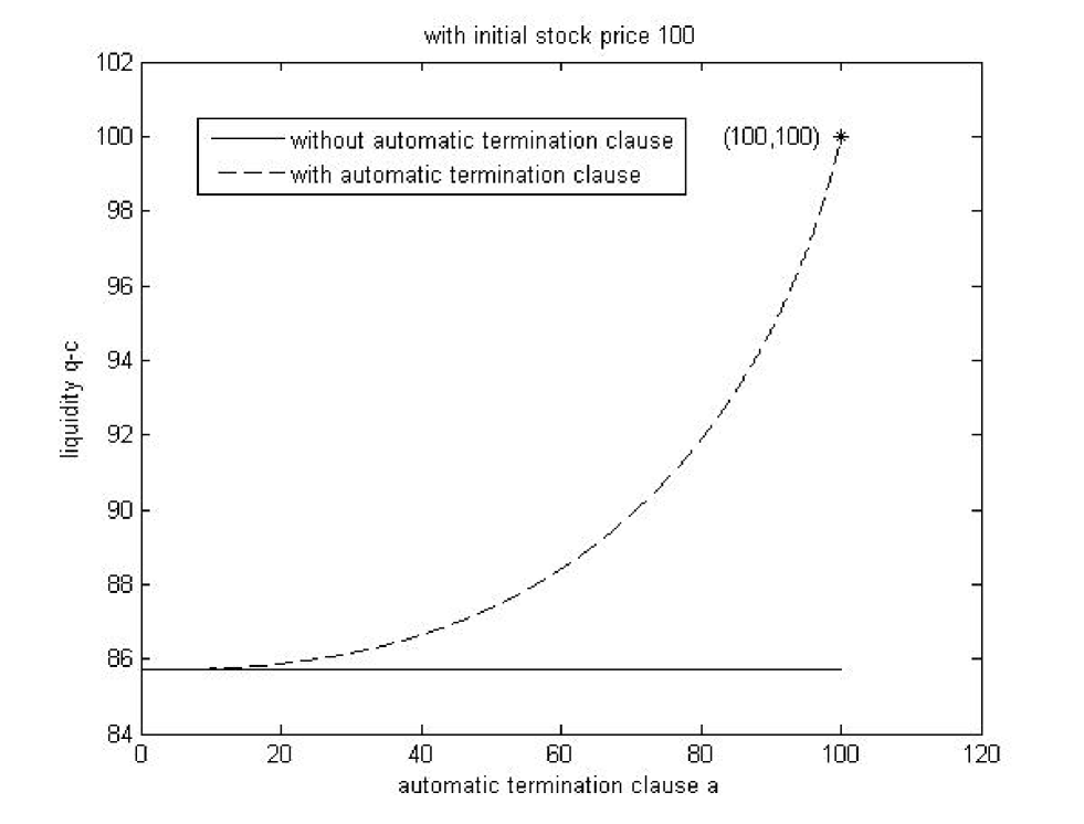
In this section we first consider a stock loan contract with an automatic termination clause $a$ ( $a\in[0,q]$ ), $r=0.05,\gamma=0.07,\sigma=0.15,\delta=0.01,q=100$ and $S_{0}=100$ . We will give six numerical examples to show that how the liquidity, optimal strategy $b(a)$ , initial value $f_{a}(x)$ and initial cash $q-c$ depend on automatic termination clause $a$ , respectively.

Example 7.1.

We see from graph1 below that the liquidity obtained with automatic termination clause is larger than the circumstance without the automatic termination clause. When the initial stock price $S_{0}=100$ and $a=100$ , the client just sell the stock to the bank by the stock loan contract with automatic termination clause.

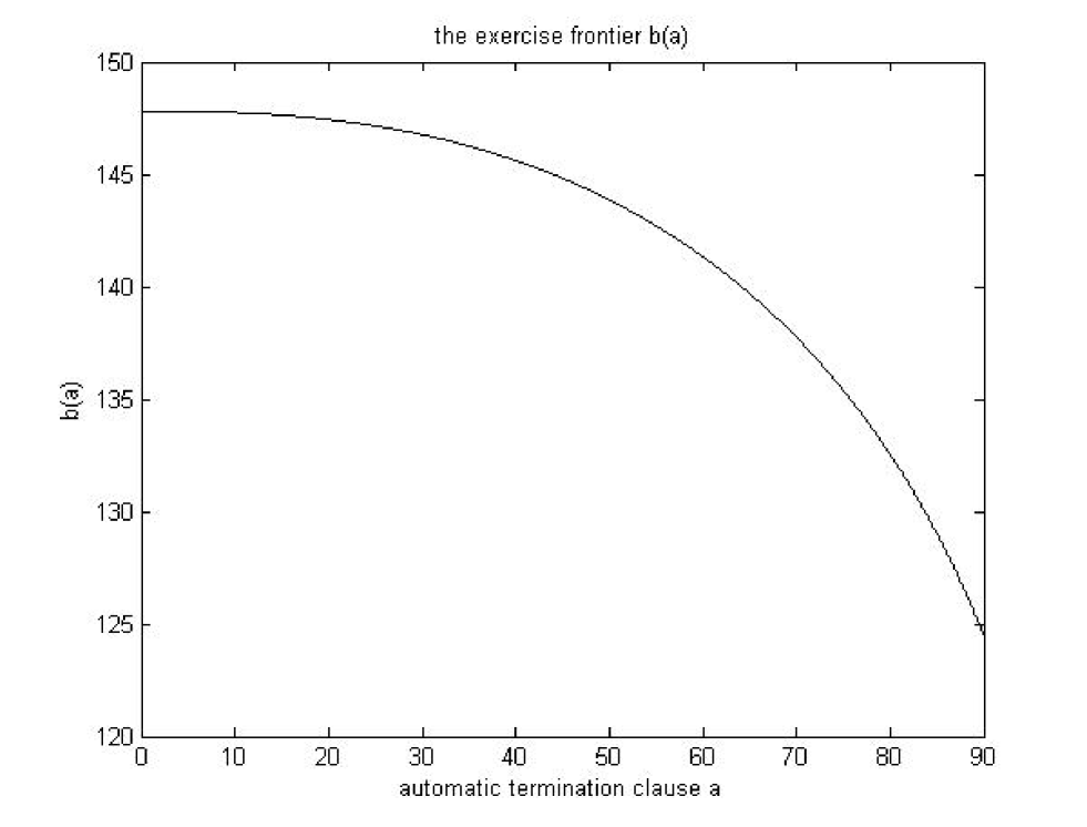
Refer to caption — Figure 1. $\gamma=0.07,r=0.05,\sigma=0.15,\delta=0.01,q=100,S_{0}=100$

Example 7.2.

We see from graph 5 below that $b$ is an function of $a$ . Both the client and the bank will take the deal when the initial stock price is in between $a$ and $b(a)$ . The client can determine the strategy with automatic termination clause $a$ . The exercise frontier $b(a)$ is decreasing with respect to $a$ .

Example 7.3.

The graph 3 below is a graph of initial value $f_{a}(x)$ of the stock loan with different automatic termination clause $(a=80,60,40,1)$ . We see from the graph that the initial value $f_{a}(x)$ is decreasing w.r.t. $a$ . Since $c=f(S_{0})-S_{0}+q$ , $c$ is also decreasing w.r.t. $a$ . This fact is consistent with the bank can reduce risk by introducing an automatic termination clause into the stock loan contract (see graph 1).

Example 7.4.

From graph 4 below we see that the initial cash $q-c$ is increasing with respect to initial stock price on $[a,b(a)]$ . When the initial stock price is less than $a$ , the client just sells the stock to the bank by the stock loan contract, the bank have no interest to do the business. In fact there is no transaction between the bank and the client.

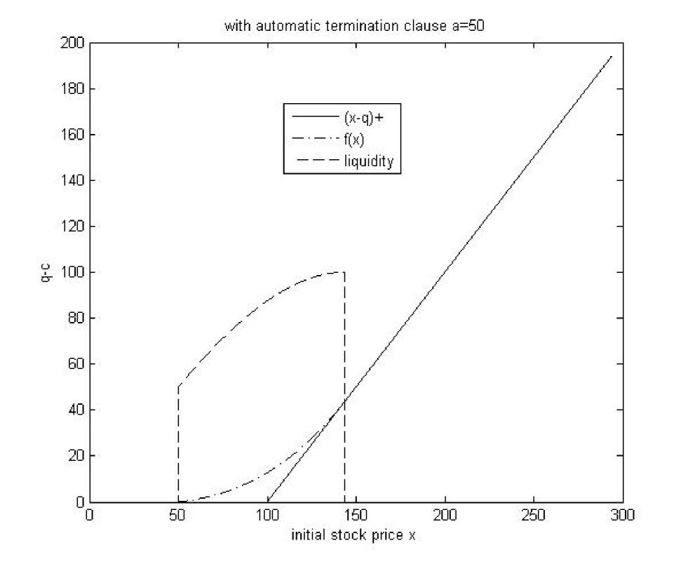
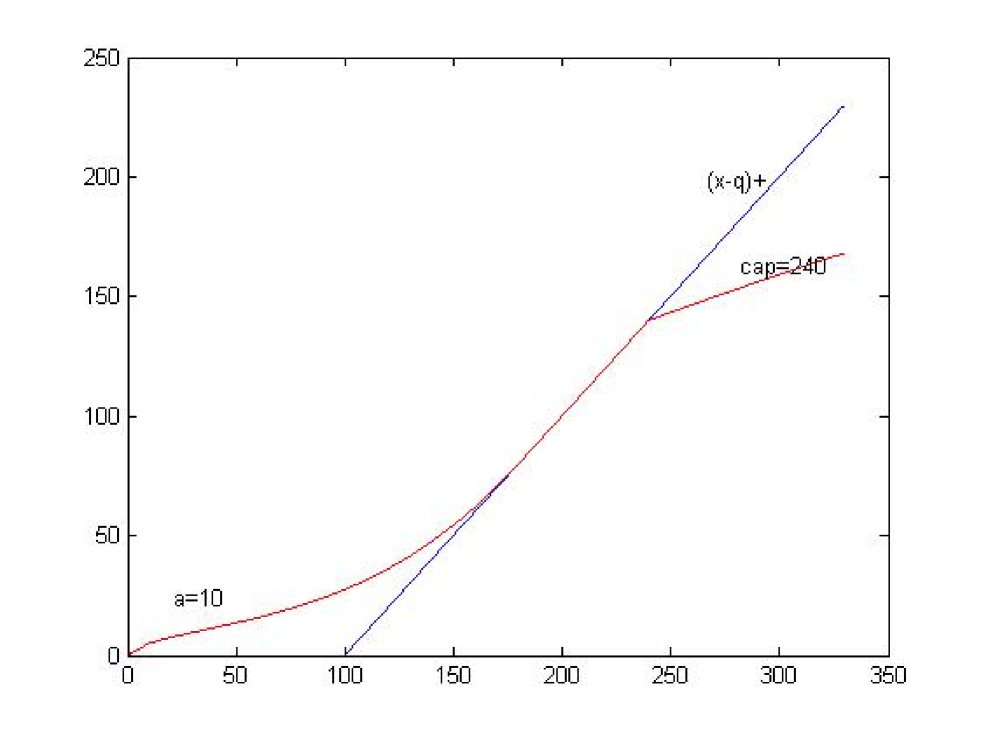
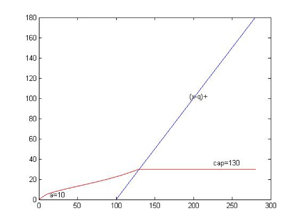
Then we consider a stock loan contract with automatic termination clause $a$ , cap $L$ and margin $k$ .

Example 7.5.

The graph 5 below shows that the function $b(a,k)$ . We see that for a given contract the client can choose the optimal excise time.

Example 7.6.

The graphs 6 and 7 below show that the function $f_{a}(x)$ . Comparison of the two graphs show the client can get more flexibility by lower cost.

8. Conclusion

In this paper, based on practical transactions between a bank and a client, we have established a mathematical model for stock loan with an automatic termination clause, cap and margin. The model can be considered a generalized perpetual American contingent claim with possibly negative interest rate. We have shown that variational inequality method can solve this kind of stock loans. Using the variational inequality method we have been able to derive explicitly the value of such a loan, ranges of fair values of other key parameters, relationships among the key parameters, and the optimal terminable exercise times. Moreover, we have checked that the clause $a$ , cap $L$ and margin $k$ are important factors in a stock loan contract by numerical results in examples 1-6.

9. Appendix

Lemma 9.1.

If $\delta>0$ and $\gamma-r+\delta\geq 0$ , then $\tilde{g}(y)$ is convex in the region $[\frac{q}{a},\infty)$ .

Proof.

It follows from proof of Proposition 4.1 that there exists $y^{*}$ in the region $(\frac{q}{a},\infty)$ such that $\tilde{g}(y^{*})=0$ . Noticing that

$\displaystyle\tilde{g}^{{}^{\prime\prime}}(y)$	$\displaystyle=$	$\displaystyle(\lambda_{1}-1)(\lambda_{1}+1-\lambda_{2})(\lambda_{1}-\lambda_{2})y^{\lambda_{1}-\lambda_{2}-1}$
		$\displaystyle-\frac{q}{a}\lambda_{1}(\lambda_{1}-\lambda_{2})(\lambda_{1}-\lambda_{2}-1)y^{\lambda_{1}-\lambda_{2}-2}$
	$\displaystyle=$	$\displaystyle(\lambda_{1}-\lambda_{2})\lambda_{1}(\lambda_{1}-1)y^{\lambda_{1}-2}h(y),\forall y\geq\frac{q}{a},$

where $h(y)$ is

\displaystyle h(y)=\frac{\lambda_{1}+1-\lambda_{2}}{\lambda_{1}}y^{1-\lambda_{2}}-\frac{q}{a}\frac{\lambda_{1}-1-\lambda_{2}}{\lambda_{1}-1}y^{-\lambda_{2}}\geq 0,\forall y\geq\frac{q}{a},

(9.1)

it suffices to show that $\tilde{g}^{{}^{\prime\prime}}(y)\geq 0,y\geq\frac{q}{a}$ for the uniqueness of $y^{*}$ . For this we only need to prove $h(y)\geq 0,\ \forall y\geq\frac{q}{a}$ . Since

\displaystyle h^{{}^{\prime}}(y)=\frac{\lambda_{1}+1-\lambda_{2}}{\lambda_{1}}(1-\lambda_{2})y^{-\lambda_{2}}+\frac{q}{a}\frac{\lambda_{1}-1-\lambda_{2}}{\lambda_{1}-1}\lambda_{2}y^{-\lambda_{2}-1},

we prove (9.1) in following three cases. Case of $\delta>0,\gamma>r$ . In this case we have $\lambda_{1}>1>\lambda_{2}>0$ . If $\lambda_{1}-\lambda_{2}\geq 1$ , then $h^{{}^{\prime}}(y)\geq 0,\ y\geq\frac{q}{a}$ . So

\displaystyle h(y)\geq h(\frac{q}{a})>0,y\geq\frac{q}{a}.

If $\lambda_{1}-\lambda_{2}<1$ , then

\displaystyle h(y)>\frac{\lambda_{1}+1-\lambda_{2}}{\lambda_{1}}y^{1-\lambda_{2}}\geq\frac{\lambda_{1}+1-\lambda_{2}}{\lambda_{1}}(\frac{q}{a})^{1-\lambda_{2}}>1,\ y\geq\frac{q}{a}.

Therefore (9.1) implies the convexity of $\tilde{g}(y)$ . Case of $\delta>0,\gamma=r$ . In this case we have $\lambda_{1}>1>\lambda_{2}=0$ and

\displaystyle h(y)=\frac{\lambda_{1}+1-\lambda_{2}}{\lambda_{1}}y^{1-\lambda_{2}}-\frac{q}{a}\frac{\lambda_{1}-1-\lambda_{2}}{\lambda_{1}-1}\geq h(\frac{q}{a})>0,\ y\geq\frac{q}{a}.

Obviously, the convexity of $\tilde{g}(y)$ holds. Case of $\delta>0,\gamma<r$ and $\gamma-r+\delta\geq 0$ . In this case we have $\lambda_{1}>1>0>\lambda_{2}$ and

	$\displaystyle h^{{}^{\prime}}(y)$	$\displaystyle=$	$\displaystyle\frac{\lambda_{1}+1-\lambda_{2}}{\lambda_{1}}(1-\lambda_{2})y^{-\lambda_{2}}+\frac{q}{a}\frac{\lambda_{1}-1-\lambda_{2}}{\lambda_{1}-1}\lambda_{2}y^{-\lambda_{2}-1}$		(9.2)
		$\displaystyle>$	$\displaystyle\frac{q}{a}y^{-\lambda_{2}-1}(1-\lambda_{2})(\frac{\lambda_{1}+1-\lambda_{2}}{\lambda_{1}}-\frac{\lambda_{1}-1-\lambda_{2}}{\lambda_{1}-1}),\ y\geq\frac{q}{a},$		(9.2)

where the last inequality follows from $\lambda_{1}>1>0>\lambda_{2}>-(1-\lambda_{2})$ .

Since $\gamma-r+\delta\geq 0$ , by (3.21) we have

\displaystyle\lambda_{1}+\lambda_{2}=2\frac{\gamma-r+\delta}{\sigma^{2}}+1\geq 1.

Because

\displaystyle\frac{\lambda_{1}+1-\lambda_{2}}{\lambda_{1}}-\frac{\lambda_{1}-1-\lambda_{2}}{\lambda_{1}-1}\geq 0,

by (9.2), $h^{{}^{\prime}}(y)\geq 0,\ y>\frac{q}{a}$ and

\displaystyle h(y)\geq h(\frac{q}{a})=(\frac{q}{a})^{-\lambda_{2}}(\frac{\lambda_{1}+1-\lambda_{2}}{\lambda_{1}}-\frac{\lambda_{1}-1-\lambda_{2}}{\lambda_{1}-1})\geq 0.

The convexity holds. Thus we complete the proof. ∎

Acknowledgements. We are very grateful to Professor Jianming Xia for his conversation with us and providing original paper of [37] for us. We also thank Professor Yongqing Xu for being informed us their work [18]. Special thanks also go to the participants of the seminar stochastic analysis and finance at Tsinghua University for their feedbacks and useful conversations. This work is supported by Projects 10771114 and 11071136 of NSFC, Project 20060003001 of SRFDP, and SRF for ROCS, SEM, and the Korea Foundation for Advanced Studies. We would like to thank the institutions for the generous financial support.

References

[1] Avrama,F., Chana, T., Usabel, M.,2002. On the valuation ofconstant barrier options under spectrally one-sided exponential Levy models and Carr s approximation for American puts. Stochastic Processes and their Applications 100, 75 - 107.
[2] Baldi, P., Caramellino, L., Iovino, G., 1998. Pricing general barrier options: a numerical approach using sharp large deviations. Mathematical Finance 9, 293-322.
[3] Bin Gao, Jing-zhi Huang, Marti Subrahmanyam,2000. The valuation of American barrier options using the decomposition technique, Journal of Economic Dynamics and Control, Vol.24, 1783-1827.
[4] Boyle, P.P., Lau, S.H., 1994. Bumping up against the barrier with the binomial method. Journal of Derivatives 1, 6-14.
[5] Boyle, P.P., Tian, Y.S., 1999. Pricing lookback and barrier options under the CEV process. Journal of Financial and Quantitative Analysis 34, 241-264.
[6] BOYARCHENKO, S., LEVENDORSKII, S., 2002. BARRIER OPTIONS AND TOUCH-AND-OUT OPTIONS UNDER REGULAR L VY PROCESSES OF EXPONENTIAL TYPE. The Annals of Applied Probability, Vol. 12, No. 4, 1261-1298.
[7] Borodin, A. N., Salminen, P., 2002. Handbook of Brownian Motion-Facts and Formulae. Probability and its Applications, Birkh $\ddot{a}$ user Verlag, Basel, 2nd edition.
[8] Broadie, M., and J. Detemple (1997) The valuation of American options on multiple assets, Mathematical Finance, 7:241-286.
[9] Cheuk,T.H.F. and T.C.F. Vorst (1997) Shout floors, Net Exposure, 2, Novermber issue.
[10] Dai, M., Y.K. Kwok and L.X. Wu (2004) Optimal shouting policies of options with strike reset rights, Mathematical Finance, 14(3):383-401.
[11] Dai, M., Xu Z.Q. (2010) Optimal Redeeming Strategy of Stock Loans with finite maturity, accepted for publication in Mathematical Finance.
[12] Dayanik, S., Karatzas, I., 2003. On the optimal stopping problems for one-dimensional diffusions. Stochastic Process. Appl, 107, no. 2, 173-212.
[13] Detemple, J., S. Feng, and W. Tian (2003) The valuation of American call options on the minimum of two dividend-paying assets, Ann. Appl. Probab., 13:953-983.
[14] Fusaia, A., Recchioni, M.C., 2007. Analysis of quadrature methods for pricing discrete barrier options. Journal of Economic Dynamics and Control 31, 826-860.
[15] Fusai, G., 2001. Applications of Laplace transform for evaluating occupation time options and other derivatives. Ph.D. Thesis, Warwick Business School, University of Warwick.
[16] Gao, B., Huang, J., Subrahmanyam, M., 2000. The valuation of American barrier options using the decomposition technique. Journal of Economic Dynamics and Control 24, 1783-1827.
[17] Gerber, H., and E. Shiu (1996) Martingale approach to pricing perpetual American options on two stocks, Mathematical Finance, 3:87-106.
[18] Guangying Liu and Yongqing Xu, Capped stock loan, Computers and Mathematics with applications. 59(2010)3548-3558.
[19] Hui, C.H., Lo, C.F., Yuen, P.H., 2000. Comment on pricing double barrier options using Laplace transforms. Finance and Stochastic 4, 105-107.
[20] Hull, J.C.Options, Futures, and Other Derivatives, 4th ed., Prentice- Hall, Upper Saddle River, NJ, 2000.
[21] Jiang, L. (2002) Analysis of pricing American options on the maximum (minimum) of two risky assets, Interfaces and Free Boundary, 4:27-46.
[22] Karatzas, I., Shreve,S. E., 1991. Brownian motion and stochastic calculus. Springer-Verlag, New York.
[23] Karatzas, I., Shreve,S. E., 1998. Methods of mathematical finance. Springer-Verlag, New York.
[24] Karatzas, I., Wang, H., 2000. A Barrier Option of American Type. Appl Math Optim42,259-279.
[25] Kifer,Y., 2000. Game Options. Finance and Stochastics, 4:443-463.
[26] Kudryavtsev, O.,Levendorski, S., 2009. Fast and accurate pricing of barrier options under L vy processes. Finance Stoch13,531-562.
[27] Kunitomo, N., Ikeda, M., 1992. Pricing options with curved boundaries. Mathematical Finance 2, 275-298.
[28] Kyprianou, A.E., 2004. Some calculations for Israeli options. Finance and Stochastics, 8:73-86.
[29] Liang, Zongxia and Wu,Weiming: Variational inequality method in stock loans, 2008, Preprint. arxiv:1105.1358.
[30] Mijatovi, A., 2010. Local time and the pricing of time-dependent barrier options. Finance Stoch 14,13-48.
[31] Øksendal, B. and Sulem A., 2005. Applied stochastic control of jump diffusions. Springer.
[32] Pelsser, A., 2000. Pricing double barrier options using Laplace transforms. Finance and Stochastics 4, 95-104.
[33] Rich, D.R., 1994. The mathematical foundations of barrier option pricing theory. Advances in Futures and Options Research 7, 267-371.
[34] Shiryaev,A.N., Kabanov,Y.M., Kramkov, D.O. and Melnikov, A.V., 1994. Towards the theory of options of both European and American types II. Theory Prob.Appl, 39,61-102.
[35] Sanfelici, S., 2004. Galerkin infinite element approximation for pricing barrier options and options with discontinuous payoff. Decisions in Economics and Finance, DEF27, 125-151.
[36] Windcliff, H., P.A. Forsyth, and K.R. Vetzal (2001) Valuation of segregated funds: shout options with maturity extensions, Insurance: Mathematics and Economics, 29:1-21.
[37] Xia, J.M., Zhou,X.Y., 2007. Stock loans. Mathematical Finance, Vol.17, No.2, 307-317.
[38] Zhang, Q., and X.Y. Zhou (2009), Valuation of stock loans with regime switching, SIAM Journal on Control and Optimization, 48(3):1229-1250.
[39] Zvan, R., Vetzal, K.R.,Forsyth, P.A., 2000. PDE methods for pricing barrier options, Journal of Economic Dynamics and Control 24, 1563-1590.