Stretching convex domains to capture
many lattice points
Abstract.
We consider an optimal stretching problem for strictly convex domains in that are symmetric with respect to each coordinate hyperplane, where stretching refers to transformation by a diagonal matrix of determinant . Specifically, we prove that the stretched convex domain which captures the most positive lattice points in the large volume limit is balanced: the -dimensional measures of the intersections of the domain with each coordinate hyperplane are equal. Our results extend those of Antunes & Freitas, van den Berg, Bucur & Gittins, Ariturk & Laugesen, van den Berg & Gittins, and Gittins & Larson. The approach is motivated by the Fourier analysis techniques used to prove the classical result for the Gauss circle problem.
Key words and phrases:
Lattice point counting, shape optimization, decay of Fourier transform2010 Mathematics Subject Classification:
42B10, 52C07 (primary) and 11H06, 35P15, 90C27 (secondary)1. Introduction
1.1. Introduction
In [1] Antunes & Freitas introduced a new type of lattice point problem; namely, among all ellipses that are symmetric about the coordinate axes and of fixed area, which captures the most positive lattice points? More precisely, for what is:
Determining for fixed is challenging, even computationally [1]; however, Antunes & Freitas were able to prove that
i.e., the ellipse which captures the most positive lattice points for large areas approaches a circle. Moreover, a rate of convergence of at least
This lattice point counting problem was originally motivated by a problem in high frequency shape optimization. Suppose that is an rectangular domain. Then the eigenvalues of the Dirichlet Laplacian are of the form
Thus, there is a bijection between the Dirichlet eigenvalues less than , and the positive lattice points in the ellipse . Hence, the statement can also be interpreted as the statement that the rectangle that minimizes the Dirichlet eigenvalues in the high frequency limit approaches the square.
1.2. Neumann eigenvalues
A dual result for eigenvalues of the Neumann Laplacian was established by van den Berg, Bucur & Gittins [17], where as before is an rectangular domain. The eigenvalues of are of the form
and hence, the Neumann eigenvalues less than are in bijection with the nonnegative lattice points in the ellipse . In terms of a lattice point problem, van den Berg, Bucur & Gittins proved that if
then . That is, the ellipse which captures the least nonnegative lattice points in the large area limit approaches the circle; equivalently, the rectangle which maximizes the Neumann eigenvalues in the high frequency limit approaches the square.
1.3. Higher dimensions
Subsequently, the result for Dirichlet eigenvalues was generalized to three dimensions by Gittins & van den Berg [18], and recently to -dimensions for both the Dirichlet and Neumann cases by Gittins & Larson [5]. Specifically, Gittins & Larson show that in the cuboid of unit measure which minimizes the Dirichlet eigenvalues in the high frequency limit approaches the cube, and similarly, that the cuboid of unit measure which maximizes the Neumann Laplacian eigenvalues in the high frequency limit approaches the cube. Both the Dirichlet and Neumann cases have corresponding lattice point problems analogous to the -dimensional case. The Dirichlet case corresponds to the following lattice point problem. Suppose is a positive diagonal matrix of determinant . For , let
Then the result of [5] implies that . Moreover, Gittins & Larson [5] show the following error estimate holds for dimensions :
and furthermore, they show a slightly improved error rate holds for by applying a result of Götze [6]. In this paper, we establish a similar rate of convergence for general convex domains. We note that the Neumann case in -dimensions has an analogous dual formulation to the -dimensional case, and similar error estimates were established in [5]. We remark that results concerning the optimization of eigenvalues of the Laplacian with perimeter constraints have also been considered [2, 4, 16]. In particular, Bucur & Freitas [4] proved that any sequence of minimizers of the Dirichlet eigenvalues with a perimeter constraint converges to the unit disk in the high frequency limit, and that among -sided polygons, any sequence of minimizers converges to the regular -sided polygon in the high frequency limit.
1.4. Convex and concave curves
Laugesen & Liu [10] and Ariturk & Laugesen [3] generalized the two dimensional case of the above lattice point counting problems to certain classes of convex and concave curves. In particular, their results imply that among -ellipses for the -ball captures the most positive lattice points. More generally, Laugesen & Liu and Ariturk & Laugesen show that the curves which capture the most positive integer lattice points in the large area limit are balanced: the distance from the origin to their points of intersection with the -axis and -axis are equal.
1.5. Right triangles
The results of [3, 10] exclude the case. In contrast to other values of , for the case (where -ellipses are right triangles) Ariturk & Laugesen and Laugesen & Liu conjectured that the optimal triangle
“does not approach a 45-45-90 degree triangle as . Instead one seems to get an infinite limit set of optimal triangles” (from [10]).
The author and Steinerberger [11] recently proved this conjecture and showed that the limit set is fractal of Minkowski dimension at most . Furthermore, all triangles which are optimal for infinitely many infinitely large areas have rational slopes, are contained in , and have as a unique accumulation point.
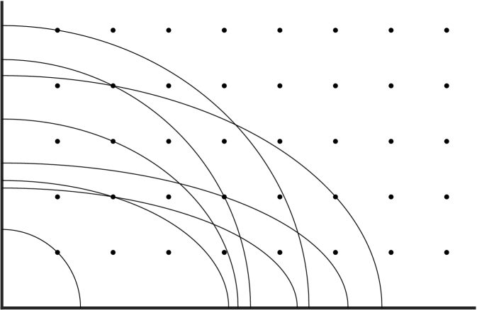
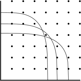
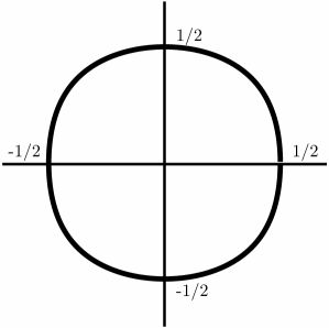
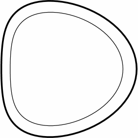
 |
 |
1.6. Relation to spectral asymptotics
Suppose that is a cuboid, and let denote the number of eigenvalues of the Dirichlet Laplacian that are less than
Then has a two-term asymptotic formula in terms of the volume and surface area of
where is the volume of the unit ball in . A similar asymptotic formula holds for the eigenvalues of the Neumann Laplacian , see [8]. We remark that in 1913, Weyl, see page 199 of [21], speculated about the existence of such a two-term asymptotic formula for more general domains in , and the problem of establishing the above two-term asymptotic formula for general domains became known as Weyl’s Conjecture, see [8]. In 1980, Ivrii [9] proved that this two-term asymptotic formula indeed holds for more general domains under certain conditions. Suppose that is an cuboid. Then the eigenvalues of the Dirichlet Laplacian are of the form
and thus, the eigenvalues of less than are in bijection with the positive lattice points in the ellipsoid . If this cuboid has unit measure , then its surface area is given by
Substituting into the above two-term asymptotic formula for for this cuboid gives
We emphasize that the error term in this asymptotic formula depends implicitly on the cuboid , and therefore, this asymptotic formula by itself is insufficient to determine which cuboid of unit measure maximizes as . Addressing this issue is the main challenge in [1, 5, 17, 18]. If we were to ignore the error term, then maximizing among cuboids of unit measure would be equivalent to minimizing . By the arithmetic mean geometric mean inequality
with equality if and only if . Since , this inequality can be interpreted as an isoperimetric inequality for cuboids: the surface area of a cuboid of unit measure is greater than or equal to the surface area of the unit cube with equality if and only if the cuboid is the unit cube. Ultimately, after the main challenge of dealing with the error term has been appropriately handled, this isoperimetric inequality for cuboids is the reason that the cube is asymptotically optimal in [1, 5, 17, 18]. In this paper, we consider a positive lattice point counting problem in more general domains; specifically, we study the number of positive lattice points in a fixed convex domain that has been scaled by and stretched by a linear transformation represented by a positive diagonal matrix of determinant . In this generalized setting, the term similarly arises, and we use Fourier analysis to develop lattice point counting results which lead to uniform error estimates for optimal stretching problems.
1.7. Motivation
In this paper, our motivation is twofold: first, the results of Laugesen & Liu and Ariturk & Laugesen show that the asymptotic balancing observed in lattice point problems for ellipses [1, 5, 17, 18] extends from ellipses to a more general class of convex and concave curves, at least in two dimensions, and second, the analysis of the case in [11] shows that the convergence breaks down when the curves become flat. This phenomenon is common in harmonic analysis, where the decay of the Fourier transform is dependent on non-vanishing curvature. To briefly review the relation of Fourier analysis to lattice point problems, suppose is a function on of compact support. Then the Poisson summation formula states that
where denotes the Fourier transform of
Suppose that is the indicator function for a domain . Then the indicator function for the scaled domain is , whose Fourier transform, by a change of variables is
Moreover, since , if the Poisson summation formula could be applied to , it would express the number of lattice points inside as plus the sum of over the nonzero lattice points. Unfortunately, the Fourier transforms of indicator functions do not decay rapidly enough for the Poisson summation formula to be applied (these functions lack sufficient smoothness). However, this issue can be resolved by smoothing the indicator function by convolution with a bump function, and useful estimates can be obtained. This approach can be used to establish the classical
result for the Gauss circle problem accredited to Sierpiński [12], van der Corput [19], and Voronoi [20], which was the first non-trivial step towards the conjectured result:
for all . Currently the best known result is due to Huxley [7]. The argument for the error term for the circle in can be generalized for convex domains whose boundary has nowhere vanishing Gauss curvature [13]. This generalization results in the following bound on the number of enclosed lattice points:
In this paper, we follow a similar approach to the proof of this result, but additionally handle the effects of stretching the domain. More specifically, given a strictly convex domain which is symmetric with respect to each coordinate hyperplane, we consider the positive lattice points contained in the domain , where is a positive diagonal matrix of determinant , and is a scaling factor.
In the following we compute an asymptotic expansion for which includes both the effects of the diagonal transformation and scaling factor ; we use this expansion to derive uniform error estimates for an optimal stretching problem. The resulting theorem extends the results of [1, 3, 5, 17, 18]. We note that we do not completely recover the results of [3, 10], since our approach can only represent curves which can be realized as the boundary of a convex domain whose boundary has nowhere vanishing Gauss curvature. However, there is some hope that the presented framework could be used to fully generalize the results of Laugesen & Liu [10] and Ariturk & Laugesen [3] by using more delicate bounds on the decay of the Fourier transform. Thus the presented approach may be useful for proving further generalizations.
2. Main Result
2.1. Main Result
Suppose that is a bounded convex domain whose boundary is and has nowhere vanishing Gauss curvature. Furthermore, suppose that is symmetric with respect to each coordinate hyperplane and balanced in the following sense.
Definition 2.1.
We say that a bounded convex domain is balanced if
where denotes the -dimensional Lebesgue measure.
Note that the balanced assumption does not restrict the domains for which the below Theorem applies. Rather, the assumption that is balanced is equivalent to choosing the unique balanced representative for , where is a positive diagonal matrix. Suppose that is a positive definite diagonal matrix of determinant . To reiterate, we define
for scaling factor . That is to say, is the domain scaled by and transformed by .
 |
 |
Theorem 2.1.
Suppose and are as described above. Then for and ,
where the implicit constant is independent of and . Moreover, if
then
where the implicit constant is independent of and .
In the following remark, we describe specifically how the implicit constants in Theorem 2.1 depend on , and provide conditions under which the expansion and convergence rate results in Theorem 2.1 hold uniformly over a family of domains.
Remark 2.1.
The implicit constants in Theorem 2.1 which depend on the domain can be chosen in terms of the following three quantities: a lower bound on the Gauss curvature of , an upper bound on the diameter of , and a lower bound on the inradius of . Therefore, the result of Theorem 2.1 holds uniformly over any family of admissible domains, which have uniform bounds for these three quantities. Indeed, constants depending on enter the proof of Theorem 2.1 from three sources. First, we use a constant such that ; since contains the origin it suffices to choose equal to the diameter of . Second, we use a constant from Lemma 3.1; by the proof of Lemma 3.1, this constant can be chosen as one divided by the inradius of . Third, we implicitly use a constant when using the bound in Lemma 3.3 for the decay of the Fourier transform of the indicator function for ; this implicit constant can be chosen in terms of a lower bound on the Gauss curvature of the domain, cf. [13].
When is a -dimensional ellipsoid, the Theorem implies the Dirichlet Laplacian results of Gittins & Larson [5]. Applying the Theorem for dimension recovers the original result of Antunes & Freitas [1] and agrees with the error estimate in [10]. Specifically, in dimension , the set of all positive diagonal matrices of determinant is the -parameter family for and the result of the Theorem can be stated as:
Corollary 2.1.
In the case , the Theorem gives
and
As a second Corollary we can establish dual results for the nonnegative lattice point problem, which corresponds to the Neumann Laplacian results of Gittins & Larson [5].
Corollary 2.2.
Suppose and satisfy the hypotheses of the Theorem, and additionally suppose for a fixed constant . Then
where the implicit constant is independent of and . Moreover, if
then
where the implicit constant is independent of and .
The assumption is needed for the expansion to hold, but not necessary for the convergence results as it serves to avoid the case where contains more than order lattice points on the coordinate hyperplanes which is clearly non-optimal for the . The proof of this Corollary follows from the arguments in Step 3.3 of the proof of Theorem 2.1.
2.2. Generalization
In the following we describe a generalization of Theorem 2.1. In particular, we remark how Theorem 2.1 can be generalized to domains which are not necessarily symmetric with respect to each coordinate hyperplane by considering the lattice points rather than the positive lattice points .
Remark 2.2.
Suppose that is a bounded convex domain whose boundary is and has nowhere vanishing Gauss curvature. Moreover, suppose is balanced in the sense of Definition 2.1, and contains the origin. Define . Let be a positive diagonal matrix of determinant . Then
where the implicit constant is independent of and . Moreover, if
then
where the implicit constant is independent of and . The proof of this statement is immediate from Step 3.3 of the proof of Theorem 2.1.
3. Proof of main result
3.1. Proof strategy
Before discussing the technical details, we describe the proof strategy. The proof is divided into five steps. First, we establish a new lattice point counting result which holds uniformly over a family of positive diagonal matrices with determinant . Specifically, we show that
when where is a fixed constant. The key observation in the proof of this expansion is that the classical Fourier analysis techniques used to study the Gauss circle problem can be applied if the indicator function of the domain is mollified by a bump function which has been appropriately stretched and scaled. Second, as a consequence of this result we show that the number of lattice points on the coordinate hyperplanes is, as expected, equal to plus an appropriate error term; specifically,
where denotes the intersection of with the hyperplane orthogonal to the -th coordinate vector. Third, we combine these two results to produce a positive lattice point counting result for :
Fourth, we show that this positive lattice point counting result implies that
where the is taken over positive diagonal matrices of determinant . We note that clearly since otherwise will not contain any positive lattice points; we proceed by considering two cases. First, we consider the case where
where our positive lattice point counting result for provides no information because the error term is order . However, in such an extreme situation we are able to independently show non-optimality. Second, we assume that
and use the positive lattice point counting result to show convergence. Specifically, we assume
Substituting into the positive lattice point counting result for gives
where is a fixed constant. Since the term in the parentheses we eventually be positive, and hence, comparison to the case where implies convergence. Fifth, and finally, given the fact that converges to we establish the convergence rate
using a standard arithmetic mean geometric mean argument.
3.2. Useful lemmata
The proof of the main result relies on three lemmata: two geometric in nature, and one related to the decay of the Fourier transform of indicator functions of convex domains with nowhere vanishing Gauss curvature. Lemmata 3.1 and 3.2 are proved in this section, and are motivated by similar technical results in [14], while Lemma 3.3 appears in standard references, cf., [13, 14, 15].
Lemma 3.1.
Suppose that is a bounded convex open domain which contains the origin. Then there exists a constant such that for all , all , and all
Proof.
Since is open, bounded, and contains the origin , there exists a constant such that
Set , and suppose that , , and are given. Then
and therefore,
where the final inclusion follows from the convexity of . ∎
The application of this Lemma to lattice point counting problems occurs when developing bounds for indicator functions in terms of mollified indicator functions. Specifically, Lemma 3.1 is typically applied as follows. Suppose is the indicator function for the set , and define
which is the indicator function for . Let denote a bump function supported on the unit ball which integrates to . Set
Suppose is chosen in accordance to Lemma 3.1. Then we claim that for all
where denotes convolution. Indeed, by the choice of , for all
Therefore, if , then
In the proof of the Theorem in the following section a similar result is required. However, in this case the indicator functions and bump functions under consideration are transformed by a positive diagonal linear transformation of determinant . More precisely, we consider
where is a positive diagonal matrix of determinant . Let
In the following Lemma, we repeat the above analysis to develop upper and lower bounds for in terms of the smoothed version .
Lemma 3.2.
Suppose and are as defined above. Then there exists a constant such that for all , all , and all positive diagonal matrices of determinant
for all .
Proof.
By Lemma 3.1 we may choose a constant such that for all and all
To establish the upper bound it suffices to show that . By definition
Since is a diagonal matrix of determinant , by a change of variables of integration we conclude
If , then by the choice of we have , when . Thus
which establishes the upper bound. Next, to establish the lower bound we show that . Let and . By Lemma 3.1
Writing the contrapositive of this statement in terms of and gives
Using the same change of variables of integration as above, we have
If , then the derived implication implies that for all ; thus
which completes the proof. ∎
Lemma 3.3.
Suppose is a bounded convex domain with boundary with nowhere vanishing Gauss curvature. If is the indicator function of , then
That is to say, the Fourier transform of an indicator function decays one order better than the Fourier transform of the corresponding surface carried measure , which decays like
The proof of this lemma involves an integration by parts of an expression for the Fourier transform of the corresponding surface carried measure, which is where the extra order of convergence arises.
3.3. Proof of Theorem 2.1
For clarity, we have divided the proof of the Theorem into five steps. First, we fix notation. We say
for a fixed constant only depending on . Throughout the proof, we assume that , , and that is a bounded convex domain with a boundary with nowhere vanishing Gauss curvature. In particular, we assume that
Let denote a positive diagonal matrix of determinant . Without loss of generality we may assume that , and set .
Step 3.1.
Suppose . Then
where the implicit constant is independent of and .
Proof.
Let denote the indicator function for the given domain , and set
where and for some bump function supported on the unit ball in and such that
We denote our “smoothed” approximation of the number of lattice points enclosed by by
Since is and of compact support, by the Poisson summation formula
Since and , we can break the sum up into three parts:
Since is the Fourier transform of an indicator function of a convex domain with nowhere vanishing Gauss curvature, it follows from Lemma 3.3 that
Furthermore, since is the Fourier transform of a function with compact support if follows that
for all . To evaluate the first sum we use the fact that , and
Therefore,
The sum on the right hand side can be compared to the integral
Thus we conclude that
For the second sum, we use the fact that
and use the same decay of as before. This yields
Hence
We can bound the sum on the right hand side by comparison to the integral
So
Moreover, since the bound for both sums is the same
Set
Substituting this value of into the last inequality yields
By Lemma 3.2 there exists a constant such that for all , all , and all positive diagonal matrices of determinant
for all . However, we do not in general know that . Therefore, in the following we consider two cases:
Case 1
If , then
Thus, we may apply Lemma 3.2 to conclude
Therefore, by the definition of
Moreover, since applying the bound derived above gives
and similarly,
Therefore, we conclude
Note can be fixed such that it only depends on (more specifically, dependent only on the dimension of ), so the proof is complete for this case.
Case 2
If , then we define
Since the determinant of is equal to , there exists such that
Define
Suppose . Then by construction
By the domain monotonicity of lattice point counting and the result from Case 1
Since and the constants and only depend on we conclude that
where the implicit constant only depends on . This completes the proof of Step 3.1.
∎
Step 3.2.
Suppose that , and assume that is balanced in the sense of Definition 2.1. Let denote the intersection of with the coordinate hyperplane orthogonal to the -th coordinate vector. Then
where the implicit constant is independent of and .
Proof.
If , then the statement is trivial. We consider two cases: and .
Case 1
If the dimension , then the set of positive diagonal matrices of determinant is the -parameter family . Therefore, it suffices to show that
for . In this case, and are the intersection of with the -axis and -axis, respectively. Moreover, since we have assumed is balanced for . Therefore, when is scaled by and transformed by , the total number of points on the axes will be , and thus the above statement holds.
Case 2
Suppose the dimension . Let denote the positive diagonal matrix formed by removing the -th row and -th column from . Write:
Observe that
Therefore, by the result from Step 3.1:
Observe that the total contribution of to the right hand side of this inequality is
Therefore, bounding by gives
A direct computation shows that
Thus, since we have assumed that , it follows that
Therefore, we obtain the bound
By the balanced assumption . Therefore, summing over yields
Next, we will use a similar argument to analyze , where and denotes the matrix formed by removing the -th and -th rows, and -th and -th columns from . Write:
In this case, applying Step 3.1 yields:
Observe that the total contribution of and to the right hand side is
Therefore, bounding by yields the bound
A direct computation yields:
Therefore, since we have assumed , it follows that
Similarly, it follows that
Therefore, we conclude that
Summing over gives
Recall that we previously established the inequality
These last two inequalities can be used to deduce the result in combination with the observation that:
and
∎
Step 3.3.
Assume that is balanced in the sense of Definition 2.1 and is symmetric with respect to each coordinate hyperplane. Then
Proof.
We partition the proof into two cases:
Case 1
Case 2
If , then we argue as follows. Recall that is a constant such that . Therefore, if , then and hence
In particular, it follows that
Therefore, the statement to prove reduces to
which trivially holds because the error term dominates the right hand side since . ∎
Step 3.4.
Suppose that is balanced in the sense of Definition 2.1 and is symmetric with respect to each coordinate hyperplane. Let
where the ranges over all positive diagonal matrices of determinant . Write . Without loss of generality suppose and let . Then
Remark 3.1.
Two technical remarks are in order about the definition of . First, we argue why the exists. As noted in Step 3.3, if , then will not contain any positive lattice points; therefore, the admissible for the can be restricted to those satisfying
where is a constant such that . Since the set contains finitely many positive lattice points, we conclude that the exists. Second, when the is not unique, should be interpreted as being equal to an arbitrary element from the maximal set; all convergence results are independent of this choice.
Proof of Step 3.4.
By the argument in Case 2 of Step 3.3, we may assume . First, we will suppose that there exists a constant such that
for arbitrarily large values . That is to say, we suppose that there exists a sequence tending towards infinity such that . We show that this assumption leads to a contradiction, which implies that
While producing this contradiction, we write and to simplify notation. Let denote the indicator function for . Then
Let , and let denote the matrix formed by removing the -st row and -st column from . With this notation
Since by assumption , and , we have
For simplicity, assume . In the course of the proof, we will only use the fact that is bounded above by a fixed constant. We remark that the method of estimating the sum in this part of the proof is similar to the arguments in [5, 18]. With the notation
We assert that:
Indeed, each lattice point can be identified with the -dimensional cube with sides parallel to the coordinates axes and vertices and , where denotes a -dimensional vector of ones. Since the set is convex, each of these cubes is contained in and their first coordinate is equal to . Moreover, this collection of cubes is disjoint since each pair of vertices is unique. Therefore, the sum is a lower approximation of the integral. Thus we have
Define the function by
The function is supported on some interval such that , where is a constant such that . Define
where denotes the -dimensional Lebesgue measure, and where the factor arises since the integral is taken over . Since and it follows that
Since is symmetric about the coordinate axes and is strictly convex, the maximum value of occurs at , is strictly decreasing on , and . Moreover, since we assume the boundary of is the function is certainly , which is sufficient for our purposes. Integrating on yields
However, our previous arguments show that
We assert that there exists such that
Indeed, the sum on the left hand side is a lower Riemann sum for the integral of the strictly decreasing function . Moreover, the constant can be chosen to hold uniformly for any lower Riemann sum of the integral which discretizes the integral into at most pieces.

Therefore, we conclude that
However, applying Step 3.3 with yields
When is sufficiently large
which contradicts the optimality of such . Therefore, we conclude that
By the Step 3.3 of the proof:
Substituting yields
for some constant . Since , we may choose large enough such that
Thus for large enough ,
However, if such a situation is optimal, it must be competitive with the situation , where
Therefore, we conclude that
which implies
Therefore, the set of optimal is uniformly bounded. Convergence then immediately follows from the result from Step 3.3, i.e., from the equation:
Indeed, since is uniformly bounded the second term determines the effect of when is large. Therefore, in order to maximize the coefficient of must be minimized. More precisely, can be characterized in terms of the following minimization problem
where the is taken over positive diagonal matrices of determinant such that , where is a fixed constant. By the arithmetic mean geometric mean inequality, any positive diagonal matrix of determinant satisfies
with equality if and only if . Therefore, we conclude that
Since is a continuous function, and equality holds in the arithmetic mean geometric mean inequality if and only if we conclude
as was to be shown. ∎
In the fifth step, we establish a rate of convergence.
Step 3.5.
Suppose that is balanced in the sense of Definition 2.1 and is symmetric with respect to each coordinate hyperplane. Let
where the ranges over all positive diagonal matrices of determinant . Then
Proof.
Applying the result of Step 3.3 for gives
By the arithmetic mean geometric mean inequality
Therefore, since maximizes over all , we must have
which simplifies to
To complete the proof it suffices to show that:
Indeed then,
Without loss of generality, suppose that
There are two cases to consider
Case 1
. In this case, suppose that where . Then
Since the determinant of is equal , it follows that the product . Therefore, by the arithmetic mean geometric mean inequality,
Expanding the left hand side in a Taylor series yields
And therefore, when is sufficiently small,
Case 2
. Suppose that . When is sufficiently small
Furthermore, since the determinant of is equal to
Therefore, by the arithmetic mean geometric mean inequality
Expanding the left hand side in a Taylor series yields
Therefore, when is sufficiently small,
Moreover, in either case
and the proof is complete. ∎
Acknowledgment. We are grateful to Stefan Steinerberger for many useful discussions, and Andrei Deneanu for insightful comments. Additionally, we would like to thank Richard Laugesen for valuable feedback leading to corrections in the proof and a much improved exposition, and the referees for their helpful comments.
References
- [1] P. R. S. Antunes and P. Freitas. Optimal spectral rectangles and lattice ellipses. Proc. Roy. Soc. London Ser. A, 469(2150), 2012.
- [2] P. R. S. Antunes and P. Freitas. Optimisation of eigenvalues of the Dirichlet Laplacian with a surface area restriction. Appl. Math. Optim., 73(2):313–328, 2016.
- [3] S. Ariturk and R. S. Laugesen. Optimal stretching for lattice points under convex curves. Port. Math., 74(2):91–114, 2017.
- [4] D. Bucur and P. Freitas. Asymptotic behaviour of optimal spectral planar domains with fixed perimeter. J. Math. Phys., 54(5):053504, 2013.
- [5] K. Gittins and S. Larson. Asymptotic behaviour of cuboids optimising Laplacian eigenvalues. S. Integr. Equ. Oper. Theory, 89(4):607–629, 2017.
- [6] F. Götze. Lattice point problems and values of quadratic forms. Invent. Math., 157:195-225, 2004.
- [7] M. N. Huxley. Exponential sums and lattice points III. Proc. London Math. Soc., 87:591, 2003.
- [8] V. Ivrii. 100 years of Weyl’s law. Bull. Math. Sci., 6(3):379–452, 2016.
- [9] V. Ivrii. On the second term of the spectral asymptotics for the Laplace-Beltrami operator on manifolds with boundary. Funktsional. Anal. i Prilozhen., 14(2):25–24, 1980.
- [10] R. Laugesen and S. Liu. Optimal stretching for lattice points and eigenvalues. ArXiv e-prints (to appear in Ark. Mat.), September 2016.
- [11] N. F. Marshall and S. Steinerberger. Triangles capturing many lattice points. ArXiv e-prints, June 2017.
- [12] W. Sierpiński. O pewnem zagadneniu w rachunku funkcyj asymptotznych. Prace Mat. Fiz, 17:77–118, 1906.
- [13] E. M. Stein. Harmonic Analysis: Real-Variable Methods, Orthogonality, and Oscillatory Integrals. Princeton University Press, Princeton, New Jersey, 1993.
- [14] E. M. Stein and Rami Shakarchi. Princeton Lectures in Analysis: Functional Analysis, Princeton University Press, Princeton, New Jersey, 2011.
- [15] G. Travaglini. Average Decay of the Fourier Transform. In L. Brandolini, L. Colzani, A. Iosevich, G. Travaglini, editors. Fourier Analysis and Convexity, pages 245–268, Birkhäuser, 2004.
- [16] M. van den Berg. On the minimization of Dirichlet eigenvalues. Bull. Lond. Math. Soc., 47(1):143–155, 2015.
- [17] M. van den Berg, D. Bucur, and K. Gittins. Maximising Neumann eigenvalues on rectangles. Bull. Lond. Math. Soc., 48(5):877–894, 2016.
- [18] M. van den Berg and K. Gittins. Minimising Dirichlet eigenvalues on cuboids of unit measure. Mathematika, 63:469–482, 2017.
- [19] J. G. van der Corput. Neue zahlentheoretische Abschätzungen. Math. Ann., 89:215–254, 1923.
- [20] G. Voronoi. Sur un problème du calcul des fonctions asymptotiques. J. Reine Angew. Math., 126:241–282, 1903.
- [21] H. Weyl. Über die Randwertaufgabe der Strahlungstheorie und asymptotische Spektralgesetze. J. Reine Angew. Math., 143(3):177–202, 1913.