Strictly Anomaly Mediated Supersymmetry Breaking
Abstract:
We consider an extension of the MSSM with anomaly mediation as the only source of supersymmetry-breaking, and the tachyonic slepton problem solved by a gauged U(1) symmetry. The extra gauge symmetry is broken at high energies in a manner preserving supersymmetry, while also introducing both the see-saw mechanism for neutrino masses, and the Higgs -term. We call the model sAMSB (strictly anomaly mediated supersymmetry breaking.
We present typical spectra for the model and compare them with those from so-called minimal anomaly mediated supersymmetry breaking. We find a SM-like Higgs of mass 125 GeV with a gravitino mass of 140 TeV and . However, the muon anomalous magnetic moment is 3 away from the experimental value.
The model naturally produces a period of hybrid inflation, which can exit to a false vacuum characterised by large Higgs vevs, reaching the true ground state after a period of thermal inflation. The scalar spectral index is reduced to approximately 0.975, and the correct abundance of neutralino dark matter can be produced by decays of thermally-produced gravitinos, provided the gravitino mass (and hence the Higgs mass) is high. Naturally light cosmic strings are produced, satisfying bounds from the Cosmic Microwave Background. The complementary pulsar timing and cosmic ray bounds require that strings decay primarily via loops into gravitational waves. Unless the loops are extremely small, the next generation pulsar timing array will rule out or detect the string-derived gravitational radiation background in this model.
1 Introduction
The SM Higgs-like particle of mass recently discovered at the LHC [1, 2] strongly constrains future model building, while recent negative results from both the Tevatron and LHC in searches for sparticles place increasing pressure on models with low energy supersymmetry. Here we explore a specific supersymmetric model in which the low energy spectrum is that of the Minimal Supersymmetric Standard Model (MSSM), but the gauge symmetry is augmented by an extra gauged U(1) symmetry, , spontaneously broken at high energies in a manner which affects both physics at the supersymmetry breaking scale and physics at high scales characterising inflation and cosmic strings.
The broad features of the model are independent of the source of supersymmetry breaking, but if we assume that this source is in fact anomaly mediation (AMSB) [3]-[5], then there arises an interesting interplay between the low energy physics (and in particular the Higgs -term) and the high energy physics involving strings and inflation. Moreover the breaking of solves the tachyonic slepton problem characteristic of AMSB [5, 6].
We first presented this specific model in [7], in a form where we also introduced a Fayet-Iliopoulos (FI) term for the . Here we concentrate on the minimal formulation when there is no such term111Aside from the fact that this makes the model more appealing by removing an independent mass scale, we also thereby avoid confrontation with the conclusion of Komargodski and Seiberg [8] that a global theory with a FI term cannot be consistently embedded in supergravity. The model implements a form of AMSB which we refer to as strictly anomaly-mediated supersymmetry-breaking (sAMSB), by which we mean that there are no other sources of supersymmetry breaking beside the F-term of the conformal compensator field. As a consequence the soft parameters have an elegant renormalisation group (RG) invariant form. It therefore differs from so-called minimal AMSB(mAMSB), which posits an extra source of supersymmetry-breaking, instead of extra fields, in order to solve the tachyonic slepton problem. Our model is not quite a complete sAMSB implementation, in that it requires an extension to determine the soft parameter associated with the Higgs -term.
We begin by describing the symmetries and field content of the model and explaining in detail how the spontaneous breakdown of the symmetry at a large scale not only solves the AMSB tachyonic slepton problem, but also generates a Higgs term and the see-saw mechanism for neutrino masses. This outcome is achieved by the introduction of three new chiral superfields; , which is a gauge singlet and a pair of singlet fields which are oppositely charged under . We then exhibit characteristic sparticle spectra for the model; the calculations involved to obtain these are essentially as described in Refs. [9, 10], but allowing for a larger gravitino mass. We also discuss the fine-tuning issue raised by this, and compare the results of our model with results from the most popular (but, we will argue, less elegant) version of AMSB, generally called mAMSB. We will see that sAMSB generally keeps sleptons lighter than in mAMSB, which means that the contribution to the muon anomalous magnetic moment is typically higher for a given Higgs mass.
The theory incorporates a natural mechanism for supersymmetric F-term inflation, with the scalar component of as the inflaton. Previously, we concentrated on a region of parameter space such that inflation ended with a transition to a state with only the broken. There is, however, an interesting alternative that inflation ends with the development of vevs for the Higgs multiplets, , breaking the electroweak symmetry. A combination of the Higgs fields and the scalar components of the singlet fields is a flat direction, lifted by soft supersymmetry-breaking terms, and the normal low energy electroweak vacuum is achieved after a later period of thermal inflation. Approximately 17 e-foldings of thermal inflation reduce the number of e-foldings of high scale inflation, and therefore reduce the spectral index of scalar Cosmic Microwave Background (CMB) fluctuations to about 0.975. This is within about of the WMAP7 value.
The reheat temperature after this period of thermal inflation is around GeV, which means that there is no gravitino problem: gravitinos are very massive, more than 40 TeV, and so decay early enough not to be in conflict with nucleosynthesis. Indeed, the gravitino problem can turn into the gravitino solution for the typical AMSB feature of too low a dark matter density generated at freeze-out: the lightest supersymmetric particle (LSP) is mostly wino and has a relatively high annihilation cross-section. In our model a critical density of LSPs can be generated by gravitino decays, if the gravitino (and hence the LSP) is heavy enough.
The model also has the possibility of baryogenesis via leptogenesis following thermal inflation, with CP violation supplied by the neutrino sector. The field giving mass to right-handed neutrinos has an inflation-scale ( GeV) vacuum expectation value (vev), but if the lightest right-handed neutrino is sufficiently light to be generated at reheating after thermal inflation, a lepton asymmetry can be generated by its out-of-equilibrium decay.
There is a broken U(1) symmetry in the model, and cosmic strings with a GeV mass scale are formed, although not until the end of thermal inflation. There is a large Higgs condensate in the core of the string which spreads the string out to a width of order the supersymmetry-breaking scale, and reduces its mass per unit length by well over an order of magnitude. The strings satisfy CMB constraints on the mass per unit length from combined WMAP7 and small-scale observations. Their decays are constrained by pulsar timing observations in the case of gravitational waves and the diffuse -ray background in the case of particle production: the latter means that less than about 0.1% of the energy of the strings should end up as particles, and the former puts constraints on the average size of the loops at formation.
The model has the same field content as the hybrid inflation model [11, 12], but different charge assignments and couplings. hybrid inflation also has a singlet which is a natural inflaton candidate, but differs in other ways: for example, right-handed neutrinos have electroweak-scale masses, and the gravitino problem is countered by entropy generation.
The model also has the same field content as the BL model of Refs. [13], although as explained in section 3, the U(1)′ symmetry cannot be U(1)B-L in AMSB. It is also closely related to the model of Ref. [14], in which the fields , are SU(2)R triplets. This also has a flat direction involving the Higgs, although the authors did not pursue its consequences.
To summarise our results: at , sAMSB can accommodate a Higgs mass above 120 GeV for gravitino masses over 80 TeV, while accounting for the discrepancy in between the Standard Model (SM) theory and experiment to within would have favoured 80 TeV or lower. Larger values of allow a more massive Higgs: for we find a Higgs mass of 125 GeV for a gravitino mass of 140 TeV.
sAMSB also allows for an observationally consistent dark matter density, if the gravitino mass is over about 100 TeV, with the dark matter deriving from the decay of gravitinos produced from reheating after thermal inflation. The spectral index of scalar cosmological perturbations is within 1 of the WMAP7 value, and the observational bounds on cosmic strings can be satisfied if the strings decay into gravitational radiation. The model has also has a natural mechanism for baryogenesis via leptogenesis through the decays of right-handed neutrinos.
2 The AMSB soft terms
We will assume that supersymmetry breaking arises via the renormalisation group invariant form characteristic of Anomaly Mediation, so that the soft parameters for the gaugino mass , the interaction and the and mass terms and in the MSSM take the generic RG invariant form
| (1) | |||||
| (2) | |||||
| (3) | |||||
| (4) |
Here is the renormalisation scale, and is the gravitino mass; are the gauge -functions and is the chiral supermultiplet anomalous dimension matrix. are the Yukawa matrices, and is the superpotential Higgs -term. We will see that in our low energy theory, Eq. (3) is replaced, in fact, by
| (5) |
where the are charges corresponding to a U(1) symmetry. This term corresponds in form to the contribution of an FI D-term, and can be employed to obviate the tachyonic scalar problem characteristic of AMSB. How such a term can be generated (with AMSB) was first discussed in Ref. [5], and first applied to the MSSM in Ref. [6]. The basic idea was pursed in a number of papers [15]-[19]. For example, Ref. [15] demonstrated explicitly the UV insensitivity of the result, and Ref. [16] emphasised that the tachyonic problem could be solved using a single U(1) rather than a linear combination of two, the approach followed in Ref. [6]. An extension of the MSSM such that the spontaneous breaking of a gauged with an FI term gave rise to the term was written down in Ref. [9]. In [7] we developed an improved version of this model, retaining the possibility of a primordial FI term for ; here we will dispense with the FI term, and emphasise that we can nevertheless generate the term naturally with of , by breaking a symmetry at a large scale, without introducing an explicit FI term.
At first sight Eq. (5) resembles the formula for the scalar masses employed in the so-called mAMSB model, where the term is replaced by a universal scalar mass contribution . The differences are as follows:
-
•
The mAMSB involves the introduction of an additional source of supersymmetry breaking independent of the gravitino mass, while, as we shall see, Eq. (5) does not.
-
•
The parameter in Eq. (5) turns out to be more constrained than . This is associated with the fact that inevitably all the cannot have the same sign.
- •
It is these observations that prompts us to refer to our model as sAMSB. Note that, of course, we cannot “promote” the mAMSB into the sAMSB by the addition of additional heavier fields which cancel the associated anomaly; with an unbroken , any massive chiral multiplets will obviously make no contribution to this anomaly.
Eq. (4) is the most general form for that is consistent with RG invariance, as first remarked explicitly in Ref. [9]; the parameter is an arbitrary constant. For discussion of possible origins of from the underlying superconformal calculus formulation of supergravity see Refs. [5, 18, 19]. We will simply assume that the model can be generalised to produce such a term; the procedure which has, in fact, been generally followed. The presence of means that in sparticle spectrum calculations one is free to calculate (and the value of the Higgs -term, ) by minimising the Higgs potential at the electroweak scale in the usual way. (For , which is the value suggested by a straightforward use of the conformal compensator field [5], one might have hoped to use the minimisation conditions to determine , but it turns out this leads to a very small value of incompatible with gauge unification, because of the correspondingly large top Yukawa coupling [17]). We will see, however, that in our model the result for has implications for other parameters in the underlying theory which are constrained by cosmological considerations.
3 The symmetry
The MSSM (including right-handed neutrinos) admits two independent generation-blind anomaly-free U(1) symmetries. The possible charge assignments are shown in Table 1.
The SM gauged is ; this U(1) is of course anomaly free even in the absence of . is ; in the absence of this would have and U(1)-gravitational anomalies, but no mixed anomalies with the SM gauge group.
Our model will have, in addition, a pair of MSSM singlet fields with charges and a gauge singlet . In order to solve the tachyon slepton problem we will need that, for our new gauge symmetry , the charges have the same sign at low energies. As explained in Ref. [10], however, it is in fact more appropriate to input parameters at high energies, when in fact although necessarily , the range of acceptable values of includes negative ones; not negative enough, however, to allow to be .
Thus sAMSB has three input parameters , , , associated with the supersymmetry breaking sector, while mAMSB only has two: , . However, it turns out that because the allowed region is so restricted, sAMSB is the more predictive of the two. We will see this explicitly in section 6.
4 The superpotential and spontaneous breaking
The complete superpotential for our model is:
| (6) |
where is the MSSM superpotential, omitting the Higgs -term, and augmented by Yukawa couplings for the right-handed neutrinos, :
| (7) |
and
| (8) |
where are real and positive and is a symmetric matrix. The sign of the term above is chosen because with our conventions, in the electroweak vacuum where
| (9) |
we have .
The symmetry forbids the renormalisable and violating superpotential interaction terms of the form , , , , , and , as well as the mass terms , and and the linear term . Moreover contains the only cubic term involving that is allowed. Our superpotential Eq. (6) is completely natural, in the sense that it is invariant under a global -symmetry, with superfield charges
| (10) |
which forbids the remaining gauge invariant renormalisable terms (, , and ). This -symmetry also forbids the quartic superpotential terms and , which are allowed by the symmetry, and give rise to dimension 5 operators capable of causing proton decay [20]-[22]. It is easy to see, in fact, that the charges in Eq. (10) disallow B-violating operators in the superpotential of arbitrary dimension. Of course this -symmetry is broken by the soft supersymmetry breaking.
5 The Higgs potential
In this section we discuss the spontaneous breaking of the symmetry and its consequences. We shall assume is much larger than the scale of supersymmetry-breaking. (Such a large tadpole term has been disfavoured in the past; moreover it has been argued that it would generally be expected to lead to a large vev , but as we shall see this does not happen in our model.) It is then clear from the form of the superpotential as given in Eq. (8) that for an extremum that is supersymmetric (when we neglect supersymmetry-breaking) we will require non-zero vevs for and/or (in order to obtain ). The existence of competing vacua of this nature was noted in by Dvali et al in Ref. [14]; their model differs from ours in choice of gauge group (they have ) and supersymmetry-breaking mechanism.
Let us consider these two possibilities in turn.
5.1 The extremum
Retaining for the moment only the scalar fields (the scalar component of their upper case counterpart superfields) we write the scalar potential:
| (11) | |||||
Here, as well as soft terms dictated by Eqs. (2),(3), we also introduce a soft breaking term linear in . (In fact, according to Ref. [23], for a nonvanishing RG invariant form of we would require a quadratic term in in the superpotential, which in fact we do not have. We nevertheless consider the possible impact of a term, but will presently assume it is small, even if non-zero).
The potential depends on two explicit mass parameters, the gravitino mass and . Let us establish its minimum. Writing , and , we find
| (12) | |||||
| (13) | |||||
| (14) |
It follows easily from Eqs. (12),(13) that
| (15) | |||||
| (16) |
We now assume that . It is immediately clear from Eqs. (15),(16) that
| (17) |
and then from Eq. (14) that is . We thus obtain from Eq. (16) that
| (18) |
and from Eq. (14) that
| (19) |
Now the term is determined in accordance with Eq. (2):
| (20) |
denoting the charge by .
If we assume that then we find
| (21) |
For simplicity we shall assume that , so that the contributions to Eq. (19) and Eq. (21) are negligible.
Substituting back from Eqs. (17),(19) into Eq. (11), we obtain to leading order
| (22) |
Presently we shall compare this result with the analagous one associated with the extremum.
Supposing, however, that the extremum is indeed the relevant one, we obtain the Higgs -term
| (23) |
One might think that since is naturally determined above to be associated with the susy breaking scale (rather than the breaking scale) it would be necessary to minimise the whole Higgs potential (including ) in order to determine it. But if we retain, for example, the term in Eq. (14), the resulting correction to Eq. (19) is easily seen to be . Similarly, the Higgs vevs responsible for electroweak symmetry breaking do not affect Eqs. (19),(23) to an appreciable extent.
In Ref. [7], we naively estimated , concluding that would be at most rather than . The improved formula Eq. (23) changes this conclusion.
If we neglect terms of , it is easy to see from Eqs. (15),(16) that the breaking of preserves supersymmetry (since in this limit the two equations correspond to vanishing of the F-term and the D-term respectively); thus the gauge boson, its gaugino (with one combination of ) and the Higgs boson form a massive supermultiplet with mass , while the remaining combination of and and the other combination of form a massive chiral supermultiplet, with mass .
For large , all trace of the in the effective low energy Lagrangian disappears, except for contributions to the masses of the matter fields, arising from the D-term, which are naturally of the same order as the AMSB ones. Evidently also gets a large supersymmetric mass, as does the triplet, thus naturally implementing the see-saw mechanism. The generation of an appropriate -term via the vev of a singlet is reminiscent of the NMSSM (for a review of and references for the NMSSM see Ref. [24]). We stress, however, that our model differs in a crucial way from the NMSSM, in that the low energy spectrum is precisely that of the MSSM.
It is easy to show by substituting Eq. (18) back into the potential, Eq. (11) that the contribution to the slepton masses arising from the term which resolves the tachyonic slepton problem is given by
| (24) |
with corresponding contributions for the other scalar MSSM fields proportional to their charges. Now
| (25) |
where (at one loop)
| (26) |
and we have for simplicity taken to be diagonal.
Let us consider what sort of values of we require. In this context it is interesting to compare Fig. 1 of Ref. [9] with Fig. 1 of Ref. [10]. In both references, correspond to our respectively. In the former case the scalar masses are calculated at low energies, whereas in the latter they are calculated at gauge unification and then run down to the electroweak scale. This is why the allowed regions are different in the two cases. Since we are assuming is large, it is clear that the latter are more relevant to our situation. From Fig. 1 of Ref. [10] we see that suitable values would be
| (27) |
Notice that must necessarily be positive.
So, if we assume that the one-loop is dominated by its gauge contribution, consistent with our previous assumption that , we obtain
| (28) |
Now , so we see that it is easy to obtain the correct sign for .
For , we find
| (29) |
or
| (30) |
Of course with , we have ; but as describe earlier, it was shown in Ref. [10] that acceptable slepton masses nevertheless result when we run down to low energies. Clearly there are similar contributions to the masses of the other matter fields similar to Eq. (28), thus for example
| (31) |
In the notation of Ref. [10], Eq. (28), for example, is simply replaced by and with replacing , and all results presented for .
We emphasise once again the contrast between our model and conventional versions of the NMSSM, which does not, in basic form, contain an extra gauged U(1), but where a vev (of the scale of supersymmetry breaking) for the gauge singlet generates a Higgs -term in much the same way, as is done here. However, while in the NMSSM case the fields are very much part of the Higgs spectrum, here, in spite of the comparatively small -vev, the -quanta obtain large supersymmetric masses and are decoupled from the low energy physics, which becomes simply that of the MSSM. Another nice feature is the natural emergence of the see-saw mechanism via the spontaneous breaking of the . Evidently it will be feasible to associate the breaking scale given by Eq. (17) with the scale of gauge unification.
Although, as indicated above, we will be regarding as source of significant physics, it is worth briefly considering the limit . In that limit, the theory becomes simply the MSSM (including the Higgs -term) with the soft breaking terms given in Eq. (1)-Eq. (3) including the additional term, which resolves the tachyon problem. The explicit form of the terms proportional to the gravitino mass in these equations is easily derived using the conformal compensator field as described in Ref. [5]. Of course, although the resulting term in Eq. (3) has the form of an FI term, in the effective theory (for ) is not gauged and so we do not fall foul of the strictures of Ref. [8]. The conformal compensator field does not provide us with a straightforward derivation of Eq. (4); as described earlier, we will, like most previous authors, rely on the electroweak minimisation process to determine the Higgs -term.
5.2 The extremum
.
We now consider the scalar potential
| (32) | |||||
In Eq. (32) we have written the gauge coupling as , although its normalisation corresponds to the usual SM convention, not that appropriate for SU(5) unification. This is to avoid confusion with the coupling, .
We see that the potential is very similar to Eq. (11), the main difference being the presence of SU(2) and D-terms. To leading order in , only the SU(2) D-term depends on the relative direction in SU(2)-space of the two doublets; it follows that we can choose without loss of generality to set and , as in electroweak breaking, in order to obtain zero for the SU(2) D-term for . Minimisation of the potential then proceeds in a similar way to the previous section (with the replacement ) leading to
| (33) |
at the extremum. Here
| (34) | |||||
Let us compare the result for with that obtained for , in the previous section, Eq. (22). If we assume that the terms dominate throughout we obtain simply
| (35) |
and
| (36) |
where we have written the one loop -function as
| (37) |
and
| (38) | |||||
The coefficient is in general large, and larger than both and , so the condition for the extremum to have a lower energy than the one may be written
| (39) |
Alternatively, for the specific choice , which we will see in the next section leads to an acceptable electro-weak vacuum, we find that the same condition becomes
| (40) |
6 The sparticle spectrum
In this section we calculate sparticle spectra for the sAMSB model, and compare the results with typical mAMSB spectra. We shall be interested in seeking regions of parameter space with a “high” Higgs mass - that is, close to about 125 GeV as suggested by recent LHC data [1, 2] - and a supersymmetric contribution to the muon anomalous magnetic moment compatible with the experimental deviation from the Standard Model prediction, [25]. We will also wish to remain consistent with the negative results of recent LHC supersymmetry searches, see for example Refs. [26, 27].
We use the methodology of Ref. [10], which, as explained in Section 2, can also be applied to mAMSB by replacing the characteristic FI-type terms of sAMSB by a universal mass term .
We begin by choosing input values for , , , and at the gauge unification scale . Then we calculate the appropriate dimensionless coupling input values at the scale by an iterative procedure involving the sparticle spectrum, and the loop corrections to , , and , as described in Ref. [28]. We define gauge unification by the meeting point of and ; this scale, of around , we assume to be equal or close to the scale of breaking. For the top quark pole mass we use . All calculations are done in the approximation that we retain only third generation Yukawa couplings, ; thus the squarks and sleptons of the second generation are degenerate with the corresponding ones of the first generation.
We then determine a given sparticle pole mass by running the dimensionless couplings up to a certain scale chosen (by iteration) to be equal to the pole mass itself, and then implementing full one-loop corrections from Ref. [28], and two-loop corrections to the top quark mass [29]. We use two-loop anomalous dimensions and -functions throughout.
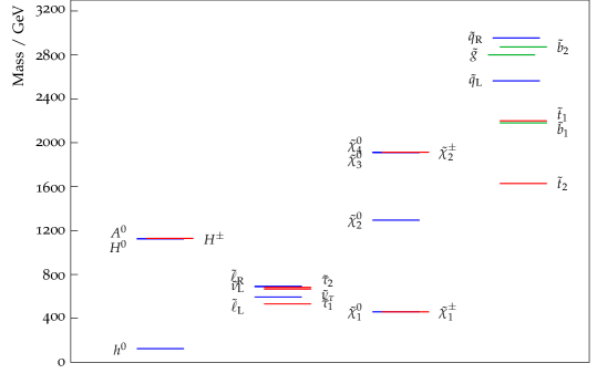
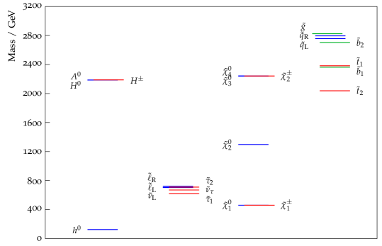
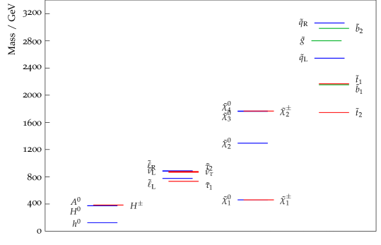
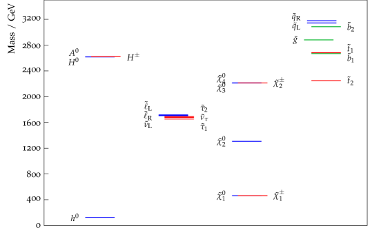
6.1 Mass spectra in sAMSB
We display some examples of spectra in Tables 2-5. In each Table, the columns are for different gravitino masses, all with with increasing with increasing gravitino mass so as to remain within the allowed region; obviously scales like from Eq. (28). (As already indicated, we input at , so the allowed region corresponds to that in Ref. [10] rather than that in Ref. [9] ). In Tables 2,4 the values are in the centre of the allowed region (at least for smaller values of ), whereas in Tables 3,5 is smaller so that lighter sleptons result. We see that varies little with ; for example in Table 2 changing from at to at . We thus find from Eq. (23) that
| (41) |
in order for the electro-weak vacuum to exist. We shall return to this formula when we have discussed the cosmological constraints.
In Tables 2, 3 we have , whereas in Table 4,5 we have . Increasing generally leads to a slight increase in the light Higgs mass , and in the Table 5 case a much larger decrease in the heavy Higgs masses; this decrease is a signal of the fact that (for given , , ) there is an upper limit on ; above that limit, the electroweak vacuum fails.
Increasing the scale of supersymmetry breaking (by increasing ) will, generally speaking, allow us to remain compatible with the more stringent limits on BSM physics emerging from LHC searches and -decay. Recent LHC publications on supersymmetry searches (see for example Refs. [26, 27]) tend to focus on sparticle spectra which are not compatible with AMSB; but it seems clear that for or so, our model is not (yet) ruled out. One search result that explicitly targets anomaly mediation is that of Ref. [30]; this sets a lower limit on the wino mass of , which in sAMSB would correspond to .
Increasing so as to reduce squark/gluino production will, however, reduce the supersymmetric contribution to the muon anomalous magnetic moment , and hence the opportunity to account for the existing discrepancy between theory and experiment. But it is a feature of AMSB, and in particular sAMSB, that the sleptons are comparatively light compared to the gluino and squarks. Therefore it turns out to be possible to combine heavier coloured states with sleptons and electro-weak gauginos still light enough to contribute appreciably to . We demonstrate this by including in the tables the result for the supersymmetric contribution to . For , the result is manifestly compatible with the afore-mentioned discrepancy.222 We use the one-loop formulae of Ref. [31]; for a review and more references see Ref. [32].
Notice that increasing so as to increase to bring it closer to the recent announcement of evidence [1, 2] for a SM-like Higgs in the region of can be done, but at the cost of reducing ; see the last column in Tables 4, 5. It also increases the degree of fine-tuning, as we shall discuss presently.
We can also increase by choosing closer to one of the boundaries of the allowed region corresponding to either the charged slepton doublets or singlets becoming too light; but the effect of doing this is limited in that the gaugino masses are not sensitive to . The bottom line is that with , to account for the whole of we need a light higgs mass of around . Increasing also leads to larger , but also a smaller charged Higgs mass, and a potentially over-large contribution to the branching ratio . This effect is particularly noticeable in Table 4, where the heavy Higgs masses actually decrease as is increased. We will return to this issue in Section 6.3.
As in most versions of AMSB, the LSP is mostly neutral wino, with the charged wino a few hundred MeV heavier.
| 40TeV | 60TeV | 80TeV | 100TeV | 120TeV | 140TeV | |
|---|---|---|---|---|---|---|
| 900 | 1297 | 1684 | 2062 | 2434 | 2802 | |
| 757 | 1054 | 1346 | 1633 | 1915 | 2120 | |
| 507 | 723 | 925 | 1115 | 1298 | 1473 | |
| 819 | 1181 | 1531 | 1875 | 2211 | 2542 | |
| 766 | 1093 | 1408 | 1714 | 2012 | 2304 | |
| 714 | 1023 | 1322 | 1614 | 1900 | 2181 | |
| 946 | 1376 | 1798 | 2213 | 2624 | 3031 | |
| 822 | 1183 | 1533 | 1876 | 2212 | 2544 | |
| 955 | 1390 | 1816 | 2236 | 2651 | 3062 | |
| 199 | 309 | 419 | 532 | 645 | 758 | |
| 266 | 388 | 512 | 635 | 759 | 882 | |
| 212 | 321 | 433 | 546 | 661 | 776 | |
| 261 | 387 | 512 | 637 | 762 | 887 | |
| 249 | 378 | 506 | 632 | 758 | 883 | |
| 247 | 375 | 502 | 627 | 752 | 876 | |
| 131 | 198 | 265 | 331 | 396 | 461 | |
| 362 | 548 | 734 | 920 | 1107 | 1294 | |
| 588 | 841 | 1084 | 1319 | 1549 | 1773 | |
| 599 | 850 | 1091 | 1325 | 1552 | 1778 | |
| 131 | 199 | 265 | 331 | 396 | 461 | |
| 597 | 848 | 1089 | 1324 | 1552 | 1777 | |
| 115 | 118 | 120 | 122 | 123 | 124 | |
| 366 | 492 | 595 | 680 | 749 | 802 | |
| 374 | 499 | 601 | 685 | 753 | 806 | |
| (MeV) | 236 | 218 | 214 | 210 | 204 | 194 |
| 571 | 812 | 1041 | 1259 | 1470 | 1675 | |
| 40TeV | 60TeV | 80TeV | 100TeV | 120TeV | 140TeV | |
|---|---|---|---|---|---|---|
| (0,1.96) | ||||||
| 900 | 1297 | 1684 | 2063 | 2435 | 2802 | |
| 770 | 1071 | 1369 | 1662 | 1951 | 2237 | |
| 548 | 792 | 1023 | 1245 | 1460 | 1668 | |
| 825 | 1191 | 1545 | 1892 | 2233 | 2568 | |
| 795 | 1141 | 1474 | 1798 | 2116 | 2428 | |
| 723 | 1037 | 1342 | 1640 | 1933 | 2891 | |
| 909 | 1320 | 1721 | 2116 | 2506 | 2237 | |
| 829 | 1194 | 1547 | 1894 | 2234 | 2922 | |
| 919 | 1334 | 1740 | 2140 | 2532 | 2569 | |
| 119 | 194 | 270 | 346 | 424 | 502 | |
| 198 | 281 | 366 | 452 | 537 | 623 | |
| 145 | 219 | 295 | 373 | 452 | 532 | |
| 187 | 275 | 363 | 451 | 539 | 627 | |
| 170 | 263 | 354 | 444 | 533 | 622 | |
| 167 | 259 | 349 | 437 | 525 | 612 | |
| 131 | 198 | 265 | 330 | 395 | 460 | |
| 363 | 549 | 736 | 922 | 1109 | 1296 | |
| 635 | 916 | 1186 | 1450 | 1709 | 1964 | |
| 645 | 922 | 1192 | 1455 | 1713 | 1968 | |
| 131 | 199 | 265 | 330 | 395 | 460 | |
| 643 | 921 | 1190 | 1454 | 1712 | 1967 | |
| 115 | 118 | 120 | 122 | 123 | 124 | |
| 499 | 710 | 907 | 1094 | 1274 | 1448 | |
| 506 | 716 | 911 | 1098 | 1277 | 1451 | |
| (MeV) | 223 | 213 | 212 | 210 | 204 | 197 |
| 618 | 886 | 1142 | 1390 | 1470 | 1867 | |
| 40TeV | 60TeV | 80TeV | 100TeV | 120TeV | 140TeV | |
|---|---|---|---|---|---|---|
| 899 | 1297 | 1683 | 2062 | 2434 | 2801 | |
| 750 | 1041 | 1328 | 1612 | 1892 | 2168 | |
| 504 | 721 | 924 | 1116 | 1300 | 1745 | |
| 819 | 1181 | 1532 | 1875 | 2211 | 2543 | |
| 766 | 1094 | 1409 | 1714 | 2012 | 2305 | |
| 703 | 1007 | 1301 | 1590 | 1873 | 2153 | |
| 929 | 1352 | 1768 | 2177 | 2582 | 2983 | |
| 823 | 1183 | 1534 | 1876 | 2213 | 2544 | |
| 955 | 1391 | 1812 | 2236 | 2651 | 3062 | |
| 182 | 291 | 400 | 511 | 621 | 733 | |
| 271 | 391 | 512 | 633 | 755 | 877 | |
| 212 | 321 | 433 | 546 | 660 | 776 | |
| 262 | 387 | 512 | 638 | 762 | 887 | |
| 249 | 378 | 506 | 632 | 758 | 883 | |
| 244 | 372 | 497 | 621 | 752 | 867 | |
| 132 | 199 | 265 | 331 | 396 | 461 | |
| 362 | 548 | 734 | 920 | 1107 | 1294 | |
| 585 | 836 | 1077 | 1311 | 1539 | 1763 | |
| 594 | 843 | 1083 | 1316 | 1544 | 1767 | |
| 132 | 199 | 265 | 331 | 396 | 461 | |
| 592 | 842 | 1082 | 1315 | 1543 | 1766 | |
| 116 | 119 | 121 | 123 | 124 | 125 | |
| 284 | 366 | 417 | 440 | 430 | 374 | |
| 285 | 375 | 425 | 447 | 438 | 384 | |
| (MeV) | 229 | 216 | 213 | 210 | 204 | 194 |
| 566 | 806 | 1032 | 1249 | 1458 | 1662 | |
| 40TeV | 60TeV | 80TeV | 100TeV | 120TeV | 140TeV | |
|---|---|---|---|---|---|---|
| (0,1.96) | ||||||
| 899 | 1297 | 1684 | 2062 | 2434 | 2801 | |
| 761 | 1056 | 1348 | 1635 | 1918 | 2199 | |
| 536 | 775 | 1001 | 1218 | 1426 | 1629 | |
| 928 | 1191 | 1543 | 1889 | 2228 | 2563 | |
| 824 | 1131 | 1460 | 1780 | 2094 | 2402 | |
| 710 | 1019 | 1348 | 1611 | 1898 | 2181 | |
| 901 | 1309 | 1708 | 2101 | 2488 | 2872 | |
| 828 | 1192 | 1545 | 1890 | 2230 | 2564 | |
| 928 | 1347 | 1757 | 2161 | 2559 | 2954 | |
| 111 | 196 | 280 | 364 | 448 | 532 | |
| 223 | 314 | 405 | 498 | 590 | 683 | |
| 163 | 245 | 331 | 418 | 508 | 595 | |
| 206 | 304 | 401 | 499 | 596 | 693 | |
| 190 | 293 | 393 | 492 | 591 | 689 | |
| 184 | 284 | 381 | 477 | 573 | 668 | |
| 132 | 199 | 265 | 330 | 396 | 460 | |
| 363 | 549 | 735 | 922 | 1108 | 1295 | |
| 621 | 892 | 1156 | 1412 | 1664 | 1910 | |
| 630 | 898 | 1161 | 1417 | 1668 | 1914 | |
| 132 | 199 | 265 | 331 | 396 | 460 | |
| 628 | 898 | 1160 | 1416 | 1667 | 1913 | |
| 116 | 119 | 121 | 123 | 124 | 125 | |
| 410 | 577 | 729 | 869 | 1001 | 1125 | |
| 419 | 583 | 734 | 873 | 1005 | 1129 | |
| (MeV) | 218 | 212 | 211 | 209 | 204 | 195 |
| 603 | 863 | 1111 | 1379 | 1584 | 1852 | |
6.2 Comparison with mAMSB
| 450 | 900 | 1800 | 2700 | |
| 1310 | 1342 | 1398 | 1438 | |
| 1156 | 1303 | 1783 | 2398 | |
| 940 | 1052 | 1384 | 1804 | |
| 1295 | 1499 | 2135 | 2912 | |
| 1285 | 1489 | 2126 | 2903 | |
| 1120 | 1278 | 1773 | 2392 | |
| 1288 | 1489 | 2121 | 2892 | |
| 1287 | 1491 | 2128 | 2904 | |
| 1303 | 1506 | 2141 | 2917 | |
| 355 | 851 | 1764 | 2664 | |
| 399 | 870 | 1774 | 2671 | |
| 381 | 865 | 1778 | 2680 | |
| 390 | 871 | 1784 | 2687 | |
| 372 | 861 | 1776 | 2679 | |
| 367 | 856 | 1768 | 2668 | |
| 199 | 200 | 201 | 202 | |
| 550 | 555 | 558 | 559 | |
| 1031 | 1027 | 1004 | 950 | |
| 1037 | 1032 | 1009 | 956 | |
| 200 | 201 | 201 | 202 | |
| 1036 | 1031 | 1009 | 955 | |
| 118 | 119 | 120 | 122 | |
| 1076 | 1314 | 2006 | 2802 | |
| 1079 | 1317 | 2008 | 2804 | |
| (MeV) | 209 | 209 | 208 | 209 |
| 1000 | 989 | 956 | 889 | |
| 0.10 |
In Table 6 we present results for , for different values of . The second column of this table corresponds to the Benchmark Point mAMSB1.3 of Ref. [33]; our results for the masses agree reasonably well with those presented there: for example, the gluino masses differ by 2%, and the lightest third generation squarks by 1%. They are also not inconsistent with those of Ref. [34], who quote an upper limit for of ; note that there the parameter scan is restricted to . For a detailed comparison of mAMSB results with recent LHC data see Ref. [35]. We see that by increasing , we can eventually make all the squarks heavier than the the gluino; this is not possible in sAMSB, because increasing and soon leads to loss of the electro-weak vacuum. We will discuss this fact in more detail in Section 6.3.
In Table 7 we present the corresponding results for . Note the (comparitively) light sleptons in column 2 of this Table; these occur because for these values the contribution to the slepton almost cancels the (negative) one. (We do not give results in Table 7 for , because in that case there are still tachyonic sleptons). This is analagous to being close to a boundary in the allowed space in the sAMSB case, and, as there, does not in itself result in a large , because the wino masses are unaffected. Moreover, away from the boundary (in sAMSB) the slepton masses remain relatively small, whereas for fixed , increasing (in mAMSB) leads rapidly to larger slepton masses.
| 900 | 1800 | 2700 | |
| 2824 | 2881 | 2939 | |
| 2382 | 2682 | 3114 | |
| 2038 | 2248 | 2548 | |
| 2776 | 3162 | 3720 | |
| 2756 | 3143 | 3703 | |
| 2362 | 2668 | 3105 | |
| 2704 | 3085 | 3636 | |
| 2757 | 3144 | 3707 | |
| 2795 | 3179 | 3735 | |
| 620 | 1652 | 2573 | |
| 710 | 1691 | 2605 | |
| 707 | 1717 | 2634 | |
| 723 | 1707 | 2643 | |
| 703 | 1705 | 2632 | |
| 670 | 1678 | 2560 | |
| 461 | 464 | 465 | |
| 1297 | 1306 | 1311 | |
| 2240 | 2211 | 2162 | |
| 2243 | 2214 | 2164 | |
| 461 | 464 | 465 | |
| 2242 | 2213 | 2164 | |
| 125 | 126 | 126 | |
| 2186 | 2618 | 3214 | |
| 2188 | 2620 | 3216 | |
| (MeV) | 191 | 175 | 161 |
| 2136 | 2095 | 2032 | |
It is interesting that in mAMSB, increasing (for fixed ) leads to a slight decrease in , and a consequent slight decrease in the masses of the heavy neutralinos and chargino. Note also that the supersymmetric contribution to is compatible with for , in Table 6, but decreases rapidly as increases. If we increase to as in Table 7, we are able to obtain , but, as in sAMSB at the price of a small contribution to .
6.3 Fine tuning
Noting that as is increased we find that increases, we should comment on the issue of the fine-tuning required to produce the electro-weak scale. From the well-known tree level relation
| (42) |
we see that unless then, for typical values of , we have
| (43) |
which since generically represents a fine tuning, sometimes called the “little hierarchy” problem.
One might have hoped, since , to reduce , and hence , by increasing ; see Eq. (31). But from Fig. 1 of Ref. [10] we see is severely constrained by the requirement of a stable electroweak vacuum; the failure of this is manifested by a tachyonic . The tree formula for is
| (44) |
and it is apparent from Eq. (31) that the overall effect of increasing actually decreases .
For example, if we use and = , then we find that is sharply reduced to while changes only to . A small further increase in takes rapidly to zero. A similar outcome is the result of increasing . For example, with and = , as in the fourth column of Table 2, decreases with increasing but decreases more sharply. For , we find , but , and for , .
If we increase then the upper limit on decreases; for example with and as in the sixth column of Table 2, we find that the maximum value of is , with and , and . Note that increases as increases; however, in Table 4, the concomitant decrease in the Higgs masses (in particular the charged Higgs mass) leads to an increased supersymmetric contribution to the branching ratio for , and potential conflict with experiment. See Figure 4 of Ref. [36]. This problem is avoided in Table 5; but with large enough to produce , there is no region in space permitting a large enough to generate .
Within the context of our model we see no clean way to avoid the fine-tuning problem. It is interesting to note that with the alternative GUT-compatible assignment considered in Section 5 of Ref. [10], can be increased if desired (see Fig. 2 of that reference). However in that case we have and , so increasing does not reduce or .
7 Cosmological history
7.1 F-term inflation
As detailed in a previous paper [7], the theory naturally produces F-term inflation [37]-[39], with the singlet scalar as the inflaton. In this paper we are assuming that the FI-term vanishes, which considerably simplifies the radiative corrections driving the evolution of during inflation. We also assume that the quartic term in in the Kähler potential is negligible.
The relevant terms in the tree potential are
| (45) | |||||
where we have used , arising from the anomaly cancellation and gauge invariance conditions. The AMSB soft terms are the sum of those appearing in Eqs. (11),(32), and are all suppressed by at least one power of , which we are assuming to be much less than . The most important soft term is the linear one, which we are assuming is absent or at least small (see the discussion following Eq. 11).
At large and vanishing , , and , and neglecting soft terms, we have
| (46) |
where represents the one-loop corrections, given as usual by
| (47) |
Here
| (48) |
In the absence of the FI term, is in fact dominated by the , and subsystems, and the contribution to the one-loop scalar potential is [7]
| (49) | |||||
For values of for which it is easy to show that, after removing a finite local counterterm, this reduces to
| (50) |
where
| (51) |
Note that neglecting the linear soft term is equivalent to assuming
| (52) |
With the parameterisation (50), the scalar and tensor power spectra , and the scalar spectral index generated e-foldings before the end of inflation are
| (53) | |||||
| (54) | |||||
| (55) |
The WMAP7 best-fit values for and at in the standard CDM model are [40]
| (56) |
which correspond to
| (57) |
There is an approximately 2 discrepancy with the standard Hot Big Bang result . We will see later how this is ameliorated by e-foldings of thermal inflation, reducing the discrepancy to approximately 1.
If , inflation ends at the critical value followed by transition to the -broken phase described by Eq. (12)-Eq. (14). On the other hand, if , we find that , and the Higgses develop vevs of order the unification scale rather than .
At first sight this rules out this latter possibility and in [7] we did not explore it. However, we saw in Section 5 that the condition for the correct (small Higgs vev) electroweak vacuum to have the lowest energy density (39) is slightly less restrictive than the condition for inflation to exit to the - direction, and that there is a range of parameters
| (58) |
for which the universe exits to the false high Higgs vev -vacuum. It then should evolve to the true ground state: in this section we will see that this evolution leads to a very interesting cosmological history, with some distinctive features.
7.2 Reheating
If inflation exits to the -vacuum the symmetry-breaking is
| (59) |
where the U(1)′′ is generated by the linear combination of hypercharge and U(1)′ generators which leaves the Higgses invariant:
| (60) |
Topologically, the symmetry-breaking is the same as in the Standard Model, and hence cosmic strings are not formed at this transition.
Reheating after hybrid inflation [41] is expected in our model to be very rapid, as the non-perturbative field interactions of the scalars with fermions [42] and with gauge fields [43] are very efficient at transferring energy out of the zero-momentum modes of the fields , and . Higgs modes decay rapidly into quarks, leading to the universe regaining a relativistic equation of state in much less than a Hubble time. Hence the universe thermalises at a temperature .
One notices that before thermal effects and soft terms are taken into account, the minimum of the scalar potential is determined by the requirement that both the F- and D-terms vanish. The vanishing of the D-terms ensures that , and , while the vanishing of the F-term is assured by . The minimum can therefore be parametrized by an SU(2) gauge transformation and angles defined by
| (61) |
The angle can always be removed by a U(1)′′ gauge transformation, so the physical flat direction just maps out the interval . At the special point the U(1)′′ symmetry is restored, and at the is restored. Away from these special points only U(1) is unbroken.
With this parametrisation, it is straightforward to show that the leading O() terms in the effective potential for are, after solving for ,
| (62) |
where we have defined , , and . A little more algebra demonstrates that
| (63) |
while the expansion around the true vacuum (the -vacuum) at is easily obtained by the replacements and .
In sAMSB we have, under our assumption that the U(1)′ couplings dominate the -functions,
| (64) |
and
| (65) |
As pointed out in Section 5, is in general much larger than both and , so we see that the -vacuum is unstable only if
| (66) |
or
| (67) |
This coincides with the condition (39) that the -vacuum has higher energy than the -vacuum, and that the -vacuum is stable.
Note that we can define a canonically normalised U(1)′′-charged complex scalar modulus field , related to and in the neighbourhood of the -vacuum by
| (68) |
and whose mass is given by
| (69) |
7.3 High temperature ground state
As we outlined in the previous section, reheating is expected to take place in much less than a Hubble time , while the relaxation rate to the true ground state, the vacuum, is from Eq. (69) . Given that we expect TeV and GeV, reheating happens much faster than the relaxation, and the universe is trapped in the U(1)′′-symmetric vacuum with the large Higgs vev.
The high temperature effective potential, or free energy density, can be written
| (70) |
where is the effective number of relativistic degrees of freedom at temperature . At weak coupling, can be calculated in the high-temperature expansion for all particles of mass [44],
| (71) |
where is the effective number of degrees of freedom at , and for bosons and fermions respectively. For particles with , is exponentially suppressed.
We can see that is a local minimum for temperatures , because away from that point the U(1)′′ gauge boson develops a mass , and so decreases. For similar reasons the -vacuum at is also a local minimum: away from that point the MSSM particles develop masses and again reduce .
In fact, by counting relativistic degrees of freedom at temperatures one finds that is the global minimum. In the -vacuum the relativistic species are the chiral multiplets and the U(1)′′ gauge multiplet. In the -vacuum, the particles of the MSSM are all light relative to . Hence
| (72) | |||||
| (73) |
The minima of the free energy density are separated by a free energy barrier of height . The transition rate can be calculated in the standard way [45] by calculating the free energy of the critical bubble , and it is not hard to show that the transition rate is suppressed by a factor . Hence we expect that the universe is trapped in the -vacuum at temperatures .
7.4 Gravitinos and dark matter
Gravitinos are an inevitable consequence of supersymmetry and General Relativity, and there are strict constraints on their mass in the cosmological models with a standard thermal history and an R-symmetry guaranteeing the existence of a lightest supersymmetry particle (LSP) [46]. Even when unstable, they cause trouble either by decaying after nucleosynthesis and photodissociating light elements, or by decaying into the LSP. The result is a constraint on the reheat temperature in order to suppress the production of gravitinos. The relic abundance of thermally produced gravitinos is approximately
| (74) |
where gravitinos are taken much more massive than the other superparticles, and is a factor taking into account the variation in the predictions. In recent literature it has taken the value 1.0 [47, 48] and 0.6 [13]. The LSP density parameter arising from a particular relic abundance in the MSSM is
| (75) |
The LSP density parameter from thermally produced gravitinos is therefore
| (76) |
In our model, we will see that the gravitinos generated by the first stage of reheating, or by non-thermal production from decaying long-lived scalars [49], are diluted by a period of thermal inflation. The constraint therefore applies to reheating after thermal inflation.
7.5 Thermal inflation in the -vacuum
In this section we continue with the assumption that the universe exits inflation into the -vacuum. As the temperature falls, eventually soft terms in the potential become comparable to thermal energy density, and the universe can seek its true ground state, which we established in Section 5 was , the -vacuum. This leads to a second period of inflation, akin to the complementary modular inflation model of Ref. [50]. Unlike this model, we will see that reheating temperature is high enough to regenerate an interesting density of gravitinos, and also to allow baryogenesis by leptogenesis.
At zero temperature the difference in energy density between the -vacuum and the -vacuum is (see Eqs. (35),(36))
| (77) |
Defining an effective SUSY-breaking scale
| (78) |
we see that a period of thermal inflation [51] starts at
| (79) |
Using the CMB normalisation for e-foldings of standard hybrid inflation, (dropping the unimportant dependence on ), and the MSSM value for the degrees of freedom , we have
| (80) |
Thermal inflation continues until the quadratic term in the thermal potential becomes the same size as the negative soft mass terms . Hence the transition which ends thermal inflation takes place at , and the number of e-foldings of thermal inflation is
| (81) |
taking TeV. Thus any gravitinos will be diluted to unobservably low densities, as will any baryon number generated prior to thermal inflation.
There is another period of reheating as the energy of the modulus is converted to particles. Around the true vacuum, the is mostly Higgs, and so its large amplitude oscillations will be quickly converted into the particles of the MSSM in much less than an expansion time, and the vacuum energy will be efficiently converted into thermal energy. With the assumption of complete conversion of vacuum energy into thermal energy, the reheat temperature following thermal inflation will be
| (82) |
This reheating regenerates the gravitinos, and we may again apply the gravitino constraint Eq. (76), finding
| (83) |
We can convert the relic density into a constraint on the gravitino mass, requiring that the LSP density is less than or equal to the observed dark matter abundance, , obtaining
| (84) |
Hence this class of models requires a high gravitino mass in order to saturate the bound and generate the dark matter.
We can be a bit more precise if we use use the phenomenological relations derived in Section 6. Firstly, in order to fit we have from Eq. (41)
| (85) |
while we can derive a phenomenological formula for the LSP mass from Table 2
| (86) |
Hence
| (87) |
with the inequality saturated if the gravitino decays supply all the dark matter.
In the case where the dark matter consists of LSPs derived from gravitino decay, we can derive a range of acceptable values for the gravitino mass, as we have a constraint (58) on from requiring the exit to a false -vacuum. Hence, in order for gravitino-derived LSPs in this model to comprise all the dark matter, we have
| (88) |
For example, taking as in Section 6, and recalling the range of the theoretical predictions , we find that is independent of and in the range
| (89) |
Interestingly, a Higgs with mass near 125 GeV also demands a high gravitino mass. In order to fit the central value of we require a gravitino mass of TeV, which would require , or another source of dark matter.
7.6 Cosmic string formation and constraints
The breaking of the U(1)′′ gauge symmetry at the end of thermal inflation results in the formation of cosmic strings [52, 53, 54]. The string tension in models with flat directions is much less than the naive calculation, as the potential energy density in core the string is of order rather than . The vacuum expectation of the modulus field defined in Section 7.2 is still , so as a rough approximation we can therefore take the potential as
| (90) |
showing that there is an effective scalar coupling of order . The string tension is approximately
| (91) |
where is a slowly varying function of its argument, with [55]
| (92) |
Hence, for , , and TeV as above,
| (93) |
demonstrating that the string tension is more than an order of magnitude below its naive value , which reduces the CMB constraint on this model. Hence the string tension in this model is
| (94) |
well below the 95% confidence limit for CMB fluctuations from strings [56, 57].
There are also other bounds on strings depending on uncertain details about their primary decay channel. Pulsar timing provides a strong bound if the long strings lose a significant proportion of energy into loops with sizes above a light year or so (smaller loops radiate at frequencies to which pulsar timing is not very sensitive). In this case recent European Pulsar Timing Array data [58] can be used to place a conservative upper bound of [59] for strings with a reconnection probability of close to unity (as is the case in field theory), and loops formed with a typical size of about of the horizon size. Future experiments will place tighter (but still model-dependent) bounds [59, 60]. For example, the Large European Array for Pulsars (LEAP) will be two orders of magnitude more sensitive than EPTA [61] and will be able to detect the gravitational radiation from the loops in this model if they are large enough to radiate into the LEAP sensitivity window. Current string modelling [62] indicates this is likely if loop production is significant.
Strings may also produce high energy particles, whose decays can produce cosmic rays over a very wide spectrum of energies. If is the fraction of the energy density going into cosmic rays, then the diffuse -ray background provides a limit [53] Given that the strings in our model contain a large Higgs condensate, we would expect that all particles produced by the strings would end up as Standard Model particles or neutralinos. Thus we require that the decays are primarily gravitational in order to avoid the cosmic ray bound.
7.7 Baryogenesis
Baryon asymmetry requires baryon number (B) violation, C violation, and CP violation [63]. In common with the standard model, our model has C violation and sphaleron-induced B violation. It can also support CP-violating phases in the neutrino Yukawa couplings. In [7], it was pointed out that leptogenesis [64] was natural in the model, provided that the reheat temperature is greater than about GeV.
As we saw in Section 7.5, this is the approximate value of the reheat temperature after thermal inflation, and so we require at least one right-handed neutrino which is sufficiently light to be generated in the reheating process, i.e. with a mass less than around GeV. The baryogenesis in our model should therefore be similar to that of Ref. [65].
8 Conclusions
The sAMSB model, as described here, is in our opinion the most attractive way of resolving the tachyonic slepton problem of anomaly mediated supersymmetry breaking. The low energy spectrum is similar to that of regions of CMSSM or MSUGRA parameter space, but with characteristic features, most notably a wino LSP. We have seen that, while it is possible to obtain a light SM-like Higgs with a mass of 125GeV, this requires fine-tuning and also results in a suppression of the supersymmetric contribution to , so that the current theoretical prediction for in our model is about below the experimental value.333This tension has also been noted in the CMSSM [68], underlining the importance of an independent experimental measurement.
Moreover, to produce a Higgs of over 120 GeV, we need to increase the gravitino mass to over 80 TeV. If the gravitino mass is over 100 TeV we can use wino LSPs derived from gravitino decays to account for all the dark matter.
Assuming that the introduced to solve the tachyonic slepton problem is broken at a high scale, , we have seen that sAMSB naturally realises F-term hybrid inflation. The universe may exit the inflationary era into a vacuum dominated by large vevs for the MSSM Higgs fields, , with the true vacuum with unbroken (above the electroweak scale) attained only after a later period of approximately 17 e-foldings of thermal inflation.
The thermal inflation reduces the number of e-foldings of high-scale inflation to about 40, and hence the spectral index of scalar CMB fluctuations is reduced to about 0.975, within about of the WMAP7 value. Cosmic strings are formed at the end of thermal inflation, with a low mass per unit length, satisfying observational bounds provided their main decay channel is gravitational, and the typical size of string loops at formation is about of the horizon size, or so small that they radiate at a frequency below 1 yr-1, to which pulsar timing is not sensitive. The Large European Array for Pulsars will be two orders of magnitude more sensitive, and be capable of closing the window in the loop size at of the horizon, or detecting the gravitational radiation.
Acknowledgements
This research was supported in part by the Science and Technology Research Council [grant numbers ST/J000477/1 and ST/J000493/1]. Part of it was done one of us (DRTJ) was visiting the Aspen Center for Physics.
References
- [1] G. Aad et al. (ATLAS Collaboration), Phys. Lett. B710 (2012) 49. [arXiv:1202.1408 [hep-ex]]; F. Gianotti, talk at CERN, July 4, 2012.
- [2] S. Chatrachyan et al. (CMS Collaboration) Phys. Lett. B710 (2012) 26. [arXiv:1202.1488 [hep-ex]]; J. Incandela, talk at CERN, July 4, 2012.
- [3] L. Randall and R. Sundrum, Nucl. Phys. B557 (1999) 79-118. [hep-th/9810155].
- [4] G. F. Giudice, M. A. Luty, H. Murayama and R. Rattazzi, JHEP 9812 (1998) 027. [hep-ph/9810442].
- [5] A. Pomarol and R. Rattazzi, JHEP 9905 (1999) 013. [hep-ph/9903448].
- [6] I. Jack and D. R. T. Jones, Phys. Lett. B482 (2000) 167-173. [hep-ph/0003081].
- [7] A. Basboll, M. Hindmarsh and D. R. T. Jones, JHEP 1106 (2011) 115. [arXiv:1101.5622 [hep-ph]].
- [8] Z. Komargodski and N. Seiberg, JHEP 0906 (2009) 007. [arXiv:0904.1159 [hep-th]].
- [9] R. Hodgson, I. Jack, D. R. T. Jones and G. G. Ross, Nucl. Phys. B728 (2005) 192-206. [hep-ph/0507193].
- [10] R. Hodgson, I. Jack and D. R. T. Jones, JHEP 0710 (2007) 070. [arXiv:0709.2854 [hep-ph]].
- [11] B. Garbrecht and A. Pilaftsis, Phys. Lett. B 636 (2006) 154-165. [arXiv:hep-ph/0601080].
- [12] B. Garbrecht, C. Pallis and A. Pilaftsis, JHEP 0612 (2006) 038. [arXiv:hep-ph/0605264].
- [13] W. Buchmuller, K. Schmitz and G. Vertongen, Phys. Lett. B 693 (2010) 421 [arXiv:1008.2355 [hep-ph]]; W. Buchmuller, K. Schmitz and G. Vertongen, Nucl. Phys. B 851 (2011) 481 [arXiv:1104.2750 [hep-ph]].
- [14] G. R. Dvali, G. Lazarides and Q. Shafi, Phys. Lett. B 424 (1998) 259. [hep-ph/9710314].
- [15] N. Arkani-Hamed, D. E. Kaplan, H. Murayama and Y. Nomura, JHEP 0102 (2001) 041 [hep-ph/0012103].
- [16] B. Murakami and J. D. Wells, Phys. Rev. D 68 (2003) 035006 [hep-ph/0302209].
- [17] R. Kitano, G. D. Kribs and H. Murayama, Phys. Rev. D 70 (2004) 035001 [hep-ph/0402215].
- [18] M. Ibe, R. Kitano and H. Murayama, Phys. Rev. D 71 (2005) 075003 [hep-ph/0412200].
- [19] D. R. T. Jones and G. G. Ross, Phys. Lett. B642 (2006) 540-545. [hep-ph/0609210].
- [20] S. Weinberg, Phys. Rev. D26 (1982) 287.
- [21] S. Dimopoulos, S. Raby, F. Wilczek, Phys. Lett. B112 (1982) 133.
- [22] N. Sakai, T. Yanagida, Nucl. Phys. B197 (1982) 533.
- [23] I. Jack, D. R. T. Jones and R. Wild, Phys. Lett. B509 (2001) 131. [arXiv:hep-ph/0103255].
- [24] U. Ellwanger, C. Hugonie, A. M. Teixeira, Phys. Rept. 496 (2010) 1-77. [arXiv:0910.1785 [hep-ph]].
- [25] J. P. Miller, E. de Rafael and B. L. Roberts, Rept. Prog. Phys. 70 (2007) 795. [hep-ph/0703049].
- [26] S. Chatrchyan et al. [CMS Collaboration], Phys. Rev. Lett. 107 (2011) 221804. [arXiv:1109.2352 [hep-ex]].
- [27] G. Aad et al. [ATLAS Collaboration], arXiv:1109.6572 [hep-ex].
- [28] D.M. Pierce, J.A. Bagger, K.T. Matchev and R.J. Zhang, Nucl. Phys. B 491 (1997) 3. [hep-ph/9606211].
- [29] A. Bednyakov et al, Eur. Phys. J. C 29 (2003) 87. [hep-ph/0210258].
- [30] [ATLAS Collaboration], arXiv:1202.4847 [hep-ex].
- [31] T. Moroi, Phys. Rev. D 53 (1996) 6565 [Erratum-ibid. D 56 (1997) 4424] [hep-ph/9512396].
- [32] D. Stöckinger, J. Phys. G 34 (2007) R45 [hep-ph/0609168].
- [33] S. S. AbdusSalam, B. C. Allanach and H. K. Dreiner, et al., Eur. Phys. J. C 71 (2011) 1835. [arXiv:1109.3859 [hep-ph]].
- [34] A. Arbey, M. Battaglia, A. Djouadi, F. Mahmoudi and J. Quevillon, Phys. Lett. B 708 (2012) 162. [arXiv:1112.3028 [hep-ph]].
- [35] B. C. Allanach, T. J. Khoo and K. Sakurai, JHEP 1111 (2011) 132. [arXiv:1110.1119 [hep-ph]].
- [36] B. C. Allanach, G. Hiller, D. R. T. Jones and P. Slavich, JHEP 0904 (2009) 088. [arXiv:0902.4880 [hep-ph]].
- [37] E. J. Copeland, A. R. Liddle and D. H. Lyth et al., Phys. Rev. D49 (1994) 6410-6433. [astro-ph/9401011].
- [38] G. R. Dvali, Q. Shafi and R. K. Schaefer, Phys. Rev. Lett. 73 (1994) 1886-1889. [hep-ph/9406319].
- [39] D. H. Lyth and A. Riotto, Phys. Rept. 314 (1999) 1-146. [hep-ph/9807278].
- [40] E. Komatsu et al. [WMAP Collaboration], [arXiv:1001.4538 [astro-ph.CO]].
- [41] J. Garcia-Bellido and A. D. Linde, Phys. Rev. D57, 6075-6088 (1998). [hep-ph/9711360]; G. N. Felder, J. Garcia-Bellido, P. B. Greene, L. Kofman, A. D. Linde and I. Tkachev, Phys. Rev. Lett. 87 (2001) 011601. [hep-ph/0012142]; J. Garcia-Bellido, M. Garcia Perez and A. Gonzalez-Arroyo, Phys. Rev. D67 (2003) 103501. [hep-ph/0208228].
- [42] J. Berges, D. Gelfand and J. Pruschke, Phys. Rev. Lett. 107 (2011) 061301 [arXiv:1012.4632 [hep-ph]];
- [43] A. Diaz-Gil, J. Garcia-Bellido, M. Garcia Perez and A. Gonzalez-Arroyo, PoS LAT 2005 (2006) 242 [hep-lat/0509094].
- [44] L. Dolan and R. Jackiw, Phys. Rev. D9 (1974) 3320-3341.
- [45] A. D. Linde, Rept. Prog. Phys. 42 (1979) 389.
- [46] S. Weinberg, Phys. Rev. Lett. 48 (1982) 1303; D. V. Nanopoulos, K. A. Olive and M. Srednicki, Phys. Lett. B127, 30 (1983); M. Yu. Khlopov and A. D. Linde, Phys. Lett. B 138 (1984) 265; J. R. Ellis, J. E. Kim and D. V. Nanopoulos, Phys. Lett. B 145 (1984) 181.
- [47] V. S. Rychkov and A. Strumia, Phys. Rev. D 75 (2007) 075011. [hep-ph/0701104].
- [48] M. Kawasaki, K. Kohri, T. Moroi and A. Yotsuyanagi, Phys. Rev. D78 (2008) 065011. [arXiv:0804.3745 [hep-ph]].
- [49] M. Endo, K. Hamaguchi and F. Takahashi, Phys. Rev. Lett. 96 (2006) 211301 [hep-ph/0602061].
- [50] G. Lazarides and C. Pallis, Phys. Lett. B 651 (2007) 216 [hep-ph/0702260 [HEP-PH]].
- [51] D. H. Lyth and E. D. Stewart, Phys. Rev. D53 (1996) 1784-1798. [hep-ph/9510204].
- [52] T. Barreiro, E. J. Copeland, D. H. Lyth and T. Prokopec, Phys. Rev. D54 (1996) 1379-1392. [hep-ph/9602263].
- [53] M. Hindmarsh, Prog. Theor. Phys. Suppl. 190 (2011) 197 [arXiv:1106.0391 [astro-ph.CO]].
- [54] E. J. Copeland, L. Pogosian and T. Vachaspati, Class. Quant. Grav. 28 (2011) 204009 [arXiv:1105.0207 [hep-th]].
- [55] C. T. Hill, H. M. Hodges and M. S. Turner, Phys. Rev. D37 (1988) 263.
- [56] J. Dunkley, R. Hlozek, J. Sievers, V. Acquaviva, P. A. R. Ade, P. Aguirre, M. Amiri and J. W. Appel et al., Astrophys. J. 739 (2011) 52 [arXiv:1009.0866 [astro-ph.CO]].
- [57] J. Urrestilla, N. Bevis, M. Hindmarsh and M. Kunz, JCAP 1112 (2011) 021 [arXiv:1108.2730 [astro-ph.CO]].
- [58] R. van Haasteren, Y. Levin, G. H. Janssen, K. Lazaridis, M. K. B. W. Stappers, G. Desvignes, M. B. Purver and A. G. Lyne et al., arXiv:1103.0576 [astro-ph.CO].
- [59] S. A. Sanidas, R. A. Battye and B. W. Stappers, arXiv:1201.2419 [astro-ph.CO].
- [60] S. Kuroyanagi, K. Miyamoto, T. Sekiguchi, K. Takahashi and J. Silk, arXiv:1202.3032 [astro-ph.CO].
- [61] R. D. Ferdman, R. van Haasteren, C. G. Bassa, M. Burgay, I. Cognard, A. Corongiu, N. D’Amico and G. Desvignes et al., Class. Quant. Grav. 27 (2010) 084014 [arXiv:1003.3405 [astro-ph.HE]]; M. Kramer and B. Stappers, PoS ISKAF 2010 (2010) 034 [arXiv:1009.1938 [astro-ph.IM]].
- [62] J. J. Blanco-Pillado, K. D. Olum and B. Shlaer, Phys. Rev. D 83 (2011) 083514 [arXiv:1101.5173 [astro-ph.CO]].
- [63] A. D. Sakharov, Pisma Zh. Eksp. Teor. Fiz. 5 (1967) 32-35.
- [64] M. Fukugita and T. Yanagida, Phys. Lett. B174 (1986) 45.
- [65] W. Buchmuller, V. Domcke and K. Schmitz, arXiv:1202.6679 [hep-ph].
- [66] M. Laine and K. Rummukainen, Nucl. Phys. B 535 (1998) 423 [hep-lat/9804019].
- [67] M. G. Schmidt, Prog. Part. Nucl. Phys. 66 (2011) 249.
- [68] O. Buchmueller, R. Cavanaugh, A. De Roeck, M. J. Dolan, J. R. Ellis, H. Flacher, S. Heinemeyer and G. Isidori et al., Eur. Phys. J. C 72 (2012) 1878 [arXiv:1110.3568 [hep-ph]].