Strictly Proper Kernel Scoring Rules and Divergences with an Application to Kernel Two-Sample Hypothesis Testing

Hamed Masnadi-Shirazi
School of Electrical and Computer Engineering
Shiraz University
Shiraz, Iran

Abstract

We study strictly proper scoring rules in the Reproducing Kernel Hilbert Space. We propose a general Kernel Scoring rule and associated Kernel Divergence. We consider conditions under which the Kernel Score is strictly proper. We then demonstrate that the Kernel Score includes the Maximum Mean Discrepancy as a special case. We also consider the connections between the Kernel Score and the minimum risk of a proper loss function. We show that the Kernel Score incorporates more information pertaining to the projected embedded distributions compared to the Maximum Mean Discrepancy. Finally, we show how to integrate the information provided from different Kernel Divergences, such as the proposed Bhattacharyya Kernel Divergence, using a one-class classifier for improved two-sample hypothesis testing results.

Keywords: strictly proper scoring rule, divergences, kernel scoring rule, minimum risk, projected risk, proper loss functions, probability elicitation, calibration, Bayes error bound, Bhattacharyya distance, feature selection, maximum mean discrepancy, kernel two-sample hypothesis testing, embedded distribution

1 Introduction

Strictly proper scoring rules Savage (1971); DeGroot (1979); Gneiting and Raftery (2007) are integral to a number of different applications namely, forecasting Gneiting et al. (2007); Brocker (2009), probability elicitation O’Hagan et al. (2006), classification Masnadi-Shirazi and Vasconcelos (2008, 2015), estimation Birg and Massart (1993), and finance Duffie and Pan (1997). Strictly proper scoring rules are closely related to entropy functions, divergence measures and bounds on the Bayes error that are important for applications such as feature selection Vasconcelos (2002); Vasconcelos and Vasconcelos (2009); Brown (2009); Peng et al. (2005), classification and regression Liu and Shum (2003); Lee et al. (2005); Friedman and Stuetzle (1981) and information theory Duchi and Wainwright (2013); Guntuboyina (2011); Cover and Thomas (2006); Brown and Liu. (1993).

Despite their vast applicability and having been extensively studied, strictly proper scoring rules have only recently been studied in Reproducing Kernel Hilbert Spaces. In Dawid (2007); Gneiting and Raftery (2007) a certain kernel score is defined and in Zawadzki and Lahaie (2015) its divergence is shown to be equivalent to the Maximum Mean Discrepancy. The Maximum Mean Discrepancy (MMD) Gretton et al. (2012) is defined as the squared difference between the embedded means of two distributions embedded in an inner product kernel space. It has been used in hypothesis testing where the null hypothesis is rejected if the MMD of two sample sets is above a certain threshold Gretton et al. (2007, 2012). Recent work pertaining to the MMD has concentrated on the kernel function Sriperumbudur et al. (2008, 2010, 2010a, 2011) or improved estimates of the mean embedding Muandet et al. (2016) or methods of improving its implementation Gretton et al. (2009) or incorporating the embedded covariance Harchaoui et al. (2007) among others.

In this paper we study the notion of strictly proper scoring rules in the Reproducing Kernel Hilbert Space. We introduce a general Kernel Scoring rule and associated Kernel Divergence that encompasses the MMD and the kernel score of Dawid (2007); Gneiting and Raftery (2007); Zawadzki and Lahaie (2015) as special cases. We then provide conditions under which the proposed Kernel Score is proven to be strictly proper. We show that being strictly proper is closely related to the injective property of the MMD.

The Kernel Score is shown to be dependent on the choice of an embedded projection vector $\Phi({\bf w})$ and concave function $C$ . We consider a number of valid choices of $\Phi({\bf w})$ such as the canonical vector, the normalized kernel Fisher discriminant projection vector and the normalized kernel SVM projection vector Vapnik (1998) that lead to strictly proper Kernel Scores and strictly proper Kernel Divergences.

We show that the proposed Kernel Score is related to the minimum risk and that the $C$ is related to the minimum conditional risk function. This connection is made possible by looking at risk minimization in terms of proper loss functions Buja et al. (2005); Masnadi-Shirazi and Vasconcelos (2008, 2015). This allows us to study the effect of choosing different $C$ functions and establish its relation to the Bayes error. We then provide a method for generating $C$ functions for Kernel Scores that are arbitrarily tight upper bounds on the Bayes error. This is especially important for applications that rely on tight bounds on the Bayes error such as classification, feature selection and feature extraction among others. In the experiment section we confirm that such tight bounds on the Bayes error lead to improved feature selection and classification results.

We show that strictly proper Kernel Scores and Kernel Divergences, such as the Bhattacharyya Kernel Divergence, include more information about the projected embedded distributions compared to the MMD. We provide practical formulations for calculating the Kernel Score and Kernel Divergence and show how to combine the information provided from different Kernel Divergences with the MMD using a one class classifier Tax (2001) for significantly improved hypothesis testing results.

The paper is organized as follows. In Section 2 we review the required background material. In Section 3 we introduce the Kernel Scoring Rule and Kernel Divergence and consider conditions under which they are strictly proper. In Section 4 we establish the connections between the Kernel Score and and MMD and show that the MMD is a special case of the Bhattacharyya Kernel Score. In Section 5 we show the connections between the Kernel Score and the minimum risk and explain how arbitrarily tighter bounds on the Bayes error are possible. In Section 6 we discuss practical consideration in computing the Kernel Score and Kernel Divergence given sample data. In Section 7 we propose a novel one-class classifier that can combine all the different Kernel Divergences into a powerful hypothesis test. Finally, in Section 8 we present extensive experimental results and apply the proposed ideas to feature selection and hypothesis testing on bench-mark gene data sets.

2 Background Material Review

In this section we provide a review of required background material on strictly proper scoring rules, proper loss functions and positive definite kernel embedding of probability distributions.

2.1 Strictly Proper Scoring Rules and Divergences

The concept of strictly proper scoring rules can be traced back to the seminal paper of Savage (1971). This idea was expanded upon by later papers such as DeGroot (1979); Dawid (1982) and has been most recently studied under a broader context O’Hagan et al. (2006); Gneiting and Raftery (2007). We provide a short review of the main ideas in this field.

Let $\Omega$ be a general sample space and $\cal P$ be a class of probability measures on $\Omega$ . A scoring rule $S:{\cal P}\times\Omega\rightarrow\mathbb{R}$ is a real valued function that assigns the score $S(P,x)$ to a forecaster that quotes the measure $P\in\cal P$ and the event $a\in\Omega$ materializes. The expected score is written as $S(P,Q)$ and is the expectation of $S(P,.)$ under $Q$

S(P,Q)=\int S(P,a)dQ(a),

(1)

assuming that the integral exists. We say that a scoring rule is proper if

S(Q,Q)\geq S(P,Q)~\mbox{for all}~P,Q

(2)

and we say that a scoring rule is strictly proper when $S(Q,Q)=S(P,Q)$ if and only if $P=Q$ . We define the divergence associated with a strictly proper scoring rule $S$ as

div(P,Q)=S(Q,Q)-S(P,Q)\geq 0

(3)

which is a non-negative function and has the property of

div(P,Q)=0~\mbox{if and only if}~P=Q.

(4)

Presented less formally, the forecaster makes a prediction regarding an event in the form of a probability distribution $P$ . If the actual event $a$ materializes then the forecaster is assigned a score of $S(P,a)$ . If the true distribution of events is $Q$ then the expected score is $S(P,Q)$ . Obviously, we want to assign the maximum score to a skilled and trustworthy forecaster that predicts $P=Q$ . A strictly proper score accomplishes this by assigning the maximum score if and only if $P=Q$ .

If the distribution of the forecasters predictions is $\nu(P)$ then the overall expected score of the forecaster is

\int\nu(P)S(P,Q)dP.

(5)

The overall expected score is maximum when the expected score $S(P,Q)$ is maximum for each prediction $P$ , which happens when $P=Q$ for all $P$ , assuming that the score is strictly proper.

2.2 Risk Minimization and the Classification Problem

Classifier design by risk minimization has been extensively studied in (Friedman et al., 2000; Zhang, 2004; Buja et al., 2005; Masnadi-Shirazi and Vasconcelos, 2008). In summary, a classifier $h$ is defined as a mapping from a feature vector ${\bf x}\in\cal X$ to a class label $y\in\{-1,1\}$ . Class labels $y$ and feature vectors ${\bf x}$ are sampled from the probability distributions $P_{Y|X}(y|{\bf x})$ and $P_{\bf X}({\bf x})$ respectively. Classification is accomplished by taking the sign of the classifier predictor $p:{\cal X}\rightarrow\mathbb{R}$ . This can be written as

h({\bf x})=sign[p({\bf x})].

(6)

The optimal predictor $p^{*}({\bf x})$ is found by minimizing the risk over a non-negative loss function $L({\bf x},y)$ and written as

R(p)=E_{{\bf X},Y}[L(p({\bf x}),y)].

(7)

This is equivalent to minimizing the conditional risk

E_{Y|{\bf X}}[L(p({\bf x}),y)|{\bf X}={\bf x}]

for all ${\bf x}\in{\cal X}$ . The predictor $p({\bf x})$ is decomposed and typically written as

p({\bf x})=f(\eta({\bf x})),

where $f:[0,1]\rightarrow\mathbb{R}$ is called the link function and $\eta({\bf x})=P_{Y|{\bf X}}(1|{\bf x})$ is the posterior probability function. The optimal predictor can now be learned by first analytically finding the optimal link $f^{*}(\eta)$ and then estimating $\eta({\bf x})$ , assuming that $f^{*}(\eta)$ is one-to-one.

If the zero-one loss

\displaystyle L_{0/1}(y,p)=\frac{1-sign(yp)}{2}=\left\{\begin{array}[]{ll}0,&\mbox{if $y=sign(p)$};\\ 1,&\mbox{if $y\neq sign(p)$},\end{array}\right.

is used, then the associated conditional risk

\displaystyle C_{0/1}(\eta,p)=\eta\frac{1-sign(p)}{2}+(1-\eta)\frac{1+sign(p)}{2}=\left\{\begin{array}[]{ll}1-\eta,&\mbox{if $p=f(\eta)\geq 0$};\\ \eta,&\mbox{if $p=f(\eta)<0$}\end{array}\right.

(11)

is equal to the probability of error of the classifier of (6). The associated conditional zero-one risk is minimized by any $f^{*}$ such that

\left\{\begin{array}[]{cc}f^{*}(\eta)>0&\mbox{if $\eta>\frac{1}{2}$}\\ f^{*}(\eta)=0&\mbox{if $\eta=\frac{1}{2}$}\\ f^{*}(\eta)<0&\mbox{if $\eta<\frac{1}{2}$.}\end{array}\right.

(12)

For example the two links of

f^{*}=2\eta-1\quad\mbox{and}\quad f^{*}=\log\frac{\eta}{1-\eta}

can be used.

The resulting classifier $h^{*}({\bf x})=sign[f^{*}(\eta({\bf x}))]$ is now the optimal Bayes decision rule. Plugging $f^{*}$ back into the conditional zero-one risk gives the minimum conditional zero-one risk

$\displaystyle C^{*}_{0/1}(\eta)$	$\displaystyle=\eta\left(\frac{1}{2}-\frac{1}{2}sign(2\eta-1)\right)+(1-\eta)\left(\frac{1}{2}+\frac{1}{2}sign(2\eta-1)\right)$	(17)
	$\displaystyle=\left\{\begin{array}[]{ll}(1-\eta)&\mbox{if $\eta\geq\frac{1}{2}$}\\ \eta&\mbox{if $\eta<\frac{1}{2}$}\end{array}\right.$
	$\displaystyle=\min\{\eta,1-\eta\}.$

The optimal classifier that is found using the zero-one loss has the smallest possible risk and is known as the Bayes error $R^{*}$ of the corresponding classification problem (Bartlett et al., 2006; Zhang, 2004; Devroye et al., 1997).

We can change the loss function and replace the zero-one loss with a so-called margin loss in the form of $L_{\phi}(y,p({\bf x}))=\phi(yp({\bf x}))$ . Unlike the zero-one loss, margin losses allow for a non-zero loss on positive values of the margin $yp$ . Such loss functions can be shown to produce classifiers that have better generalization (Vapnik, 1998). Also unlike the zero-one loss, margin losses are typically designed to be differentiable over their entire domain. The exponential loss and logistic loss used in the AdaBoost and LogitBoost Algorithms Friedman et al. (2000) and the hinge loss used in SVMs are some examples of margin losses Zhang (2004); Buja et al. (2005). The conditional risk of a margin loss can now be written as

C_{\phi}(\eta,p)=C_{\phi}(\eta,f(\eta))=\eta\phi(f(\eta))+(1-\eta)\phi(-f(\eta)).

(18)

This is minimized by the link

f^{*}_{\phi}(\eta)=\arg\min_{f}C_{\phi}(\eta,f)

(19)

and so the minimum conditional risk function is

C^{*}_{\phi}(\eta)=C_{\phi}(\eta,f^{*}_{\phi}).

(20)

For most margin losses, the optimal link is unique and can be found analytically. Table 1 presents the exponential, logistic and hinge losses along with their respective link and minimum conditional risk functions.

Table 1: Loss

\phi

, optimal link

f^{*}_{\phi}(\eta)

, optimal inverse link

[f^{*}_{\phi}]^{-1}(v)

, and minimum conditional risk

C_{\phi}^{*}(\eta)

of popular learning algorithms.

Algorithm	$\phi(v)$	$f^{*}_{\phi}(\eta)$	$[f^{*}_{\phi}]^{-1}(v)$	$C_{\phi}^{*}(\eta)$
AdaBoost	$\exp(-v)$	$\frac{1}{2}\log\frac{\eta}{1-\eta}$	$\frac{e^{2v}}{1+e^{2v}}$	$2\sqrt{\eta(1-\eta)}$
LogitBoost	$\log(1+e^{-v})$	$\log\frac{\eta}{1-\eta}$	$\frac{e^{v}}{1+e^{v}}$	$-\eta\log\eta-(1-\eta)\log(1-\eta)$
SVM	$\max(1-v,0)$	$sign(2\eta-1)$	NA	$1-\|2\eta-1\|$

2.2.1 Probability Elicitation and Proper Losses

Conditional risk minimization can be related to probability elicitation (Savage, 1971; DeGroot and Fienberg, 1983) and has been studied in (Buja et al., 2005; Masnadi-Shirazi and Vasconcelos, 2008; Reid and Williamson, 2010). In probability elicitation we find the probability estimator ${\hat{\eta}}$ that maximizes the expected score

I(\eta,{\hat{\eta}})=\eta I_{1}({\hat{\eta}})+(1-\eta)I_{-1}({\hat{\eta}}),

(21)

of a score function that assigns a score of $I_{1}({\hat{\eta}})$ to prediction ${\hat{\eta}}$ when event $y=1$ holds and a score of $I_{-1}({\hat{\eta}})$ to prediction ${\hat{\eta}}$ when $y=-1$ holds. The scoring function is said to be proper if $I_{1}$ and $I_{-1}$ are such that the expected score is maximal when ${\hat{\eta}}=\eta$ , in other words

I(\eta,{\hat{\eta}})\leq I(\eta,\eta)=J(\eta),\,\,\,\forall\eta

(22)

with equality if and only if ${\hat{\eta}}=\eta$ . This holds for the following theorem.

Theorem 1

(Savage, 1971) Let $I(\eta,{\hat{\eta}})$ be as defined in (21) and $J(\eta)=I(\eta,\eta)$ . Then (22) holds if and only if $J(\eta)$ is convex and

I_{1}(\eta)=J(\eta)+(1-\eta)J^{\prime}(\eta)\quad\quad\quad I_{-1}(\eta)=J(\eta)-\eta J^{\prime}(\eta).

(23)

Proper losses can now be related to probability elicitation by the following theorem which is most important for our purposes.

Theorem 2

(Masnadi-Shirazi and Vasconcelos, 2008) Let $I_{1}(\cdot)$ and $I_{-1}(\cdot)$ be as in (23), for any continuously differentiable convex $J(\eta)$ such that $J(\eta)=J(1-\eta)$ , and $f(\eta)$ any invertible function such that $f^{-1}(-v)=1-f^{-1}(v)$ . Then

I_{1}(\eta)=-\phi(f(\eta))\quad\quad\quad\quad\quad\quad I_{-1}(\eta)=-\phi(-f(\eta))

if and only if

\phi(v)=-J\left(f^{-1}(v)\right)-(1-f^{-1}(v))J^{\prime}\left(f^{-1}(v)\right).

It is shown in (Zhang, 2004) that $C_{\phi}^{*}(\eta)$ is concave and that

	$\displaystyle C_{\phi}^{*}(\eta)$	$\displaystyle=$	$\displaystyle C_{\phi}^{*}(1-\eta)$		(24)
	$\displaystyle{[f_{\phi}^{*}]}^{-1}(-v)$	$\displaystyle=$	$\displaystyle 1-[f_{\phi}^{*}]^{-1}(v).$		(25)

We also require that $C^{*}_{\phi}(0)=C^{*}_{\phi}(1)=0$ so that the minimum risk is zero when $P_{Y|{\bf X}}(1|{\bf x})=0$ or $P_{Y|{\bf X}}(1|{\bf x})=1$ .

In summary, for any continuously differentiable $J(\eta)=-C_{\phi}^{*}(\eta)$ and invertible $f(\eta)=f^{*}_{\phi}(\eta)$ , the conditions of Theorem 2 are satisfied and so the loss will take the form of

\phi(v)=C_{\phi}^{*}\left([f_{\phi}^{*}]^{-1}(v)\right)+(1-[f_{\phi}^{*}]^{-1}(v))[C_{\phi}^{*}]^{\prime}\left([f_{\phi}^{*}]^{-1}(v)\right)

(26)

and $I(\eta,{\hat{\eta}})=-C_{\phi}(\eta,f)$ . In this case, the predictor of minimum risk is $p^{*}=f^{*}_{\phi}(\eta)$ , the minimum risk is

R({p^{*}})=\int_{\bf x}P_{{\bf X}}({\bf x})\left[P_{{\bf Y}|{\bf X}}(1|{\bf x})\phi({p^{*}}({\bf x}))+P_{{\bf Y}|{\bf X}}(-1|{\bf x})\phi(-{p^{*}}({\bf x}))\right]d{\bf x}

(27)

and posterior probabilities $\eta$ can be found using

\eta({\bf x})=[f^{*}_{\phi}]^{-1}(p^{*}({\bf x})).

(28)

Finally, the loss is said to be proper and the predictor calibrated (DeGroot and Fienberg, 1983; Platt, 2000; Niculescu-Mizil and Caruana, 2005; Gneiting and Raftery, 2007).

In practice, an estimate of the optimal predictor ${\hat{p}}^{*}({\bf x})$ is found by minimizing the empirical risk

R_{emp}(p)=\frac{1}{n}\sum_{i}L(p({\bf x}_{i}),y_{i})

(29)

over a training set ${\cal D}=\{({\bf x}_{1},y_{1}),\ldots,({\bf x}_{n},y_{n})\}$ . Estimates of the probabilities $\eta({\bf x})$ are now found from ${\hat{p}}^{*}$ using

{\hat{\eta}}({\bf x})=[f^{*}_{\phi}]^{-1}({\hat{p}^{*}}({\bf x})).

(30)

2.3 Positive Definite Kernel Embedding of Probability Distributions

In this section we review the notion of embedding probability measures into reproducing kernel Hilbert spaces Berlinet and Thomas-Agnan (2004); Fukumizu et al. (2004); Sriperumbudur et al. (2010b).

Let ${\bf x}\in\cal X$ be a random variable defined on a topological space $\cal X$ with associated probability measure $P$ . Also, let $\cal H$ be a Reproducing Kernel Hilbert Space (RKHS) . Then there is a mapping $\Phi:{\cal X}\rightarrow{\cal H}$ such that

<\Phi({\bf x}),f>_{\cal H}=f({\bf x})~\mbox{for all}~f\in{\cal H}.

(31)

The mapping can be written as $\Phi({\bf x})=k({\bf x},.)$ where $k(.,{\bf x})$ is a positive definite kernel function parametrized by ${\bf x}$ . A dot product representation of $k({\bf x},{\bf y})$ exists in the form of

k({\bf x},{\bf y})=<\Phi({\bf x}),\Phi({\bf y})>_{\cal H}

(32)

where ${\bf x},{\bf y}\in{\cal X}$ .

For a given Reproducing Kernel Hilbert Space $\cal H$ , the mean embedding ${\bm{\mu}}_{P}\in{\cal H}$ of the distribution $P$ exists under certain conditions and is defined as

{\bm{\mu}}_{P}(t)=<{\bm{\mu}}_{P}(.),k(.,t)>_{\cal H}=E_{\cal X}[k(x,t)].

(33)

In words, the mean embedding ${\bm{\mu}}_{P}$ of the distribution $P$ is the expectation under $P$ of the mapping $k(.,t)=\Phi(t)$ .

The maximum mean discrepancy (MMD) Gretton et al. (2012) is expressed as the squared difference between the embedded means ${\bm{\mu}}_{P}$ and ${\bm{\mu}}_{Q}$ of the two embedded distributions $P$ and $Q$ as

\displaystyle MMD_{\cal F}(P,Q)=||{\bm{\mu}}_{P}-{\bm{\mu}}_{Q}||^{2}_{\cal H}.

(34)

where $\cal F$ is a unit ball in a universal RKHS which requires that $k(.,x)$ be continuous among other things. It can be shown that the Reproducing Kernel Hilbert Spaces associated with the Gaussian and Laplace kernels are universal Steinwart (2002). Finally, an important property of the MMD is that it is injective which is formally stated by the following theorem.

Theorem 3

(Gretton et al., 2012) Let $\cal F$ be a unit ball in a universal RKHS $\cal H$ defined on the compact metric space $\cal X$ with associated continuous kernel $k(.,x)$ . $MMD_{\cal F}(P,Q)=0$ if and only if $P=Q$ .

3 Strictly Proper Kernel Scoring Rules and Divergences

In this section we define the Kernel Score and Kernel Divergence and show when the Kernel Score is strictly proper. To do this we need to define the projected embedded distribution.

Definition 1

Let ${\bf x}\in\cal X$ be a random variable defined on a topological space $\cal X$ with associated probability distribution $P$ . Also, let $\cal H$ be a universal RKHS with associated positive definite kernel function $k({\bf x},{\bf w})=<\Phi({\bf x}),\Phi({\bf w})>_{\cal H}$ . The projection of $\Phi({\bf x})$ onto a fixed vector $\Phi({\bf w})$ in $\cal H$ is denoted by $x^{p}$ and found as

\displaystyle x^{p}=\frac{k({\bf w},{\bf x})}{\sqrt{k({\bf w},{\bf w})}}.

(35)

The univariate distribution associated with $x^{p}$ is defined as the projected embedded distribution of $P$ and denoted by $P^{p}$ . The mean and variance of $P^{p}$ are denoted by $\mu^{p}_{P}$ and $(\sigma^{p}_{P})^{2}$ .

The Kernel Score and Kernel Divergence are now defined as follows.

Definition 2

Let $P$ and $Q$ be two distributions on $\cal X$ . Also, let $\cal H$ be a universal RKHS with associated positive definite kernel function $k({\bf x},{\bf w})=<\Phi({\bf x}),\Phi({\bf w})>_{\cal H}$ where $\cal F$ is a unit ball in $\cal H$ . Finally, assume that $\Phi({\bf w})$ is a fixed vector in $\cal H$ . The Kernel Score between distributions $P$ and $Q$ is defined as

\displaystyle S_{C,k,{\cal F},{\Phi({\bf w})}}(P,Q)=\int\left(\frac{P^{p}(x^{p})+Q^{p}(x^{p})}{2}\right)C\left(\frac{P^{p}(x^{p})}{P^{p}(x^{p})+Q^{p}(x^{p})}\right)d(x^{p}),

(36)

and the Kernel Divergence between distributions $P$ and $Q$ is defined as

	$\displaystyle KD_{C,k,{\cal F},{\Phi({\bf w})}}(P,Q)$	$\displaystyle=$	$\displaystyle\frac{1}{2}-S_{C,k,{\cal F},{\Phi({\bf w})}}(P,Q)$		(37)
		$\displaystyle=$	$\displaystyle\frac{1}{2}-\int\left(\frac{P^{p}(x^{p})+Q^{p}(x^{p})}{2}\right)C\left(\frac{P^{p}(x^{p})}{P^{p}(x^{p})+Q^{p}(x^{p})}\right)d(x^{p}),$		(38)

where $C$ is a continuously differentiable strictly concave symmetric function such that $C(\eta)=C(1-\eta)$ for all $\eta\in[0~1]$ , $C(0)=C(1)=0$ , $C(\frac{1}{2})=\frac{1}{2}$ and $P^{p}$ and $Q^{p}$ are the projected embedded distributions of $P$ and $Q$ .

We can now present conditions under which a Kernel Score is strictly proper and Kernel Divergence has the important property of (4).

Theorem 4

The Kernel Score is strictly proper and the Kernel Divergence has the property of

KD_{C,k,{\cal F},{\Phi({\bf w})}}(P,Q)=0~\mbox{if and only if}~P=Q,

(39)

if $\Phi({\bf w})$ is chosen such that it is not in the orthogonal compliment of the set $M=\{{\bm{\mu}}_{P}-{\bm{\mu}}_{Q}\}$ , where ${\bm{\mu}}_{P}$ and ${\bm{\mu}}_{Q}$ are the mean embeddings of $P$ and $Q$ respectively.

Proof 1

See supplementary material 10.

We denote Kernel Divergences that have the desired property of (39) as Strictly Proper Kernel Divergences. The canonical projection vector $\Phi({\bf w})$ that is not in the orthogonal compliment of $M=\{{\bm{\mu}}_{P}-{\bm{\mu}}_{Q}\}$ is to choose $\Phi({\bf w})=\frac{({\bm{\mu}}_{P}-{\bm{\mu}}_{Q})}{||({\bm{\mu}}_{P}-{\bm{\mu}}_{Q})||_{\cal H}}$ . The following lemma lists some valid choices.

Lemma 1

The Kernel Score and Kernel Divergence associated with the following choices of $\Phi({\bf w})$ are strictly proper.

1.

$\Phi({\bf w})=\frac{({\bm{\mu}}_{P}-{\bm{\mu}}_{Q})}{||({\bm{\mu}}_{P}-{\bm{\mu}}_{Q})||_{\cal H}}$ .
2.

$\Phi({\bf w})$ equal to the normalized kernel Fisher discriminant projection vector.
3.

$\Phi({\bf w})$ equal to the normalized kernel SVM projection vector.

Proof 2

See supplementary material 11.

In what follows we consider the implications of choosing different $\Phi({\bf w})$ projections and concave functions $C$ for the Strictly Proper Kernel Score and Kernel Divergence.

4 The Maximum Mean Discrepancy Connection

If we choose $C$ to be the concave function of $C_{Exp}(\eta)=\sqrt{(\eta(1-\eta))}$ and assume that the univariate projected embedded distributions $P^{p}$ and $Q^{p}$ are Gaussian then, using the Bhattacharyya bound Choi and Lee (2003); Coleman and Andrews (1979), we can readily show that

	$\displaystyle S_{C,k,{\cal F},{\Phi({\bf w})}}(P,Q)=\frac{1}{2}\cdot e^{(B)},$		(40)
	$\displaystyle KD_{C_{Exp},k,{\cal F},{\Phi({\bf w})}}(P,Q)=\frac{1}{2}-\frac{1}{2}\cdot e^{(B)},$		(41)
	$\displaystyle B=\frac{1}{4}\log\left(\frac{1}{4}\left(\frac{(\sigma^{p}_{P})^{2}}{(\sigma^{p}_{Q})^{2}}+\frac{(\sigma^{p}_{Q})^{2}}{(\sigma^{p}_{P})^{2}}+2\right)\right)+\frac{1}{4}\left(\frac{(\mu^{p}_{P}-\mu^{p}_{Q})^{2}}{(\sigma^{p}_{P})^{2}+(\sigma^{p}_{Q})^{2}}\right),$		(42)

where $\mu^{p}_{P}$ , $\mu^{p}_{Q}$ , $\sigma^{p}_{P}$ and $\sigma^{p}_{Q}$ are the means and variances of the projected embedded distributions $P^{p}$ and $Q^{p}$ . We will refer to these as the Bhattacharyya Kernel Score and Bhattacharyya Kernel Divergence. Note that if $\sigma^{p}_{P}=\sigma^{p}_{Q}$ then the above equation simplifies to $B=\frac{1}{4}\left(\frac{(\mu^{p}_{P}-\mu^{p}_{Q})^{2}}{(\sigma^{p}_{P})^{2}+(\sigma^{p}_{Q})^{2}}\right)$ . This leads to the following results.

Lemma 2

Let $P$ and $Q$ be two distributions where $\mu^{p}_{P}$ and $\mu^{p}_{Q}$ are the respective means of the projected embedded distributions $P^{p}$ and $Q^{p}$ with projection vector $\Phi({\bf w})=\frac{({\bm{\mu}}_{P}-{\bm{\mu}}_{Q})}{||({\bm{\mu}}_{P}-{\bm{\mu}}_{Q})||_{\cal H}}$ . Then

\displaystyle MMD_{\cal F}(P,Q)=(\mu^{p}_{P}-\mu^{p}_{Q})^{2}.

(43)

Proof 3

See supplementary material 12.

With this new alternative outlook on the MMD, it can be seen as a special case of a strictly proper Kernel Score under certain assumptions outlined in the following theorem.

Theorem 5

Let $C$ be the concave function of $C_{Exp}(\eta)=\sqrt{(\eta(1-\eta))}$ and $\Phi({\bf w})=\frac{({\bm{\mu}}_{P}-{\bm{\mu}}_{Q})}{||({\bm{\mu}}_{P}-{\bm{\mu}}_{Q})||_{\cal H}}$ . Then

\displaystyle MMD_{\cal F}(P,Q)\propto\log\left(2S_{C_{Exp},k,{\cal F},{\Phi({\bf w})}}(P,Q)\right)

(44)

under the assumption that the projected embedded distributions $P^{p}$ and $Q^{p}$ are Gaussian distributions of equal variance.

Proof 4

See supplementary material 13.

In other words, if we set $\Phi({\bf w})=\frac{({\bm{\mu}}_{P}-{\bm{\mu}}_{Q})}{||({\bm{\mu}}_{P}-{\bm{\mu}}_{Q})||}$ and project onto this vector, the MMD is equal to the distance between the means of the projected embedded distributions squared. Note that while the MMD incorporates all the higher moments of the distribution of the data in the original space and determines a probability distribution uniquely Muandet et al. (2016), it completely disregards the higher moments of the projected embedded distributions. This suggests that by incorporating more information regarding the projected embedded distributions, such as its variance, we can arrive at measures such as the Bhattacharyya Kernel Divergence that are more versatile than the MMD in the finite sample setting. In the experimental section we apply these measures to the problem of kernel hypothesis testing and show that they outperform the MMD.

5 Connections to the Minimum Risk

In this section we establish the connection between the Kernel Score and the minimum risk associated with the projected embedded distributions. This will provide further insight towards the effect of choosing different concave $C$ functions and different projection vectors $\Phi({\bf w})$ on the Kernel Score. First, we present a general formulation for the minimum risk of (7) for a proper loss function and show that we can partition any such risk into two terms akin to partitioning of the Brier score (DeGroot and Fienberg, 1983; Murphy, 1972).

Lemma 3

Let $\phi$ be a proper loss function in the form of (26) and ${\hat{p}^{*}}({\bf x})$ an estimate of the optimal predictor ${p^{*}}({\bf x})$ . The risk $R({\hat{p}^{*}})$ can be partitioned into a term that is a measure of calibration $R_{Calibration}$ plus a term that is the minimum risk $R({p^{*}})$ in the form of

$\displaystyle R({\hat{p}^{*}})$	$\displaystyle=$
		$\displaystyle\int_{\bf x}P_{{\bf X}}({\bf x})\left[P_{{\bf Y}\|{\bf X}}(1\|{\bf x})\left(\phi({\hat{p}^{}}({\bf x}))-\phi({p^{}}({\bf x}))\right)+P_{{\bf Y}\|{\bf X}}(-1\|{\bf x})\left(\phi(-{\hat{p}^{}}({\bf x}))-\phi(-{p^{}}({\bf x}))\right)\right]d{\bf x}$
	$\displaystyle+$	$\displaystyle\int_{\bf x}P_{{\bf X}}({\bf x})\left[P_{{\bf Y}\|{\bf X}}(1\|{\bf x})\phi({p^{}}({\bf x}))+P_{{\bf Y}\|{\bf X}}(-1\|{\bf x})\phi(-{p^{}}({\bf x}))\right]d{\bf x}$
	$\displaystyle=$	$\displaystyle R_{Calibration}+R({p^{*}}).$	(46)

Furthermore the minimum risk term $R({p^{*}})$ can be written as

\displaystyle R({p^{*}})=\int_{\bf x}P_{{\bf X}}({\bf x})C_{\phi}^{*}(P_{Y|{\bf X}}(1|{\bf x}))d{\bf x}.

(47)

Proof 5

See supplementary material 14.

The following theorem that writes the Kernel Score in terms of the minimum risk associated with the projected embedded distributions $R^{p}({p^{*}})$ is now readily proven.

Theorem 6

Let $P$ and $Q$ be two distributions and choose $C=C^{*}_{\phi}$ . Then

\displaystyle S_{C^{*}_{\phi},k,{\cal F},{\Phi({\bf w})}}(P,Q)=R^{p}({p^{*}}),

(48)

where $R^{p}({p^{*}})$ is the minimum risk associated with the projected embedded distributions of $P^{p}$ and $Q^{p}$ .

Proof 6

See supplementary material 15.

We conclude that the minimum risk associated with the projected embedded distributions term $R^{p}({p^{*}})$ , and in turn the Kernel Score $S_{C^{*}_{\phi},k,{\cal F},{\Phi({\bf w})}}(P,Q)$ , are constants related to the distributions $P^{p}$ and $Q^{p}$ (determined by the choice of $\Phi({\bf w})$ ) and the choice of $C_{\phi}^{*}$ .

The effect of changing $C=C^{*}_{\phi}$ can now be studied in detail by noting the general result presented in the following theorem Hashlamoun et al. (1994); Avi-Itzhak and Diep (1996); Devroye et al. (1997).

Theorem 7

Let $C_{\phi}^{*}$ be a continuously differentiable concave symmetric function such that $C_{\phi}^{*}(\eta)=C_{\phi}^{*}(1-\eta)$ for all $\eta\in[0~1]$ , $C_{\phi}^{*}(0)=C_{\phi}^{*}(1)=0$ and $C_{\phi}^{*}(\frac{1}{2})=\frac{1}{2}$ . Then $C_{\phi}^{*}(\eta)\geq\min(\eta,1-\eta)$ and $R({p^{*}})\geq R^{*}$ . Furthermore, for any $\epsilon$ such that $R({p^{*}})-R^{*}\leq\epsilon$ there exists $\delta$ and $C_{\phi}^{*}$ where $C_{\phi}^{*}(\eta)-\min(\eta,1-\eta)\leq\delta$ .

Proof 7

See Section 2 of Hashlamoun et al. (1994), Section 2, Theorems 2 and 4 of Avi-Itzhak and Diep (1996), and Chapter 2 of Devroye et al. (1997).

The above theorem, when especially applied to the projected embedded distributions, states that the minimum risk associated with the projected embedded distributions $R^{p}({p^{*}})$ is an upper bound on the Bayes risk associated with the projected embedded distributions ${R^{p}}^{*}$ and as $C_{\phi}^{*}$ is made arbitrarily close to $C_{0/1}^{*}=\min(\eta,1-\eta)$ this upper bound is tight.

In summary, using different $\Phi({\bf w})$ in the Kernel Score formulation, changes the projected embedded distributions of $P^{p}$ and $Q^{p}$ and the Bayes risk associated with these projected embedded distributions ${R^{p}}^{*}$ . Using different $C_{\phi}^{*}$ changes the upper bound estimate of this Bayes risk $R^{p}({p^{*}})$ .

5.0.1 Tighter Bounds on the Bayes Error

We can easily verify that, in general, the minimum risk is equal to the Bayes error when $C_{\phi}^{*}=C_{0/1}^{*}=\min(\eta,1-\eta)$ , leading to the smallest possible minimum risk for fixed data distributions. Unfortunately, $C_{0/1}^{*}=\min(\eta,1-\eta)$ is not continuously differentiable and so we consider other $C_{\phi}^{*}$ functions. For example when $C_{LS}^{*}(\eta)=-2\eta(\eta-1)$ is used, the minimum risk simplifies to

\displaystyle R_{C_{LS}^{*}}(p^{*})=\int\frac{P_{{\bf X}|Y}({\bf x}|1)P_{{\bf X}|Y}({\bf x}|-1)}{(P_{{\bf X}|Y}({\bf x}|1)+P_{{\bf X}|Y}({\bf x}|-1))}d{\bf x},

(49)

which is equal to the asymptotic nearest neighbor bound Fukunaga (1990); Cover and Hart (1967) on the Bayes error. We have used the notation $R_{C_{LS}^{*}}(p^{*})$ to make it clear that this is the minimum risk associated with the $C_{LS}^{*}$ function.

Refer to caption — Figure 1: Plot of the $C^{*}_{\phi}(\eta)$ in Table-2.

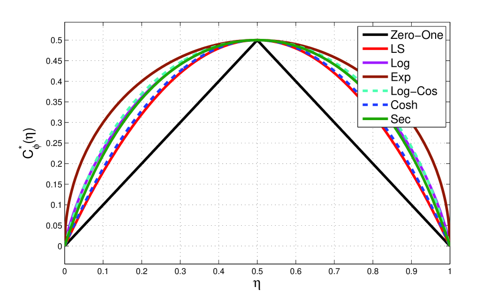
From Theorem 7 we know that when the minimum risk is computed under other $C_{\phi}^{*}$ functions, a list of which is presented in Table-2, an upper bound on the Bayes error is being computed. Also, the $C_{\phi}^{*}$ that are closer to $C_{0/1}^{*}$ result in minimum risk formulations that provide tighter bounds on the Bayes error. Figure-1 shows that $C_{LS}^{*}$ , $C_{Cosh}^{*}$ , $C_{Sec}^{*}$ , $C_{Log}^{*}$ , $C_{Log-Cos}^{*}$ and $C_{Exp}^{*}$ are in order the closest to $C_{0/1}^{*}$ and the corresponding minimum-risk formulations in Table-3 provide, in the same order, tighter bounds on the Bayes error. This can also be directly verified by noting that $R_{C_{Exp}^{*}}$ is equal to the Bhattacharyya bound Fukunaga (1990), $R_{C_{LS}^{*}}$ is equal to the asymptotic nearest neighbor bound Fukunaga (1990); Cover and Hart (1967), $R_{C_{Log}^{*}}$ is equal to the Jensen-Shannon divergence Lin (1991) and $R_{C_{Log-Cos}^{*}}$ is similar to the bound in Avi-Itzhak and Diep (1996). These four formulations have been independently studied in the literature and the fact that they produce upper bounds on the Bayes error has been directly verified. Here we have rederived these four measures by resorting to the concept of minimum risk and proper loss functions which not only allows us to provide a unified approach to these different methods but has also led to a systematic method for deriving other novel bounds on the Bayes error, namely $R_{C_{Cosh}^{*}}$ and $R_{C_{Sec}^{*}}$ .

Table 2:

C^{*}_{\phi}(\eta)

specifics used to compute the minimum-risk.

Method	$C^{*}_{\phi}(\eta)$
LS	$-2\eta(\eta-1)$
Log	$-0.7213(\eta\log(\eta)-(1-\eta)\log(1-\eta))$
Exp	$\sqrt{\eta(1-\eta)}$
Log-Cos	$(\frac{1}{2.5854})\log(\frac{\cos(2.5854(\eta-\frac{1}{2}))}{\cos(\frac{2.5854}{2})})$
Cosh	$-\cosh(1.9248(\frac{1}{2}-\eta))+\cosh(\frac{-1.9248}{2})$
Sec	$-\sec(1.6821(\frac{1}{2}-\eta))+\sec(\frac{-1.6821}{2})$

Table 3: Minimum-risk for different

C^{*}_{\phi}(\eta)

$C^{*}_{\phi}(\eta)$	$R_{C_{\phi}^{*}}$
Zero-One	Bayes Error
LS	$\int\frac{P({\bf x}\|1)P({\bf x}\|-1)}{P({\bf x}\|1)+P({\bf x}\|-1)}d{\bf x}$
Exp	$\frac{1}{2}\int\sqrt{P({\bf x}\|1)P({\bf x}\|-1)}d{\bf x}$
Log	$-\frac{0.7213}{2}D_{KL}(P({\bf x}\|1)\|\|P({\bf x}\|1)+P({\bf x}\|-1))-\frac{0.7213}{2}D_{KL}(P({\bf x}\|-1)\|\|P({\bf x}\|1)+P({\bf x}\|-1))$
Log-Cos	$\int\frac{P({\bf x}\|1)+P({\bf x}\|-1)}{2}\left[\frac{1}{2.5854}\log\left(\frac{\cos(\frac{2.5854(P({\bf x}\|1)-P({\bf x}\|-1))}{2(P({\bf x}\|1)+P({\bf x}\|-1))})}{cos(\frac{2.5854}{2})}\right)\right]d{\bf x}$
Cosh	$\int\frac{P({\bf x}\|1)+P({\bf x}\|-1)}{2}\left[-\cosh(\frac{1.9248(P({\bf x}\|-1)-P({\bf x}\|1))}{2(P({\bf x}\|1)+P({\bf x}\|-1))})+\cosh(\frac{-1.9248}{2})\right]d{\bf x}$
Sec	$\int\frac{P({\bf x}\|1)+P({\bf x}\|-1)}{2}\left[-\sec(\frac{1.6821(P({\bf x}\|-1)-P({\bf x}\|1))}{2(P({\bf x}\|1)+P({\bf x}\|-1))})+\sec(\frac{-1.6821}{2})\right]d{\bf x}$

Next, we demonstrate a general procedure for deriving a class of polynomial functions $C_{Poly-n}^{*}(\eta)$ that are increasingly and arbitrarily close to $C_{0/1}^{*}(\eta)$ .

Theorem 8

Let

\displaystyle C_{Poly-n}^{*}(\eta)=K_{2}(\int Q(\eta)d(\eta)+K_{1}\eta)

(50)

where

	$\displaystyle Q(\eta)=\int-(\eta(1-\eta))^{n}d(\eta),$		(51)
	$\displaystyle K_{1}=-Q(\frac{1}{2}),$		(52)
	$\displaystyle K_{2}=\frac{\frac{1}{2}}{\left.(\int Q(\eta)d(\eta)+K_{1}\eta)\right\|_{\eta=\frac{1}{2}}}.$		(53)

Then $R_{C_{Poly-n}^{*}}\geq R_{C_{Poly-(n+1)}^{*}}\geq R^{*}$ for all $n\geq 0$ and $R_{C_{Poly-n}^{*}}$ converges to $R^{*}$ as $n\rightarrow\infty$ .

Proof 8

See supplementary material 16.

As an example, we derive $C_{Poly-2}^{*}(\eta)$ by following the above procedure

\displaystyle{C^{*}_{Poly-2}}^{\prime\prime}(\eta)=-(\eta(1-\eta))^{2}=-(\eta^{2}+\eta^{4}-2\eta^{3}).

(54)

From this we have

\displaystyle{C_{Poly-2}^{*}}^{\prime}(\eta)=-(\frac{1}{3}\eta^{3}+\frac{1}{5}\eta^{5}-\frac{2}{4}\eta^{4})+K_{1}.

(55)

Satisfying ${C_{Poly-2}^{*}}^{\prime}(\frac{1}{2})=0$ we find $K_{1}=\frac{1}{60}$ . Therefore,

\displaystyle C_{Poly-2}^{*}(\eta)=K_{2}(-\frac{1}{12}\eta^{4}-\frac{1}{30}\eta^{6}+\frac{1}{10}\eta^{5}+\frac{1}{60}\eta).

(56)

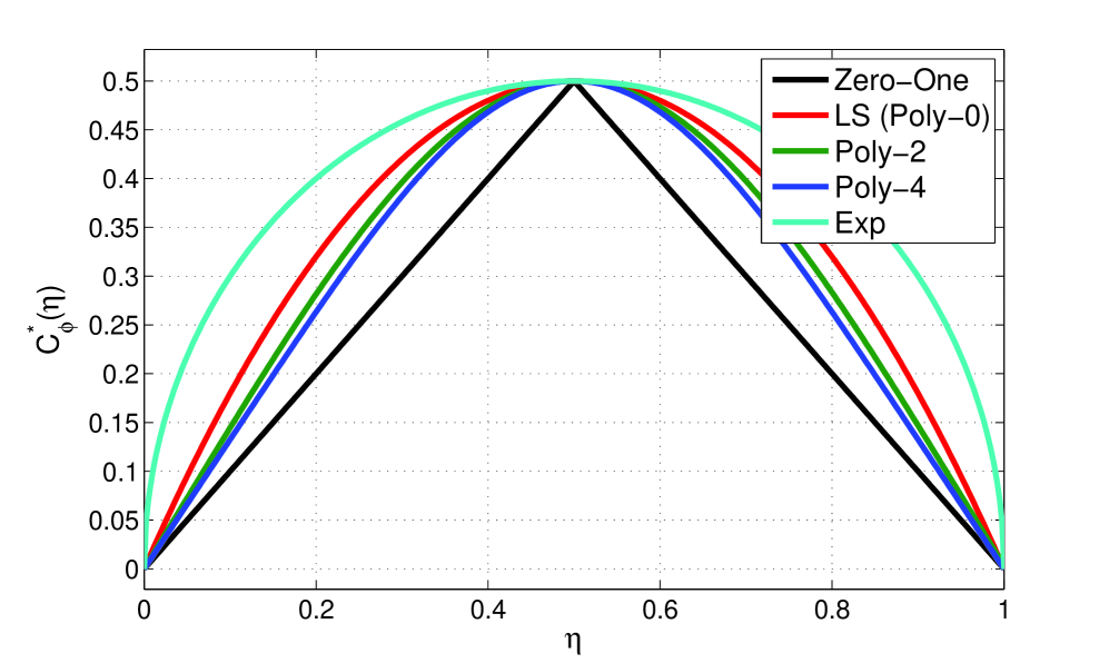
Satisfying $C_{Poly-2}^{*}(\frac{1}{2})=\frac{1}{2}$ we find $K_{2}=\frac{960}{11}$ .

Figure-2 plots $C_{Poly-2}^{*}(\eta)$ which shows that, as expected, it is a closer approximation to $C_{0/1}^{*}(\eta)$ when compared to $C_{LS}^{*}(\eta)$ . Following the same steps, it is readily shown that $C_{LS}^{*}(\eta)=C_{Poly-0}^{*}(\eta)$ , meaning that $C_{LS}^{*}(\eta)$ is derived from the special case of $n=0$ .

As we increase $n$ , we increase the order of the resulting polynomial which provides a tighter fit to $C_{0/1}^{*}(\eta)$ . Figure-2 also plots $C_{Poly-4}^{*}(\eta)$

	$\displaystyle C_{Poly-4}^{*}(\eta)=$		(57)
	$\displaystyle 1671.3(-\frac{1}{90}\eta^{10}+\frac{1}{18}\eta^{9}-\frac{3}{28}\eta^{8}+\frac{2}{21}\eta^{7}-\frac{1}{30}\eta^{6}+\frac{1}{1260}\eta)$

which is an even closer approximation to $C_{0/1}^{*}(\eta)$ . Table-4 shows the corresponding minimum-risk $R_{C_{Poly-n}^{*}}(p^{*})$ for different $C_{Poly-n}^{*}(\eta)$ functions, with $R_{C_{Poly-4}^{*}}(p^{*})$ providing the tightest bound on the Bayes error. Arbitrarily tighter bounds are possible by simply using $C_{Poly-n}^{*}(\eta)$ with larger $n$ .

Table 4: Minimum-risk for different

C_{Poly-n}^{*}(\eta)

$C^{*}_{\phi}(\eta)$	$R_{C_{\phi}^{*}}$
Zero-One	Bayes Error
Poly-0 (LS)	$\int\frac{P({\bf x}\|1)P({\bf x}\|-1)}{P({\bf x}\|1)+P({\bf x}\|-1)}d{\bf x}$
Poly-2	$\frac{K_{2}}{2}\int-\frac{P({\bf x}\|1)^{4}}{12(2P({\bf x}))^{3}}-\frac{P({\bf x}\|1)^{6}}{30(2P({\bf x}))^{5}}+\frac{P({\bf x}\|1)^{5}}{10(2P({\bf x}))^{4}}+K_{1}P({\bf x}\|1)d{\bf x}$
	$K_{1}=0.0167,K_{2}=87.0196,P({\bf x})=\frac{P({\bf x}\|1)+P({\bf x}\|-1)}{2}$
Poly-4	$\frac{K_{2}}{2}\int-\frac{P({\bf x}\|1)^{10}}{90(2P({\bf x}))^{9}}+\frac{P({\bf x}\|1)^{9}}{18(2P({\bf x}))^{8}}-\frac{3P({\bf x}\|1)^{8}}{28(2P({\bf x}))^{7}}+\frac{2P({\bf x}\|1)^{7}}{21(2P({\bf x}))^{6}}-\frac{P({\bf x}\|1)^{6}}{30(2P({\bf x}))^{5}}+K_{1}P({\bf x}\|1)d{\bf x}$
	$K_{1}=7.9365\times 10^{-4},K_{2}=1671.3,P({\bf x})=\frac{P({\bf x}\|1)+P({\bf x}\|-1)}{2}$

Such arbitrarily tight bounds on the Bayes error are important in a number of applications such as in feature selection and extraction Vasconcelos (2002); Vasconcelos and Vasconcelos (2009); Brown (2009); Peng et al. (2005), information theory Duchi and Wainwright (2013); Guntuboyina (2011); Cover and Thomas (2006); Brown and Liu. (1993), classification and regression Liu and Shum (2003); Lee et al. (2005); Friedman and Stuetzle (1981), etc. In the experiments section we specifically show how using $C^{*}_{\phi}$ with tighter bounds on the Bayes error results in better performance on a feature selection and classification problem. We then consider the effect of using projection vectors $\Phi({\bf w})$ that are more discriminative, such as the normalized kernel Fisher discriminant projection vector or normalized kernel SVM projection vector described in Lemma 1, rather than the canonical projection vector of $\Phi({\bf w})=\frac{({\bm{\mu}}_{P}-{\bm{\mu}}_{Q})}{||({\bm{\mu}}_{P}-{\bm{\mu}}_{Q})||_{\cal H}}$ . We show that these more discriminative projection vectors $\Phi({\bf w})$ result in significantly improved performance on a set of kernel hypothesis testing experiments.

6 Computing The Kernel Score and Kernel Divergence in Practice

In most applications the distributions of $P$ and $Q$ are not directly known and are solely represented through a set of sample points. We assume that the data points $\{{\bf x}_{1},...,{\bf x}_{n_{1}}\}$ are sampled from $P$ and the data points $\{{\bf x}_{1},...,{\bf x}_{n_{2}}\}$ are sampled from $Q$ . Note that the Kernel Score can be written as

\displaystyle S_{C^{*}_{\phi},k,{\cal F},{\Phi({\bf w})}}(P,Q)={\mathbf{E}}_{Z}\left[C\left(\frac{P^{p}(x^{p})}{P^{p}(x^{p})+Q^{p}(x^{p})}\right)\right],

(58)

where the expectation is over the distribution defined by $P_{Z}(z)=\frac{P^{p}(x^{p})+Q^{p}(x^{p})}{2}$ . The empirical Kernel Score and empirical Kernel Divergence can now be written as

	$\displaystyle{\hat{S}}_{C^{*}_{\phi},k,{\cal F},{\Phi({\bf w})}}(P,Q)$	$\displaystyle=$	$\displaystyle\frac{1}{n}\sum_{i=1}^{n}C\left(\frac{P^{p}(x^{p}_{i})}{P^{p}(x^{p}_{i})+Q^{p}(x^{p}_{i})}\right)$		(59)
	$\displaystyle\widehat{KD}_{C,k,{\cal F},{\Phi({\bf w})}}(P,Q)$	$\displaystyle=$	$\displaystyle\frac{1}{2}-{\hat{S}}_{C,k,{\cal F},{\Phi({\bf w})}}(P,Q),$		(60)

where $n=n_{1}+n_{2}$ and $x^{p}_{i}$ is the projection of $\Phi({\bf x}_{i})$ onto $\Phi({\bf w})$ .

Calculating $x^{p}_{i}$ in the above formulation using equation (35) is still not possible because we generally don’t know $\Phi({\bf w})$ and ${\bf w}$ . A similar problem exists for the MMD. Nevertheless the MMD Gretton et al. (2007) is estimated in practice as

			$\displaystyle\widehat{MMD}_{\cal F}(P,Q)=\|\|\hat{\bm{\mu}}_{P}-\hat{\bm{\mu}}_{Q}\|\|^{2}_{\cal H}$		(61)
		$\displaystyle=$	$\displaystyle\frac{1}{n_{1}n_{1}}\sum_{i=1}^{n_{1}}\sum_{j=1}^{n_{1}}K({\bf x}_{i}{\bf x}_{j})-\frac{2}{n_{1}n_{2}}\sum_{i=1}^{n_{1}}\sum_{j=1}^{n_{2}}K({\bf x}_{i}{\bf x}_{j})+\frac{1}{n_{2}n_{2}}\sum_{i=1}^{n_{2}}\sum_{j=1}^{n_{2}}K({\bf x}_{i}{\bf x}_{j}).$		(62)

In view of Lemma 2 the MMD can be equivalently estimated as

\displaystyle\widehat{MMD}_{\cal F}(P,Q)=(\hat{\mu}^{p}_{P}-\hat{\mu}^{p}_{Q})^{2},

(63)

where

\displaystyle\hat{\mu}^{p}_{P}=\frac{\frac{1}{n_{1}n_{1}}\sum_{i=1}^{n_{1}}\sum_{j=1}^{n_{1}}K({\bf x}_{i}{\bf x}_{j})-\frac{1}{n_{1}n_{2}}\sum_{i=1}^{n_{1}}\sum_{j=1}^{n_{2}}K({\bf x}_{i}{\bf x}_{j})}{T},

(64)

\displaystyle\hat{\mu}^{p}_{Q}=\frac{\frac{1}{n_{1}n_{2}}\sum_{i=1}^{n_{1}}\sum_{j=1}^{n_{2}}K({\bf x}_{i}{\bf x}_{j})-\frac{1}{n_{2}n_{2}}\sum_{i=1}^{n_{2}}\sum_{j=1}^{n_{2}}K({\bf x}_{i}{\bf x}_{j})}{T}

(65)

and

\displaystyle T=\sqrt{\frac{1}{n_{1}n_{1}}\sum_{i=1}^{n_{1}}\sum_{j=1}^{n_{1}}K({\bf x}_{i}{\bf x}_{j})-\frac{2}{n_{1}n_{2}}\sum_{i=1}^{n_{1}}\sum_{j=1}^{n_{2}}K({\bf x}_{i}{\bf x}_{j})+\frac{1}{n_{2}n_{2}}\sum_{i=1}^{n_{2}}\sum_{j=1}^{n_{2}}K({\bf x}_{i}{\bf x}_{j})}.

(66)

It can easily be verified that equations (63)-(66) and equation (61) are equivalent. This equivalent method for calculating the MMD can be elaborated as projecting the two embedded sample sets onto $\Phi({\bf w})=\frac{(\hat{\bm{\mu}}_{P}-\hat{\bm{\mu}}_{Q})}{||(\hat{\bm{\mu}}_{P}-\hat{\bm{\mu}}_{Q})||}$ , estimating the means $\hat{\mu}^{p}_{P}$ and $\hat{\mu}^{p}_{Q}$ of the projected embedded sample sets and then finding the distance between these estimated means. This might seem like over complicating the original procedure. Yet, it serves to show that the MMD is solely measuring the distance between the means while disregarding all the other information available regarding the projected embedded distributions. Similarly, assuming that $\Phi({\bf w})=\frac{(\hat{\bm{\mu}}_{P}-\hat{\bm{\mu}}_{Q})}{||(\hat{\bm{\mu}}_{P}-\hat{\bm{\mu}}_{Q})||}$ , $x^{p}_{i}$ can now be estimated as

$\displaystyle x^{p}_{i}$	$\displaystyle\!\!\!\!\!\!=<\Phi({\bf x}_{i}),{\bf w}>=<\Phi({\bf x}_{i}),\frac{({\hat{\bm{\mu}}_{P}}-{\hat{\bm{\mu}}_{Q}})}{\|\|({\hat{\bm{\mu}}_{P}}-{\hat{\bm{\mu}}_{Q}})\|\|}>$	(69)
	$\displaystyle=\frac{<\Phi({\bf x}_{i}),{\hat{\bm{\mu}}_{P}}>-<\Phi({\bf x}_{i}),{\hat{\bm{\mu}}_{Q}}>}{\|\|({\hat{\bm{\mu}}_{P}}-{\hat{\bm{\mu}}_{Q}})\|\|}$
	$\displaystyle=\frac{\frac{1}{n_{1}}\sum_{j=1}^{n_{1}}<\Phi({\bf x}_{i}),\Phi({\bf x}_{j})>-\frac{1}{n_{2}}\sum_{j=1}^{n_{2}}<\Phi({\bf x}_{i}),\Phi({\bf x}_{j})>}{T}$
	$\displaystyle=\frac{\frac{1}{n_{1}}\sum_{j=1}^{n_{1}}K({\bf x}_{i},{\bf x}_{j})-\frac{1}{n_{2}}\sum_{j=1}^{n_{2}}K({\bf x}_{i},{\bf x}_{j})}{T}.$	(70)

Once the $x^{p}_{i}$ are found for all $i$ using equation (70), estimating other statistics such as the variance is trivial. For example, the variances of the projected embedded distributions can now be estimated as

	$\displaystyle(\hat{\sigma}^{p}_{P})^{2}=\frac{1}{n_{1}}\sum_{i=1}^{n_{1}}(x^{p}_{i}-\hat{\mu}^{p}_{P})^{2}$		(71)
	$\displaystyle(\hat{\sigma}^{p}_{Q})^{2}=\frac{1}{n_{2}}\sum_{i=1}^{n_{2}}(x^{p}_{i}-\hat{\mu}^{p}_{Q})^{2}.$		(72)

In light of this, the empirical Bhattacharyya Kernel Score and empirical Bhattacharyya Kernel Divergence can now be readily calculated in practice as

	$\displaystyle\hat{S}_{C,k,{\cal F},{\Phi({\bf w})}}(P,Q)=\frac{1}{2}\cdot e^{(B)},$		(73)
	$\displaystyle\widehat{KD}_{C_{Exp},k,{\cal F},{\Phi({\bf w})}}(P,Q)=\frac{1}{2}-\frac{1}{2}\cdot e^{(B)},$		(74)
	$\displaystyle\hat{B}=\frac{1}{4}\log\left(\frac{1}{4}\left(\frac{(\hat{\sigma}^{p}_{P})^{2}}{(\hat{\sigma}^{p}_{Q})^{2}}+\frac{(\hat{\sigma}^{p}_{Q})^{2}}{(\hat{\sigma}^{p}_{P})^{2}}+2\right)\right)+\frac{1}{4}\left(\frac{(\hat{\mu}^{p}_{P}-\hat{\mu}^{p}_{Q})^{2}}{(\hat{\sigma}^{p}_{P})^{2}+(\hat{\sigma}^{p}_{Q})^{2}}\right).$		(75)

Finally, the empirical Kernel Score of equation (59) and the empirical Kernel Divergence of equation (60) can be calculated in practice after finding $P^{p}(x^{p}_{i})$ and $Q^{p}(x^{p}_{i})$ using any one dimensional probability model.

Note that in the above formulations we used the canonical $\Phi({\bf w})=\frac{(\hat{\bm{\mu}}_{P}-\hat{\bm{\mu}}_{Q})}{||(\hat{\bm{\mu}}_{P}-\hat{\bm{\mu}}_{Q})||}$ . A similar approach is possible for other valid choices of $\Phi({\bf w})$ . Namely, the projection vector $\Phi({\bf w})$ associated with the kernel Fisher discriminant can be found in the form of

\displaystyle\Phi({\bf w})=\sum_{j=1}^{n}\alpha_{j}\Phi({\bf x}_{j})

(76)

using Algorithm 5.16 in Shawe-Taylor and Cristianini (2004). In this case $x^{p}_{i}$ can be found as

\displaystyle x^{p}_{i}=\frac{<\Phi({\bf w}),\Phi({\bf x}_{i})>}{||\Phi({\bf w})||}=\frac{\sum_{j=1}^{n}\alpha_{j}K({\bf x}_{i},{\bf x}_{j})}{||\Phi({\bf w})||},

(77)

where

\displaystyle||\Phi({\bf w})||=\sqrt{\sum_{i=1}^{n}\sum_{j=1}^{n}\alpha_{i}\alpha_{j}K({\bf x}_{i},{\bf x}_{j})}.

(78)

The projection vector $\Phi({\bf w})$ associated with the kernel SVM can also be found in the form of

\displaystyle\Phi({\bf w})=\sum_{j\in SV}\alpha_{j}\phi({\bf x_{j}})

(79)

using standard algorithms Bottou and Lin (2007); Ben-Hur and Weston (2010), where $SV$ is the set of support vectors. In this case the $x^{p}_{i}$ can be found using equation (77) calculated over the support vectors.

7 One-Class Classifier for Kernel Hypothesis Testing

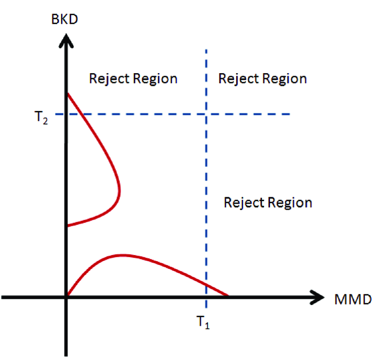
From Theorem 4 we conclude that the Kernel Divergence is injective similar to the MMD. This means that the Kernel Divergence can be directly thresholded and used in hypothesis testing. We showed that while the MMD simply measures the distance between the means of the projected embedded distributions, the Bhattacharyya Kernel Divergence (BKD) incorporates information about both the means and variances of the two projected embedded distributions. We also showed that in general the Kernel Divergence (KD) provides a measure related to the minimum risk of the two projected embedded distributions. Each one of these measures takes into account a different aspect of the two projected embedded distributions in relation to each other. We can integrate all of these measures into our hypothesis test by constructing a vector where each element is a different measure and learn a one-class classifier for this vector. In the hypothesis testing experiments of Section 8.2, we constructed the vectors [MMD, KD] and [MMD, BKD] and implemented a simple one-class nearest neighbor classifier with infinity norm (Tax, 2001) as depicted in Figure 3.

8 Experiments

In this section we include various experiments that confirm different theoretical aspects of the Kernel Score and Kernel Divergence.

8.1 Feature selection experiments

Different bounds on the Bayes error are used in feature selection and ranking algorithms Vasconcelos (2002); Vasconcelos and Vasconcelos (2009); Brown (2009); Peng et al. (2005); Duch et al. (2004). In this section we show that the tighter bounds we have derived, namely $C^{*}_{Poly-2}$ and $C^{*}_{Poly-4}$ , allow for improved feature selection and ranking. The experiments used ten binary UCI data sets of relatively small size: (#1) Habermanӳ survival,(#2) original Wisconsin breast cancer , (#3) tic-tac-toe , (#4) sonar, (#5) Pima-diabetes , (#6) liver disorder , (#7) Cleveland heart disease , (#8) echo-cardiogram , (#9) breast cancer prognostic, and (#10) breast cancer diagnostic.

Each data set was split into five folds, four of which were used for training and one for testing. This created five train-test pairs per data set, over which the results were averaged. The original data was augmented with noisy features. This was done by taking each feature and adding random scaled noise to a certain percentage of the data points. The scale parameters were $\{0.1,0.3\}$ and the percentage of data points that were randomly affected was $\{0.25,0.50,0.75\}$ . Specifically, for each feature, a percentage of the data points had scaled zero mean Gaussian noise added to that feature in the form of

\displaystyle{\bf x}_{i}={\bf x}_{i}+{\bf x}_{i}\cdot{y}\cdot s,

(80)

where ${\bf x}_{i}$ is the $i$ -th feature of the original data vector, ${y}\in N(0,1)$ is the Gaussian noise and $s$ is the scale parameter. The empirical minimum risk was then computed for each feature where $P_{{\bf X}|Y}({\bf x}|y)$ was modeled as a $10$ bin histogram.

A greedy feature selection algorithm was implemented in which the features were ranked according to their empirical minimum risk and the highest ranked $5\%$ and $10\%$ of the features were selected. The selected features were then used to train and test a linear SVM classifier. If a certain minimum risk $C^{*}_{\phi}$ is a better bound on the Bayes error, we would expect it to choose better features and these better features should translate into a better SVM classifier with smaller error rate on the test data. Five different $C^{*}_{\phi}$ were considered namely $C^{*}_{Poly-4}$ , $C^{*}_{Poly-2}$ , $C^{*}_{LS}$ , $C^{*}_{Log}$ and $C^{*}_{Exp}$ and the error rate corresponding to each $C^{*}_{\phi}$ was computed and averaged over the five folds. The average error rates were then ranked such that a rank of $1$ was assigned to the $C^{*}_{\phi}$ with smallest error and a rank of $5$ assigned to the $C^{*}_{\phi}$ with largest error.

The rank over selected features was computed by averaging the ranks found by using both $5\%$ and $10\%$ of the highest ranked features. This process was repeated a total of $25$ times for each UCI data set and the over all average rank was found by averaging over the $25$ experiment runs. The over all average rank found for each UCI data set and each $C^{*}_{\phi}$ is reported in Table-5. The last two columns of this table are the total number of times each $C^{*}_{\phi}$ has had the best rank over the ten different data sets (#W) and a ranking of the over all average rank computed for each data set and then averaged across all data sets (Rank). It can be seen that $C^{*}_{Poly-4}$ which was designed to have the tightest bound on the Bayes error has the most number of wins of $4$ and smallest Rank of $2.4$ while $C^{*}_{Exp}$ which has the loosest bound on the Bayes error has the least number of wins of $0$ and worst Rank of $3.75$ . As expected, the Rank for each $C^{*}_{\phi}$ is in order of how tightly they approximate the Bayes error with in order $C^{*}_{Poly-4}$ , $C^{*}_{Poly-2}$ and $C^{*}_{LS}$ at the top and $C^{*}_{Log}$ and $C^{*}_{Exp}$ at the bottom. This is in accordance with the discussion of Section 5.0.1.

Table 5: The over all average rank for each UCI data set and each

C^{*}_{\phi}

$C^{*}_{\phi}$	#1	#2	#3	#4	#5	#6	#7	#8	#9	#10	#W	Rank
$C^{*}_{Poly-4}$	2.9	2.75	3.62	2.77	2.86	2.39	3.55	2.87	3.25	2.86	4	2.4
$C^{*}_{Poly-2}$	2.82	2.88	3.37	2.62	2.87	2.74	3.27	2.9	3.46	2.98	2	2.7
$C^{*}_{LS}$	3.02	2.73	2.92	3.03	2.9	3.17	2.65	2.96	2.97	3.16	2	2.8
$C^{*}_{Log}$	3.16	3.32	2.5	3.44	3.0	3.2	2.78	3.08	2.62	2.88	2	3.35
$C^{*}_{Exp}$	3.1	3.32	2.59	3.14	3.37	3.5	2.75	3.19	2.7	3.12	0	3.75

8.2 Kernel Hypothesis Testing Experiments

The first set of experiments comprised of hypothesis tests on Gaussian samples. Specifically, two hypothesis tests were considered. In the first test, we used $250$ samples for each $25$ dimensional Gaussian distribution ${\mathcal{N}}(0,1.5I)$ and ${\mathcal{N}}(0,1.7I)$ . Note that the means are equal and the variances are slightly different. In the second test, we used $250$ samples for each $25$ dimensional Gaussian distribution ${\mathcal{N}}(0,1.5I)$ and ${\mathcal{N}}(0.1,1.5I)$ . Note that the variances are equal and the means are slightly different. In both cases the reject thresholds were found from $100$ bootstrap iterations for a fixed type-I error of $\alpha=0.05$ . We used the Gaussian kernel embedding for all experiments and the kernel parameter was found using the median heuristic of Gretton et al. (2007). Also, the Kernel Divergence (KD) used $C^{*}_{Poly-4}$ of equation (57) and one dimensional Gaussian distribution models. Unlike the classification problem described in the previous section, having a tight estimate of the Bayes error is not important for hypothesis testing experiments and so the actual concave $C$ function used is not crucial. The type-II error test results for $100$ repetitions are reported in Table 6 for the MMD, BKD, KD methods, where ${\Phi(\bf w})=\frac{({{\bm{\mu}}_{P}}-{{\bm{\mu}}_{Q}})}{||({{\bm{\mu}}_{P}}-{{\bm{\mu}}_{Q}})||}$ , along with the combined method described in Section 7 where a one-class nearest neighbor classifier with infinity norm is learned for [MMD, KD] and [MMD, BKD]. These results are typical and in general (a) the KD and BKD methods do better than the MMD when the means are equal and the variances are different, (b) the MMD does better than the KD and BKD when the variances are equal and the means are different and (c) The combined methods of [MMD, KD] and [MMD, BKD] do well for both cases. We usually don’t know which case we are dealing with in practice and so the combined methods of [MMD, KD] and [MMD, BKD] are preferred.

Table 6: Percentage of type-II error for the hypothesis tests on two types of Gaussian samples given

\alpha=0.05

Method	$\sigma_{1}=1.5$ , $\sigma_{2}=1.7$	$\mu_{1}=0$ , $\mu_{2}=0.1$
	$\mu_{1}=\mu_{2}=0$	$\sigma_{1}=\sigma_{2}=1.5$
MMD	46	25
KD	13	42
BKD	11	40
[MMD, KD]	13	25
[MMD, BKD]	12	24

8.2.1 Bench-Mark Gene Data Sets

Next we evaluated the proposed methods on a group of high dimensional bench-mark gene data sets. The data sets are detailed in Table 7 and are challenging given their small sample size and high dimensionality. The hypothesis testing involved splitting the positive samples in two and using the first half to learn the reject thresholds from $1000$ bootstrap iterations for a fixed type-I error of $\alpha=0.05$ . We used the Gaussian kernel embedding for all experiments and the kernel parameter was found using the median heuristic of Gretton et al. (2007). The Kernel Divergence (KD) used $C^{*}_{Poly-4}$ of equation (57) and one dimensional Gaussian distribution models. The type-II error test results for $1000$ repetitions are reported in Table 8 for the MMD, BKD, KD, [MMD, KD] and [MMD, BKD] methods. Also, three projection directions are considered namely, MEANS where $\Phi({\bf w})=\frac{({{\bm{\mu}}_{P}}-{{\bm{\mu}}_{Q}})}{||({{\bm{\mu}}_{P}}-{{\bm{\mu}}_{Q}})||}$ , FISHER where the $\Phi({\bf w})$ associated with the kernel Fisher linear discriminant is used, and SVM where the $\Phi({\bf w})$ associated with the kernel SVM is used.

We have reported the rank of each method among the five methods with the same projection direction under RANK1 and the overall rank among all fifteen methods under RANK2 in the last column. Note that the first row of Table 8 with MMD distance measure and MEANS projection direction is the only method previously proposed in the literature Gretton et al. (2012). We should also note that the KD with FISHER projection direction encountered numerical problems in the form of very small variance estimates, which resulted in poor performance. Nevertheless, we can see that in general the KD and BKD methods which incorporate more information regarding the projected distributions, outperform the MMD. Second, using more discriminant projection directions like the FISHER or SVM outperform simply projecting onto MEANS. Finally, the [MMD, KD] and [MMD, BKD] methods that combine the information provided by both the MMD and the KD or BKD have the lowest ranks. Specifically, the [MMD, KD] with SVM projection direction has the overall lowest rank among all fifteen methods.

Table 7: Gene data set details.

Number	Data Set	#Positives	#Negatives	#Dimensions
#1	Lung Cancer Womenӳ Hospital	31	150	12533
#2	Lukemia	25	47	7129
#3	Lymphoma Harvard Outcome	26	32	7129
#4	Lymphoma Harvard	19	58	7129
#5	Central Nervous System Tumor	21	39	7129
#6	Colon Tumor	22	40	2000
#7	Breast Cancer ER	25	24	7129

Table 8: Percentage of type-II error for the gene data sets given

\alpha=0.05

. RANK1 is the rank of each method among the five methods with the same projection direction and RANK2 is the overall rank among all fifteen methods.

Projection	Measure	#7	#6	#5	#4	#3	#2	#1	Rank1	Rank2
MEANS	MMD	24.3	27.4	95	31.2	90.8	11.7	6.3	3.42	9.14
MEANS	KD	9.8	58.5	83.8	53.1	79.2	64.7	7.7	3.71	10.14
MEANS	BKD	12	56.9	83.4	52.5	79.3	58.0	3.7	3.14	9.14
MEANS	[MMD, KD]	12.2	48	82.9	25.2	84.1	14.7	3.0	2.57	7.42
MEANS	[MMD, BKD]	13.2	47.3	81.9	24.3	83.6	14.0	3.2	2.14	6.42
FISHER	MMD	5.8	26.5	90.2	24.8	83.1	14.1	4.2	1.78	6.07
FISHER	KD	100	100	100	100	100	100	100	5	15
FISHER	BKD	30.6	52.4	82.4	66.0	64.0	73.3	22.6	3.14	10.28
FISHER	[MMD, KD]	9.6	26.5	95.3	31.9	93.6	18.7	5.4	3.14	9.42
FISHER	[MMD, BKD]	6.2	26.4	82.8	31.0	74.9	18.6	5.4	1.92	5.21
SVM	MMD	22.8	29.9	95.1	26.2	89.2	10.0	2.1	3.85	8.00
SVM	KD	4.0	48.2	81.3	33.4	82.4	41.1	1.0	3.28	6.42
SVM	BKD	4.3	44.2	86.3	32.0	79.4	34.4	0.5	2.85	6.57
SVM	[MMD, KD]	6.3	28.1	88.4	20.5	86.4	13.7	0.4	2.28	5.14
SVM	[MMD, BKD]	6.6	28.2	89.0	20.5	84.9	13.8	0.4	2.71	5.57

9 Conclusion

While we have concentrated on the hypothesis testing problem in the experiments section, we envision many different applications for the Kernel Score and Kernel Divergence. We showed that the MMD is a special case of the Kernel Score and so the Kernel Score can now be used in all other applications based on the MMD, such as integrating biological data, imitation learning, etc. We also showed that the Kernel Score is related to the minimum risk of the projected embedded distributions and we showed how to derive tighter bounds on the Bayes error. Many applications that are based on risk minimization, bounds on the Bayes error or divergence measures such as classification, regression, feature selection, estimation, information theory etc, can now use the Kernel Score and Kernel Divergence to their benefit. We presented the Kernel Score as a general formulation for a score function in the Reproducing Kernel Hilbert Space and considered when it has the important property of being strictly proper. The Kernel Score is thus also directly applicable to probability elicitation, forecasting, finance and meteorology which rely on strictly proper scoring rules.

SUPPLEMENTARY MATERIAL

10 Proof of Theorem 4

If $P=Q$ then

\displaystyle KD_{C,k,{\cal F},{\Phi({\bf w})}}(P,Q)=-\int P^{p}(z)C(\frac{1}{2})dz+\frac{1}{2}=-\frac{1}{2}\int P^{p}(z)dz+\frac{1}{2}=0.

(81)

Next, we prove the converse. The proof is identical to Theorem 5 of Gretton et al. (2012) up to the point where we must prove that if $KD_{C,k,{\cal F},{\Phi({\bf w})}}(P,Q)=0$ then ${\bm{\mu}}_{P}={\bm{\mu}}_{Q}$ . To show this we write

\displaystyle KD_{C,k,{\cal F},{\Phi({\bf w})}}(P,Q)=-\int\left(\frac{P^{p}(z)+Q^{p}(z)}{2}\right)C\left(\frac{P^{p}(z)}{P^{p}(z)+Q^{p}(z)}\right)dz+\frac{1}{2}=0

(82)

\displaystyle\int\left(\frac{P^{p}(z)+Q^{p}(z)}{2}\right)C\left(\frac{P^{p}(z)}{P^{p}(z)+Q^{p}(z)}\right)dz=\frac{1}{2}.

(83)

Since $C(\eta)$ is concave and has a maximum value of $\frac{1}{2}$ at $\eta=\frac{1}{2}$ then the above equation can only hold if

\displaystyle C\left(\frac{P^{p}(z)}{P^{p}(z)+Q^{p}(z)}\right)=\frac{1}{2},

(84)

which means that

\displaystyle\frac{P^{p}(z)}{P^{p}(z)+Q^{p}(z)}=\frac{1}{2},

(85)

and so

\displaystyle P^{p}(z)=Q^{p}(z).

(86)

From this we conclude that their associated means must be equal, namely

\displaystyle\mu^{p}_{P}=\mu^{p}_{Q}.

(87)

The above equation can be written as

\displaystyle<{\bm{\mu}}_{P},\Phi({\bf w})>_{\cal H}=<{\bm{\mu}}_{Q},\Phi({\bf w})>_{\cal H}

(88)

or equivalently as

\displaystyle<{\bm{\mu}}_{P}-{\bm{\mu}}_{P},\Phi({\bf w})>_{\cal H}=0.

(89)

Since $\Phi({\bf w})$ is not in the orthogonal compliment of ${\bm{\mu}}_{P}-{\bm{\mu}}_{P}$ then it must be that

\displaystyle{\bm{\mu}}_{P}={\bm{\mu}}_{Q}.

(90)

The rest of the proof is again identical to Theorem 5 of Gretton et al. (2012) and the theorem is similarly proven.

To prove that the Kernel Score is strictly proper we note that if $P=Q$ then $KD_{C,k,{\cal F},{\Phi({\bf w})}}(Q,Q)=0$ and so $S_{C,k,{\cal F},{\Phi({\bf w})}}(Q,Q)=\frac{1}{2}$ . This means that we need to show that $S_{C,k,{\cal F},{\Phi({\bf w})}}(Q,Q)=\frac{1}{2}\geq S_{C,k,{\cal F},{\Phi({\bf w})}}(P,Q)$ . This readily follows since $C(\eta)$ is strictly concave with maximum at $C(\frac{1}{2})=\frac{1}{2}$ .

11 Proof of Lemma 1

$\Phi({\bf w})=\frac{({\bm{\mu}}_{P}-{\bm{\mu}}_{Q})}{||({\bm{\mu}}_{P}-{\bm{\mu}}_{Q})||_{\cal H}}$ is not in the orthogonal compliment of $M=\{{\bm{\mu}}_{P}-{\bm{\mu}}_{Q}\}$ since

\displaystyle<\frac{({\bm{\mu}}_{P}-{\bm{\mu}}_{Q})}{||({\bm{\mu}}_{P}-{\bm{\mu}}_{Q})||_{\cal H}},{\bm{\mu}}_{P}-{\bm{\mu}}_{Q}>_{\cal H}\neq 0.

(91)

The $\Phi({\bf w})$ equal to the kernel Fisher discriminant projection vector is not in the orthogonal compliment of $M=\{{\bm{\mu}}_{P}-{\bm{\mu}}_{Q}\}$ because if it were then the kernel Fisher discriminant objective, which can be written as $\frac{\mu^{p}_{P}-\mu^{p}_{Q}}{(\sigma^{p}_{P})^{2}+(\sigma^{p}_{Q})^{2}}$ , would not be maximized and would instead be equal to zero.

The $\Phi({\bf w})$ equal to the kernel SVM projection vector is not in the orthogonal compliment of $M=\{{\bm{\mu}}_{P}-{\bm{\mu}}_{Q}\}$ since the kernel SVM is equivalent to the kernel Fisher discriminant computed on the set of support vectors Shashua (1999).

12 Proof of Lemma 2

We know that $\mu^{p}_{P}$ is the projection of ${\bm{\mu}}_{P}$ onto $\Phi({\bf w})$ so we can write

\displaystyle\mu^{p}_{P}=<{\bm{\mu}}_{P},\Phi({\bf w})>_{\cal H}=<{\bm{\mu}}_{P},\frac{({\bm{\mu}}_{P}-{\bm{\mu}}_{Q})}{||({\bm{\mu}}_{P}-{\bm{\mu}}_{Q})||_{\cal H}}>_{\cal H}=\frac{<{\bm{\mu}}_{P},{\bm{\mu}}_{P}>_{\cal H}-<{\bm{\mu}}_{P},{\bm{\mu}}_{Q}>_{\cal H}}{||({\bm{\mu}}_{P}-{\bm{\mu}}_{Q})||_{\cal H}}

(92)

Similarly,

\displaystyle\mu^{p}_{Q}=<{\bm{\mu}}_{Q},\Phi({\bf w})>_{\cal H}=<{\bm{\mu}}_{Q},\frac{({\bm{\mu}}_{P}-{\bm{\mu}}_{Q})}{||({\bm{\mu}}_{P}-{\bm{\mu}}_{Q})||_{\cal H}}>_{\cal H}=\frac{<{\bm{\mu}}_{Q},{\bm{\mu}}_{P}>_{\cal H}-<{\bm{\mu}}_{Q},{\bm{\mu}}_{Q}>_{\cal H}}{||({\bm{\mu}}_{P}-{\bm{\mu}}_{Q})||_{\cal H}}.

(93)

Hence,

	$\displaystyle(\mu^{p}_{P}-\mu^{p}_{Q})^{2}=\left(\frac{<{\bm{\mu}}_{P},{\bm{\mu}}_{P}>_{\cal H}-2<{\bm{\mu}}_{P},{\bm{\mu}}_{Q}>_{\cal H}+<{\bm{\mu}}_{Q},{\bm{\mu}}_{Q}>_{\cal H}}{\|\|({\bm{\mu}}_{P}-{\bm{\mu}}_{Q})\|\|_{\cal H}}\right)^{2}$		(94)
	$\displaystyle=\left(\frac{<({\bm{\mu}}_{P}-{\bm{\mu}}_{Q}),({\bm{\mu}}_{P}-{\bm{\mu}}_{Q})>_{\cal H}}{\|\|({\bm{\mu}}_{P}-{\bm{\mu}}_{Q})\|\|_{\cal H}}\right)^{2}=\left(\frac{\|\|({\bm{\mu}}_{P}-{\bm{\mu}}_{Q})\|\|_{\cal H}^{2}}{\|\|({\bm{\mu}}_{P}-{\bm{\mu}}_{Q})\|\|_{\cal H}}\right)^{2}=\|\|({\bm{\mu}}_{P}-{\bm{\mu}}_{Q})\|\|_{\cal H}^{2}.$		(95)

13 Proof of Theorem 5

The result readily follows by setting $MMD_{\cal F}(P,Q)=(\mu^{p}_{P}-\mu^{p}_{Q})^{2}$ and $\sigma^{p}_{P}=\sigma^{p}_{Q}$ into equation (40).

14 Proof of Lemma 3

By adding and subtracting $\int_{\bf x}P_{{\bf X}}({\bf x})\left[P_{{\bf Y}|{\bf X}}(1|{\bf x})\phi({p^{*}}({\bf x}))+P_{{\bf Y}|{\bf X}}(-1|{\bf x})\phi(-{p^{*}}({\bf x}))\right]d{\bf x}$ and considering equation (27), the risk $R({\hat{p}^{*}})$ can be written as

$\displaystyle R({\hat{p}^{*}})$	$\displaystyle=$	$\displaystyle E_{{\bf X},Y}[\phi(y{\hat{p}^{}}({\bf x}))]=\int_{\bf x}P_{{\bf X}}({\bf x})\sum_{y}P_{{\bf Y}\|{\bf X}}(y\|{\bf x})\phi(y{\hat{p}^{}}({\bf x}))d{\bf x}$
	$\displaystyle=$	$\displaystyle\int_{\bf x}P_{{\bf X}}({\bf x})\left[P_{{\bf Y}\|{\bf X}}(1\|{\bf x})\phi({\hat{p}^{}}({\bf x}))+P_{{\bf Y}\|{\bf X}}(-1\|{\bf x})\phi(-{\hat{p}^{}}({\bf x}))\right]d{\bf x}$
	$\displaystyle=$	$\displaystyle\int_{\bf x}P_{{\bf X}}({\bf x})\left[P_{{\bf Y}\|{\bf X}}(1\|{\bf x})\left(\phi({\hat{p}^{}}({\bf x}))-\phi({p^{}}({\bf x}))\right)+P_{{\bf Y}\|{\bf X}}(-1\|{\bf x})\left(\phi(-{\hat{p}^{}}({\bf x}))-\phi(-{p^{}}({\bf x}))\right)\right]d{\bf x}$
	$\displaystyle+$	$\displaystyle\int_{\bf x}P_{{\bf X}}({\bf x})\left[P_{{\bf Y}\|{\bf X}}(1\|{\bf x})\phi({p^{}}({\bf x}))+P_{{\bf Y}\|{\bf X}}(-1\|{\bf x})\phi(-{p^{}}({\bf x}))\right]d{\bf x}$
	$\displaystyle=$	$\displaystyle R_{Calibration}+R({p^{*}}).$	(97)

The first term denoted $R_{Calibration}$ is obviously zero if we have a perfectly calibrated predictor such that ${\hat{p}^{*}}({\bf x})={p^{*}}({\bf x})$ for all ${\bf x}$ and is thus a measure of calibration. Finally, using equation $\eta({\bf x})=P_{Y|{\bf X}}(1|{\bf x})={[f_{\phi}^{*}]}^{-1}(p^{*}({\bf x}))$ and Theorem 2, the minimum risk term $R({p^{*}})$ can be written as

	$\displaystyle R({p^{}})=\int_{\bf x}P_{{\bf X}}({\bf x})\left[P_{{\bf Y}\|{\bf X}}(1\|{\bf x})\phi({p^{}}({\bf x}))+P_{{\bf Y}\|{\bf X}}(-1\|{\bf x})\phi(-{p^{*}}({\bf x}))\right]d{\bf x}$	(98)
$\displaystyle=$	$\displaystyle\int_{\bf x}P_{{\bf X}}({\bf x})[\eta({\bf x})C_{\phi}^{}(\eta({\bf x}))+\eta({\bf x})(1-\eta({\bf x}))[C_{\phi}^{}]^{\prime}(\eta({\bf x}))$	(99)
$\displaystyle+$	$\displaystyle(1-\eta({\bf x}))C_{\phi}^{}((1-\eta({\bf x})))+(1-\eta({\bf x}))(\eta({\bf x}))[C_{\phi}^{}]^{\prime}((1-\eta({\bf x})))]d{\bf x}$	(100)
$\displaystyle=$	$\displaystyle\int_{\bf x}P_{{\bf X}}({\bf x})[\eta({\bf x})C_{\phi}^{}(\eta({\bf x}))+\eta({\bf x})(1-\eta({\bf x}))[C_{\phi}^{}]^{\prime}\left(\eta({\bf x})\right)$	(101)
$\displaystyle+$	$\displaystyle C_{\phi}^{}(\eta({\bf x}))-\eta({\bf x})C_{\phi}^{}(\eta({\bf x}))-\eta({\bf x})(1-\eta({\bf x}))[C_{\phi}^{*}]^{\prime}\left(\eta({\bf x})\right)]d{\bf x}$	(102)
$\displaystyle=$	$\displaystyle\int_{\bf x}P_{{\bf X}}({\bf x})C_{\phi}^{*}(\eta({\bf x}))d{\bf x}$	(103)
$\displaystyle=$	$\displaystyle\int_{\bf x}P_{{\bf X}}({\bf x})C_{\phi}^{}({[f_{\phi}^{}]}^{-1}(p^{*}({\bf x})))d{\bf x}$	(104)
$\displaystyle=$	$\displaystyle\int_{\bf x}P_{{\bf X}}({\bf x})C_{\phi}^{*}(P_{Y\|{\bf X}}(1\|{\bf x}))d{\bf x}$	(105)

15 Proof of Theorem 6

Assuming equal priors $P_{Y}(1)=P_{Y}(-1)=\frac{1}{2}$ ,

\displaystyle P_{{\bf X}}({\bf x})=\frac{P_{{\bf X}|Y}({\bf x}|1)+P_{{\bf X}|Y}({\bf x}|-1)}{2}

(107)

and

\displaystyle P_{Y|{\bf X}}(1|{\bf x})=\frac{P_{{\bf X}|Y}({\bf x}|1)}{P_{{\bf X}|Y}({\bf x}|1)+P_{{\bf X}|Y}({\bf x}|-1)}.

(108)

We can now write the minimum risk as

\displaystyle R({p^{*}})=\int_{X}\left(\frac{P_{{\bf X}|Y}({\bf x}|1)+P_{{\bf X}|Y}({\bf x}|-1)}{2}\right)C_{\phi}^{*}\left(\frac{P_{{\bf X}|Y}({\bf x}|1)}{P_{{\bf X}|Y}({\bf x}|1)+P_{{\bf X}|Y}({\bf x}|-1)}\right)d{\bf x}

(109)

Equation (48) readily follows by setting $P_{{\bf X}|Y}({\bf x}|1)=P^{p}$ and $P_{{\bf X}|Y}({\bf x}|-1)=Q^{p}$ , in which case $R({p^{*}})$ is $R^{p}({p^{*}})$ .

16 Proof of Theorem 8

The symmetry requirement of $C_{\phi}^{*}(\eta)=C_{\phi}^{*}(1-\eta)$ results in a similar requirement on the second derivative ${C_{\phi}^{*}}^{\prime\prime}(\eta)={C_{\phi}^{*}}^{\prime\prime}(1-\eta)$ and concavity requires that the second derivative satisfy ${C_{\phi}^{*}}^{\prime\prime}(\eta)<0$ . The symmetry and concavity constraints can both be satisfied by considering

\displaystyle{C_{Poly-n}^{*}}^{\prime\prime}(\eta)\propto-(\eta(1-\eta))^{n}.

(110)

From this we write

\displaystyle{C_{Poly-n}^{*}}^{\prime}(\eta)\propto\int-(\eta(1-\eta))^{n}d(\eta)+K_{1}=Q(\eta)+K_{1}.

(111)

Satisfying the constraint that ${C_{Poly-n}^{*}}^{\prime}(\frac{1}{2})=0$ , we find $K_{1}$ as

\displaystyle K_{1}=-Q(\frac{1}{2}).

(112)

Finally, $C_{Poly-n}^{*}(\eta)$ is

\displaystyle C_{Poly-n}^{*}(\eta)=K_{2}(\int Q(\eta)d(\eta)+K_{1}\eta),

(113)

where

\displaystyle K_{2}=\frac{\frac{1}{2}}{\left.(\int Q(\eta)d(\eta)+K_{1}\eta)\right|_{\eta=\frac{1}{2}}}

(114)

is a scaling factor such that $C_{Poly-n}^{*}(\frac{1}{2})=\frac{1}{2}$ . $C_{Poly-n}^{*}(\eta)$ meets all the requirements of Theorem 7 so $C_{Poly-n}^{*}(\eta)\geq C_{0/1}^{*}(\eta)$ for all $\eta\in[0~1]$ and $R_{C_{Poly-n}^{*}}\geq R^{*}$ .

Next, we need to prove that if we follow the above procedure for $n+1$ and find $C_{Poly-(n+1)}^{*}(\eta)$ then $R_{C_{Poly-n}^{*}}\geq R_{C_{Poly-(n+1)}^{*}}$ . We accomplish this by showing that $C_{Poly-n}^{*}(\eta)\geq C_{Poly-(n+1)}^{*}(\eta)$ . Without loss of generality, let

\displaystyle{C_{Poly-n}^{*}}^{\prime\prime}(\eta)=-(\eta(1-\eta))^{n}

(115)

and

\displaystyle{C_{Poly-(n+1)}^{*}}^{\prime\prime}(\eta)=-(\eta(1-\eta))^{n+1}

(116)

then ${C_{Poly-n}^{*}}^{\prime\prime}(\eta)\leq{C_{Poly-(n+1)}^{*}}^{\prime\prime}(\eta)$ since $\eta\in[0~1]$ . Also, since ${C_{Poly-n}^{*}}^{\prime\prime}(\eta)<0$ and ${C_{Poly-n}^{*}}^{\prime\prime}(\eta)={C_{Poly-n}^{*}}^{\prime\prime}(1-\eta)$ then ${C_{Poly-n}^{*}}^{\prime}(\eta)$ is a monotonically decreasing function and ${C_{Poly-n}^{*}}^{\prime}(\eta)=-{C_{Poly-n}^{*}}^{\prime}(1-\eta)$ and so ${C_{Poly-n}^{*}}^{\prime}(\frac{1}{2})=0$ . From the mean value theorem

\displaystyle{C_{Poly-n}^{*}}^{\prime\prime}(c_{1})={C_{Poly-n}^{*}}^{\prime}(\frac{1}{2})-{C_{Poly-n}^{*}}^{\prime}(\eta)=-{C_{Poly-n}^{*}}^{\prime}(\eta)

(117)

and

\displaystyle{C_{Poly-(n+1)}^{*}}^{\prime\prime}(c_{2})={C_{Poly-(n+1)}^{*}}^{\prime}(\frac{1}{2})-{C_{Poly-(n+1)}^{*}}^{\prime}(\eta)=-{C_{Poly-(n+1)}^{*}}^{\prime}(\eta)

(118)

for any $0\leq\eta\leq\frac{1}{2}$ and some $0\leq c_{1}\leq\frac{1}{2}$ and $0\leq c_{2}\leq\frac{1}{2}$ . Since ${C_{Poly-n}^{*}}^{\prime\prime}(\eta)\leq{C_{Poly-(n+1)}^{*}}^{\prime\prime}(\eta)$ for all $\eta\in[0~1]$ then ${C_{Poly-n}^{*}}^{\prime\prime}(c_{1})\leq{C_{Poly-(n+1)}^{*}}^{\prime\prime}(c_{2})$ and so

\displaystyle{C_{Poly-n}^{*}}^{\prime}(\eta)\geq{C_{Poly-(n+1)}^{*}}^{\prime}(\eta)

(119)

for all $0\leq\eta\leq\frac{1}{2}$ . A similar argument leads to

\displaystyle{C_{Poly-n}^{*}}^{\prime}(\eta)\leq{C_{Poly-(n+1)}^{*}}^{\prime}(\eta)

(120)

for all $\frac{1}{2}\leq\eta\leq 1$ .

Since ${C_{Poly-n}^{*}}^{\prime}(\frac{1}{2})=0$ and ${C_{Poly-n}^{*}}^{\prime\prime}(\eta)\leq 0$ then $C_{Poly-n}^{*}(\eta)$ has a maximum at $\eta=\frac{1}{2}$ . Also, since $C_{Poly-n}^{*}(\eta)$ is a polynomial of $\eta$ with no constant term, then $C_{Poly-n}^{*}(0)=0$ and because of symmetry $C_{Poly-n}^{*}(1)=0$ . From the mean value theorem

\displaystyle{C_{Poly-n}^{*}}^{\prime}(c_{1})=C_{Poly-n}^{*}(\eta)-C_{Poly-n}^{*}(0)=C_{Poly-n}^{*}(\eta)

(121)

and

\displaystyle{C_{Poly-(n+1)}^{*}}^{\prime}(c_{2})=C_{Poly-(n+1)}^{*}(\eta)-C_{Poly-(n+1)}^{*}(0)=C_{Poly-(n+1)}^{*}(\eta)

(122)

for any $0\leq\eta\leq\frac{1}{2}$ and some $0\leq c_{1}\leq\frac{1}{2}$ and $0\leq c_{2}\leq\frac{1}{2}$ . Since ${C_{Poly-n}^{*}}^{\prime}(\eta)\geq{C_{Poly-(n+1)}^{*}}^{\prime}(\eta)$ for all $0\leq\eta\leq\frac{1}{2}$ then ${C_{Poly-n}^{*}}^{\prime}(c_{1})\geq{C_{Poly-(n+1)}^{*}}^{\prime}(c_{2})$ and so

\displaystyle C_{Poly-n}^{*}(\eta)\geq C_{Poly-(n+1)}^{*}(\eta)

(123)

for all $0\leq\eta\leq\frac{1}{2}$ . A similar argument leads to

\displaystyle C_{Poly-n}^{*}(\eta)\geq C_{Poly-(n+1)}^{*}(\eta)

(124)

for all $\frac{1}{2}\leq\eta\leq 1$ . Finally, since $C_{Poly-n}^{*}(\eta)$ and $C_{Poly-(n+1)}^{*}(\eta)$ are concave functions with maximum at $\eta=\frac{1}{2}$ , scaling these functions by $K_{2}$ and $K_{2}^{\prime}$ respectively, so that their maximum is equal to $\frac{1}{2}$ will not change the final result of

\displaystyle C_{Poly-n}^{*}(\eta)\geq C_{Poly-(n+1)}^{*}(\eta)

(125)

for all $0\leq\eta\leq 1$ .

Finally, to show that $R_{C_{Poly-n}^{*}}$ converges to $R^{*}$ we need to show that $C_{Poly-n}^{*}(\eta)$ converges to $C_{0/1}^{*}(\eta)=\min\{\eta,1-\eta\}$ as $n\rightarrow\infty$ . We can expand $\int Q(\eta)d(\eta)$ and write $C_{Poly-n}^{*}(\eta)$ as

\displaystyle C_{Poly-n}^{*}(\eta)=K_{2}(a_{1}\eta^{(2n+2)}+a_{2}\eta^{(2n+2)-1}+a_{3}\eta^{(2n+2)-2}...+a_{n+1}\eta^{(2n+2)-n}+K_{1}\eta).

(126)

Assuming that $0\leq\eta\leq\frac{1}{2}$ then

\displaystyle\lim_{n\rightarrow\infty}C_{Poly-n}^{*}(\eta)=K^{\top}_{2}(0+K_{1}^{\top}\eta)=K^{\top}_{2}K_{1}^{\top}\eta,

(127)

where $K_{1}^{\top}=\lim_{n\rightarrow\infty}K_{1}$ and $K_{2}^{\top}=\lim_{n\rightarrow\infty}K_{2}$ . Since

\displaystyle K_{1}K_{2}=\frac{-\frac{1}{2}Q(\frac{1}{2})}{(\int Q(\eta)d(\eta)-Q(\frac{1}{2})\eta)|_{\eta=\frac{1}{2}}}

(128)

then

\displaystyle K_{1}^{\top}K_{2}^{\top}=\frac{-\frac{1}{2}Q(\frac{1}{2})}{(0-\frac{1}{2}Q(\frac{1}{2}))}=1.

(129)

So, we can write

\displaystyle\lim_{n\rightarrow\infty}C_{Poly-n}^{*}(\eta)=K^{\top}_{2}K_{1}^{\top}\eta=\eta.

(130)

A similar argument for $\frac{1}{2}\leq\eta\leq 1$ completes the convergence proof.

References

Avi-Itzhak and Diep (1996) Avi-Itzhak, H. and T. Diep (1996). Arbitrarily tight upper and lower bounds on the bayesian probability of error. Pattern Analysis and Machine Intelligence, IEEE Transactions on 18(1), 89–91.
Bartlett et al. (2006) Bartlett, P., M. Jordan, and J. D. McAuliffe (2006). Convexity, classification, and risk bounds. JASA.
Ben-Hur and Weston (2010) Ben-Hur, A. and J. Weston (2010). A user’s guide to support vector machines. Methods in Molecular Biology 609, 223–239.
Berlinet and Thomas-Agnan (2004) Berlinet, A. and C. Thomas-Agnan (2004). Reproducing Kernel Hilbert Spaces in Probability and Statistics. Springer.
Birg and Massart (1993) Birg , L. and P. Massart (1993). Rates of convergence for minimum contrast estimators. Probability Theory and Related Fields 97, 113–150.
Bottou and Lin (2007) Bottou, L. and C.-J. Lin (2007). Support vector machine solvers. Large Scale Kernel Machines, 301–320.
Brocker (2009) Brocker, J. (2009). Reliability, sufficiency, and the decomposition of proper scores. Quarterly Journal of the Royal Meteorological Society 135(643), 1512–1519.
Brown (2009) Brown, G. (2009). A new perspective for information theoretic feature selection. In Proceedings of the Twelfth International Conference on Artificial Intelligence and Statistics (AISTATS-09), Volume 5, pp. 49–56.
Brown and Liu. (1993) Brown, L. D. and R. C. Liu. (1993). Bounds on the bayes and minimax risk for signal parameter estimation. IEEE Transactions on Information Theory, 39(4), 1386–1394.
Buja et al. (2005) Buja, A., W. Stuetzle, and Y. Shen (2005). Loss functions for binary class probability estimation and classification: Structure and applications. (Technical Report) University of Pennsylvania.
Choi and Lee (2003) Choi, E. and C. Lee (2003). Feature extraction based on the bhattacharyya distance. Pattern Recognition 36(8), 1703–1709.
Coleman and Andrews (1979) Coleman, G. and H. C. Andrews (1979). Image segmentation by clustering. Proceedings of the IEEE 67(5), 773–785.
Cover and Hart (1967) Cover, T. and P. Hart (1967). Nearest neighbor pattern classification. IEEE Transactions on Information Theory 13(1), 21–27.
Cover and Thomas (2006) Cover, T. M. and J. A. Thomas (2006). Elements of Information Theory (2nd edition). John Wiley Sons Inc.
Dawid (1982) Dawid, A. (1982). The well-calibrated bayesian. Journal of the American. Statistical Association 77, 605 –610.
Dawid (2007) Dawid, A. P. (2007). The geometry of proper scoring rules. Annals of the Institute of Statistical Mathematics 59(1), 77–93.
DeGroot (1979) DeGroot, M. (1979). Comments on lindley, et al. Journal of Royal Statistical Society (A) 142, 172–173.
DeGroot and Fienberg (1983) DeGroot, M. H. and S. E. Fienberg (1983). The comparison and evaluation of forecasters. The Statistician 32, 14–22.
Devroye et al. (1997) Devroye, L., L. Gy rfi, and G. Lugosi (1997). A Probabilistic Theory of Pattern Recognition. New York: Springer.
Duch et al. (2004) Duch, W., T. Wieczorek, J. Biesiada, and M. Blachnik (2004). Comparison of feature ranking methods based on information entropy. In IEEE International Joint Conference on Neural Networks, Volume 2, pp. 1415–1419.
Duchi and Wainwright (2013) Duchi, J. C. and M. J. Wainwright (2013). Distance-based and continuum fano inequalities with applications to statistical estimation. Technical report, UC Berkeley.
Duffie and Pan (1997) Duffie, D. and J. Pan (1997). An overview of value at risk. Journal of Derivatives 4, 7–49.
Friedman et al. (2000) Friedman, J., T. Hastie, and R. Tibshirani (2000). Additive logistic regression: A statistical view of boosting. Annals of Statistics 28, 337–407.
Friedman and Stuetzle (1981) Friedman, J. and W. Stuetzle (1981). Projection pursuit regression. Journal of the American Statistical Association 76, 817–823.
Fukumizu et al. (2004) Fukumizu, K., F. R. Bach, and M. I. Jordan (2004). Dimensionality reduction for supervised learning with reproducing kernel hilbert spaces. The Journal of Machine Learning Research 5, 73–99.
Fukunaga (1990) Fukunaga, K. (1990). Introduction to Statistical Pattern Recognition, Second Edition. San Diego: Academic Press.
Gneiting et al. (2007) Gneiting, T., F. Balabdaoui, and A. E. Raftery (2007). Probabilistic forecasts, calibration and sharpness. Journal of the Royal Statistical Society Series B, 243–268.
Gneiting and Raftery (2007) Gneiting, T. and A. Raftery (2007). Strictly proper scoring rules, prediction, and estimation. Journal of the American Statistical Association 102, 359 –378.
Gretton et al. (2007) Gretton, A., K. Borgwardt, M. Rasch, B. Sch olkopf, and A. Smola. (2007). A kernel method for the two-sample problem. In Advances in Neural Information Processing Systems, pp. 513–520.
Gretton et al. (2012) Gretton, A., K. M. Borgwardt, M. J. Rasch, B. Schölkopf, and A. Smola (2012). A kernel two-sample test. The Journal of Machine Learning Research 13, 723–773.
Gretton et al. (2009) Gretton, A., K. Fukumizu, Z. Harchaoui, and B. Sriperumbudur (2009). A fast, consistent kernel two-sample test. In In Advances in Neural Information Processing Systems, pp. 673–681.
Guntuboyina (2011) Guntuboyina, A. (2011). Lower bounds for the minimax risk using f-divergences, and applications. IEEE Transactions on Information Theory 57, 2386–2399.
Harchaoui et al. (2007) Harchaoui, Z., F. Bach, and E. Moulines (2007). Testing for homogeneity with kernel fisher discriminant analysis. In Proceedings of the International Conference on Neural Information Processing Systems, pp. 609–616.
Hashlamoun et al. (1994) Hashlamoun, W. A., P. K. Varshney, and V. N. S. Samarasooriya (1994). A tight upper bound on the bayesian probability of error. IEEE Transactions on Pattern Analysis and Machine Intelligence 16(2), 220–224.
Lee et al. (2005) Lee, E.-K., D. Cook, S. Klinke, and T. Lumley (2005). Projection pursuit for exploratory supervised classification, and applications. Journal of Computational and Graphical Statistics 14(4), 831–846.
Lin (1991) Lin, J. (1991). Divergence measures based on the shannon entropy. IEEE Transactions on Information Theory 37, 145–151.
Liu and Shum (2003) Liu, C. and H. Y. Shum (2003). Kullback-leibler boosting. In Computer Vision and Pattern Recognition, IEEE Conference on, pp. 587–594.
Masnadi-Shirazi and Vasconcelos (2008) Masnadi-Shirazi, H. and N. Vasconcelos (2008). On the design of loss functions for classification: theory, robustness to outliers, and savageboost. In Advances in Neural Information Processing Systems, pp. 1049–1056. MIT Press.
Masnadi-Shirazi and Vasconcelos (2015) Masnadi-Shirazi, H. and N. Vasconcelos (2015). A view of margin losses as regularizers of probability estimates. The Journal of Machine Learning Research 16, 2751–2795.
Muandet et al. (2016) Muandet, K., K. Fukumizu, B. Sriperumbudur, and B. Schölkopf (2016, May). Kernel Mean Embedding of Distributions: A Review and Beyonds. ArXiv e-prints.
Muandet et al. (2016) Muandet, K., B. Sriperumbudur, K. Fukumizu, A. Gretton, and B. Schölkopf (2016). Kernel mean shrinkage estimators. The Journal of Machine Learning Research 17(1), 1656–1696.
Murphy (1972) Murphy, A. (1972). Scalar and vector partitions of the probability score: part i. two-state situation. Journal of applied Meteorology 11, 273–282.
Niculescu-Mizil and Caruana (2005) Niculescu-Mizil, A. and R. Caruana (2005). Obtaining calibrated probabilities from boosting. In Uncertainty in Artificial Intelligence.
O’Hagan et al. (2006) O’Hagan, A., C. E. Buck, A. Daneshkhah, J. R. Eiser, P. H. Garthwaite, D. J. Jenkinson, J. E. Oakley, and T. Rakow (2006). Uncertain judgements: Eliciting experts probabilities. John Wiley & Sons.
Peng et al. (2005) Peng, H., F. Long, and C. Ding (2005). Feature selection based on mutual information: Criteria of max-dependency, max-relevance, and min-redundancy. IEEE Transactions on Pattern Analysis and Machine Intelligence 27(8), 1226–1238.
Platt (2000) Platt, J. (2000). Probabilistic outputs for support vector machines and comparison to regularized likelihood methods. In Adv. in Large Margin Classifiers, pp. 61–74.
Reid and Williamson (2010) Reid, M. and R. Williamson (2010). Composite binary losses. The Journal of Machine Learning Research 11, 2387–2422.
Savage (1971) Savage, L. J. (1971). The elicitation of personal probabilities and expectations. Journal of The American Statistical Association 66, 783–801.
Shashua (1999) Shashua, A. (1999). On the equivalence between the support vector machine for classification and sparsified fisher s linear discriminant. Neural Processing Letters 9(2), 129–139.
Shawe-Taylor and Cristianini (2004) Shawe-Taylor, J. and N. Cristianini (2004). Kernel Methods for Pattern Analysis. New York: Cambridge University Press.
Sriperumbudur et al. (2010) Sriperumbudur, B., K. Fukumizu, and G. Lanckriet (2010). On the relation between universality, characteristic kernels and rkhs embedding of measures. The Journal of Machine Learning Research 9, 773–780.
Sriperumbudur et al. (2011) Sriperumbudur, B. K., K. Fukumizu, and G. R. Lanckriet (2011). Universality, characteristic kernels and rkhs embedding of measures. The Journal of Machine Learning Research 12, 2389–2410.
Sriperumbudur et al. (2008) Sriperumbudur, B. K., A. Gretton, K. Fukumizu, G. Lanckriet, and B. Sch lkopf (2008). Injective hilbert space embeddings of probability measures. In In Proceedings of the Annual Conference on Computational Learning Theory, pp. 111–122.
Sriperumbudur et al. (2010a) Sriperumbudur, B. K., A. Gretton, K. Fukumizu, B. Schölkopf, and G. R. Lanckriet (2010a). Hilbert space embeddings and metrics on probability measures. The Journal of Machine Learning Research 11, 1517–1561.
Sriperumbudur et al. (2010b) Sriperumbudur, B. K., A. Gretton, K. Fukumizu, B. Schölkopf, and G. R. Lanckriet (2010b). Hilbert space embeddings and metrics on probability measures. The Journal of Machine Learning Research 11, 1517–1561.
Steinwart (2002) Steinwart, I. (2002). On the influence of the kernel on the consistency of support vector machines. The Journal of Machine Learning Research 2, 67–93.
Tax (2001) Tax, D. (2001). One-class classification: Concept-learning in the absence of counter-examples. Ph. D. thesis, University of Delft, The Netherlands.
Vapnik (1998) Vapnik, V. N. (1998). Statistical Learning Theory. John Wiley Sons Inc.
Vasconcelos and Vasconcelos (2009) Vasconcelos, M. and N. Vasconcelos (2009). Natural image statistics and low-complexity feature selection. Pattern Analysis and Machine Intelligence, IEEE Transactions on 31, 228–244.
Vasconcelos (2002) Vasconcelos, N. (2002). Feature selection by maximum marginal diversity. In Advances in Neural Information Processing Systems, pp. 1351–1358.
Zawadzki and Lahaie (2015) Zawadzki, E. and S. Lahaie (2015). Nonparametric scoring rules. In Proceedings of the Twenty-Ninth AAAI Conference on Artificial Intelligence, pp. 3635–3641.
Zhang (2004) Zhang, T. (2004). Statistical behavior and consistency of classification methods based on convex risk minimization. Annals of Statistics 32, 56–85.