Strong correlations between power-law growth of COVID-19 in four
continents and the inefficiency of soft quarantine strategies
Abstract
In this work we analyse the growth of the cumulative number of confirmed infected cases by the COVID-19 until March 27, 2020, from countries of Asia, Europe, North and South America. Our results show (i) that power-law growth is observed for all countries; (ii) by using the distance correlation, that the power-law curves between countries are statistically highly correlated, suggesting the universality of such curves around the World; and (iii) that soft quarantine strategies are inefficient to flatten the growth curves. Furthermore, we present a model and strategies which allow the government to reach the flattening of the power-law curves. We found that, besides the social distance of individuals, of well known relevance, the strategy of identifying and isolating infected individuals in a large daily rate, can help to flatten the power-laws. These are essentially the strategies used in the Republic of Korea. The high correlation between the power-law curves of different countries strongly indicate that the government containment measures can be applied with success around the whole World. These measures must be scathing and applied as soon as possible.
pacs:
Pacs: 87.19.xd, 05.45.Tp, 87.18.-hSince the identification of a novel coronavirus (COVID-19) in Wuhan, China, in December 2019, the virus kept spreading around the World. One of the most remarkable characteristics of COVID-19 is its high infectivity, resulting in a global pandemic. In this complex scenario, tasks like protect the people from the infection and the global economy may be considered two of the greater challenges nowadays. In order to improve our knowledge about the COVID-19 and its behavior in different countries over the World, we exhaustively explore the real time-series of cumulative number of the confirmed infected cases by the COVID-19 in the last months until March 27, 2020. In our analysis we considered countries of Asia, Europe, North and South America. Our main findings clearly show the existence of a well established power-law growth and a strong correlation between power-law curves obtained for different countries. These two observations strongly suggest an universal behavior of such curves around the World. To improve our analysis, we use a model with six autonomous ordinary differential equations, based on the well-known SEIR (Susceptible-Exposed-Infectious-Recovered) epidemic model (considering quarantine procedures) to propose efficient strategies which allow the government to increase the flattening of the power-law curves. Additionally, we also show that soft measures of quarantine are inefficient to flatten the growths curves.
I Introduction
The astonishing increase of positively diagnosed cases due to COVID-19 has called the attention of the whole World, including researchers of many areas and governments. It urges Puevo (2020) to find explanations for the already known data and models which may allow us to better understand the evolution of the viruses. Such explanations and models can hopefully be used to implement social policies and procedures to decrease the number of infections and deaths. Time urges to avoid economic and social catastrophes.
In general, the average reproductive number , which gives the number of secondary infected individuals generated by a primary infected individual, is the key quantity which determines the dynamical evolution of the epidemic Vazquez (2006). Usually, for values , the number of new infected individuals decreases exponentially. For this number increases exponentially Vazquez (2006); Hethcote (2000). However, nature is full of surprises and there are plenty of cases for which the exponential behavior is substituted by power-law Viswanathan et al. (2011) and are related to branching processes with diverging reproductive number Vazquez (2006), scale free networks and small worlds Watts (2004). It was already suggested in the literature that the COVID-19 growth might be a small world Ray (2020). This is in agreement with recent results Singer (2020) suggesting that for many countries around the World the COVID-19 growth has the tendency to follow the power-law.
In fact, recent analysis regarding the behavior of the COVID-19 in China demonstrated a power-law growth of infected cases Maier and Brockmann (2020a). Authors found exponents around , which do not vary very much for different provinces in China. This suggests that socio-economical differences, local geography, differences in containment strategies, and heterogeneities essentially affect the value of the exponent , but not the qualitative behavior. A model of coupled differential equations, which includes quarantine and isolations effects, was used by the authors to match real data. Power-law growths for China were obtained also in another study and a possible relation to fractal kinetics and graph theory is discussed Ziff and Ziff (2020).
In line to the above last week publications, the present work analyzes the time-series evolution of the COVID-19 for the following countries: Brazil, China, France, Germany, Italy, Japan, Republic of Korea, Spain, and United States of America (USA). In all cases we observe a power-law increase for the positive detected individuals, where the exponent changes for different countries. In addition to the power-law behavior we also computed the Distance Correlation (DC) Székely et al. (2007) between pairs of countries. The DC is able to detect nonlinear correlations between data Mendes and Beims (2018); Mendes et al. (2019). We show that power-law data are highly correlated between all analyzed countries. This strongly suggest that government strategies to flatten the power-law growth, valid for one country, can be successfully applied to other countries and continents. Furthermore, a model of Ordinary Differential Equations (ODEs) is proposed and some strategies to flatten the power-law curves are discussed using the numerical simulations.
The paper is divided as follows. Section II presents the power-law growth of confirmed infected cases of COVID-19 and the DC between pairs of countries is determined. Section III discusses numerical results using the proposed model showing many strategies to flatten the power-law growth. In Section IV we summarize our results.
II Real data analysis
II.1 Power-law growths
Figure 1 displays data of the cumulative number of confirmed positive infected cases by COVID-19 of nine countries as a function of the days. The analyzed countries are (in alphabetic order): Brazil, China, France, Germany, Italy, Japan, Republic of Korea, Spain, and USA. Data were collected from the situation reports published daily by the World Health Organization (WHO) Organization (2020). We notice that the values in the vertical axis in Fig. 1 change for different countries. Initial data regarding the incubation time were discarded since they do not contribute to the essential results discussed here. Black-continuous curves are the corresponding fitting curves , where is the time given in days, , , and are parameters. The insets in all plots show the data in the log-log scale. Straight lines in the log-log plot represent power-law growth. The fact that the growth increases as a power-law is good news since it increases slower than the exponential one. However, that is not good enough.
| Country | |||
|---|---|---|---|
| USA | 0 | 0.009 | 4.994 0.216 |
| Germany | 0 | 0.223 | 3.734 0.107 |
| Spain | 308 | 0.386 | 3.686 0.037 |
| France | 280 | 0.467 | 3.341 0.031 |
| Italy | 0 | 2.868 | 2.934 0.040 |
| China | 98 | 24.013 | 2.492 0.020 |
| Brazil | 59 | 18.450 | 1.971 0.054 |
| Japan | 112 | 3.107 | 1.685 0.034 |
| Republic of Korea | 0 | 62.574 | 1.670 0.065 |
The regimes with power-law growth are the most relevant to be discussed since they provide essential information of what is expected for the future and possible attitudes needed to flatten the curves. The exponent changes for distinct countries and the complete fitting parameters are given in Table 1. Results in Table 1 are presented in decreasing order of the exponent . USA [Fig. 1(a)] has by far the largest exponent and therefore became already the country with epidemic records. Even though Germany [Fig. 1(b)] reported a small number of deaths, it has the second large exponent, followed by Spain [Fig. 1(c)], France [Fig. 1(d)] and Italy [Fig. 1(e)], in this order. China [Fig. 1(f)], Brazil [Fig. 1(g)], Japan [Fig. 1(h)], and Republic of Korea [Fig. 1(i)], in this order, are the last in the list. In the case of China and Republic of Korea the power-laws are more clear due to the number of available data. For these two countries a flatten is observed after the power-law. The jump observed after 30 days in China data are due to a change in the counting procedure of infected cases (see the situation report on February 17, 2020, in Ref. Organization (2020)). Republic of Korea, on the other hand, focused on identifying infected patients immediately and isolating them to interrupt transmission PreventionWeb (2020). It is interesting to note that for Japan, another country that adopted similar measures, we obtained a similar value for .
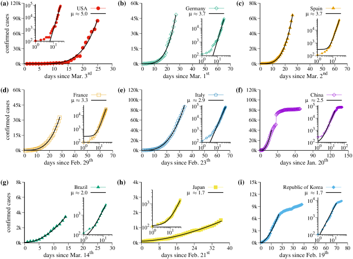
The most desired behavior is that the exponent becomes smaller leading to a flattening of the curves. But this is apparently not that easy. Besides USA and Germany, which have a distinct inclination in the beginning of their power-laws, and China and Republic of Korea, which are stabilizing the epidemic spread, for all other countries the growth remains strictly on the fitted curve and essentially does not change in time. In Sec. III we discuss some possibilities to flatten the power-laws.
II.2 Distance Correlation between countries
The power-law observed in all cases from Fig. 1 are certainly not a coincidence, but a consequence of virus propagation in scale free systems. To quantify the relation between the power-law growth we use the DC, which is a statistical measure of dependence between random vectors Székely et al. (2007); Székely and Rizzo (2009, 2012, 2013, 2014). Please do not confuse the word distance with the geographical distance between the analyzed countries. The most relevant characteristics of DC is that it will be zero if and only if the data are independent and equal to one for maximal correlation between data. Details about the definition of DC are given in Appendix A.
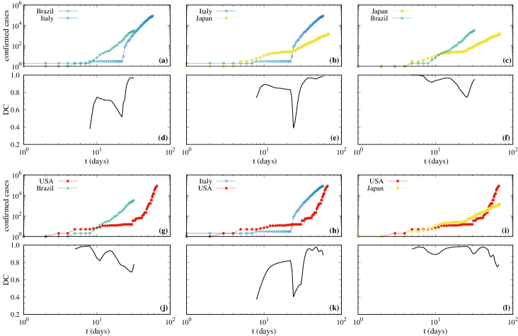
Figure 2 presents specific results for the DC calculated between some selected countries, namely Brazil, Italy, Japan, and USA. Italy were chosen due to their relevance in Europe, relevance regarding to typical data of the virus. USA was chosen for being nowadays the top affected country and Brazil and Japan representing distinct continents and distinct epidemic containment measures. Thus, we compute the DC between four continents. Figures 2(a), 2(b), 2(c), 2(g), 2(h), and 2(i) are the cumulative number of confirmed cases in each country, as in Fig. 1, but considering data since the first day the infections were reported. In these curves we clearly see the initial plateaus due to the incubation time. After the plateaus, a qualitative change to a power-law growth (the same from Fig. 1) occurs. The time for which the qualitative change occurs is distinct for each country.
Figures 2(d), 2(e), 2(f), 2(j), 2(k), and 2(l) display the corresponding DC calculated between the countries. Results show that DC between the curves is relatively high in the beginning. The lowest values are obtained for the DC between Brazil and Italy, in Fig. 2(d), and for the DC between Italy and USA, shown in Fig. 2(k), both cases around DC . The DC decays substantially when the power-law starts in one country but not in the other. The exception is between Japan and USA. After some days, when both countries reach the power-law behavior, the values of DC become very close to . Thus, they are highly correlated besides distinct exponents . Furthermore, the DC is not necessarily related to the exponent . One example can be mentioned. Even though USA has the largest exponent and Japan the lowest one (considering the error in Table 1), they are highly correlated. Besides that, even though there are not many data available for Brazil, it seems to become more and more correlated with Italy and Japan.
III Predictions and strategies
The model proposed in this work for the numerical prediction and strategies is presented in details in Appendix B. It is a variation of the well known Susceptible-Exposed-Infectious-Recovered (SEIR) epidemic model Li et al. (1999); Wu et al. (2020) to propose efficient strategies which allow the government to increase the flattening of the power-law curves. Our SEIR model takes into account the isolation of infected individuals Khalil et al. (2012); Coburn et al. (2009); Lipsitch et al. (2003); Maier and Brockmann (2020b). In this case, the quarantine means the identification and isolation of infected individuals. The parameters are divided in two categories: (i) those related to the characteristic of the virus spreading, defined a priori from other studies and (ii) those related to adjusting the model to the real data (for more details please see Appendix B). These parameters can change according to social actions and government strategies.
Numerical results of this section take into account possible interferences or strategies from the government of each country, what means that some parameters must be changed after the last day of the real data. For each distinct strategy, we use distinct colors which are then plotted.
The colors of the subtitles represent the application of distinct strategies which leads to distinct scenarios. For a detailed explanation of variables and parameters, please see the Appendix B. The colors used in Fig. 3 for the distinct scenarios are the following (for continuous curves):
Red curves: the tendency which follows from the behavior of the last points of
real data (last values for and ). This is what happens if
we do not change the current scenario on March
28.
Blue curves: reduction of social interactions by using smaller values of
. Dark blue for , medium blue for and light blue
for .
Green curves: reduction of social interaction together with tests to identify
and isolate asymptomatic and mild symptomatic cases.
Here we use and .
Magenta curves: reduction of social interaction together
with tests to identify and isolate asymptomatic and mild symptomatic cases. Here we use
and .
Orange curves: identification and isolation of asymptomatic
and mild symptomatic cases with rate . In this strategy we do not increase
the social distance and use the last value for obtained in the adjustment.
For the dashed curves the configurations are the same inside each color. However, in these curves, the asymptomatic and mild symptomatic identified cases are not accounted for. We notice that without the realization of tests in the population, the asymptomatic individuals would not be computed.
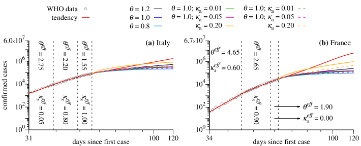
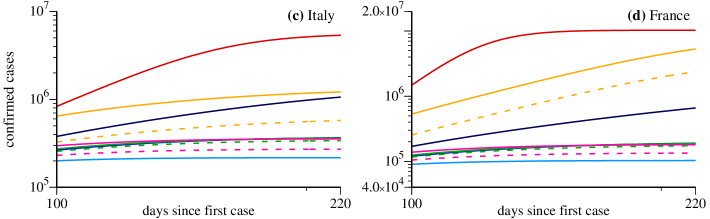
We start discussing the cases of Italy and France, shown in Figs. 3(a), 3(c) and Figs. 3(b), 3(d), respectively. In these cases , which means that we assume that all symptomatic individuals are properly isolated. Figures 3(c) and 3(d) show the evolution of scenarios for . The vertical axis is the cumulative number of positive infected individuals in the population. In the horizontal axis we have the days since the first computed case in these countries. Black circles are the real data starting from the power-law-like behavior discussed in Sec. II. During the times for which real data are available, the model chooses the values of the parameters and that better adjust the simulation results with the data. In the cases shown in Fig. 3 we needed three values of and , namely the values and given in the figures. As a consequence, the red curves are in full agreement with the data in this time interval. When the available data end, the simulation continues and the red curves can be used to predict the asymptotic number of confirmed cases since they represent the scenario following the tendency demonstrated by the data. In the case of Italy we obtain and for France . See the tendencies in Figs. 3(c) and 3(d). The considerable difference between these projections is explained by the last values of and obtained for these countries. Besides being larger for France, we obtain , which can be interpreted as the nonexistence of quarantine measures or the inefficient isolation of symptomatic individuals. We are aware that such asymptotic behavior can be hardly trusted with numerical simulation of models. However, our intention in displaying such asymptotic behavior is to show that the proposed model converges to reasonable values.
Now we discuss results for some emblematic scenarios for the model when specific strategies are applied to Italy and France on day March 28. For both countries we assume for all strategies, which means that all symptomatic individuals per day are putted into quarantine. We can see that the strategy represented by the orange curves is not sufficient to reduce significantly the total number of confirmed infected individuals for France, since the last value indicates a large level of social interaction in this country. On the other hand, for Italy a considerable reduction is observed, specially for the orange-dashed curve, which indicates only the number of symptomatic cases. Strategies related to the blue curves mitigate the growth of the number of confirmed cases and, with exception of the dark blue case for Italy, lead to smaller asymptotic values when compared to the red curves and orange scenarios. The light curves, related to large social distance (), are the most efficient scenarios to induce an accentuated reduction of the growth and a fast convergence to the maximal number of confirmed cases. Furthermore, green curves tend to approach the medium blue curves, which means that, for , there is no significant difference between isolating () of the asymptomatic individuals per day or doing nothing. However, increasing the daily ratio of detection and isolation of asymptomatic individuals to , a noticeable reduction of the asymptotic value of infected individuals is observed (see magenta-dashed curves). Nevertheless, none of these strategies are better than increasing the social distance, scenario represented by the light blue curves.
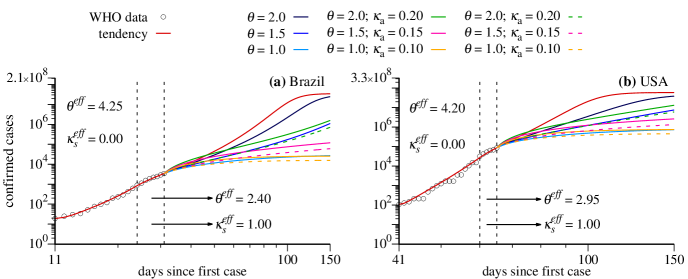
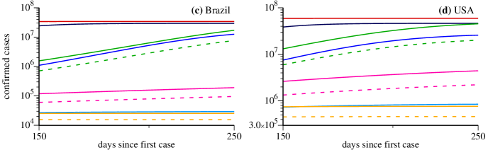
At next we discuss cases for Brazil and USA using other strategies. Results are shown
in Figs. 4(a), 4(c) and Figs. 4(b),
4(d), respectively. Figures 4(c) and 4(d)
furnish predictions for the number of infected individuals. Due to the distinct
scenarios, we had to change a bit the color subtitles (Please see also
color labels in Fig. 4):
Red curves: have the same meaning as before.
Blue curves: are still related to the reduction of social interaction so
that can take the values and , going from dark blue to
light blue.
Green curves: reduction of social interaction together with tests
to identify and isolate asymptomatic and mild symptomatic cases. Here we use
and .
Magenta curves: reduction of social interaction together
with tests to identify and isolate asymptomatic and mild symptomatic cases. Here we use
and .
Orange curves: reduction of social interaction together
with tests to identify and isolate asymptomatic and mild symptomatic cases. Here we use
and .
For the dashed curves, the parameters are the same as those from the continuous
curves above, but represent the total number of confirmed symptomatic individuals. We
notice that asymptomatic individuals, or those with very light symptoms, would not be
identified without realization of tests and are not computed in the number of confirmed
cases.
As in Fig. 3, during the times for which real data are available, the model chooses the values of the parameters and that better adjust the simulation results with the real data. In the case of Brazil and USA we obtain two values of , as shown in Fig. 4(a) and (b) with the corresponding numerical values. Red curves nicely fit the data as long they are available. For the USA case there were some difficult to adjust the parameters since the data show some irregularities. In the case for which the strategy does not change ( and ), the red curves increase very much for both countries. Very high asymptotic values of infected individuals are reached, cases for Brazil and cases for USA.
Now we discuss results when new government strategies are applied to Brazil and USA on March 28. All blue curves (dark to light) tend to mitigate the growth of the asymptotic number of cases for both countries. However, values of and still lead to large asymptotic values. The case with is the most relevant strategy to flatten the curve efficiently. From the strategies which combine social distance with quarantine for the asymptomatic and mild symptomatic cases, stands out the inefficiency of the scenario with and to flatten the green curve. On the other hand, strategies with larger social distance (magenta and orange curves) lead to more promising scenarios. The better prediction emerges when using and (orange curves). For comparison, if we consider only the symptomatic cases, we obtain the asymptotic values (light blue curve) and (orange-dashed curve) for Brazil and (light blue curve) and (orange-dashed curve) for USA. As in the case of France and Italy, also for Brazil and USA we observe that the social distance is the key element to reduce the growth rate of the maximum of symptomatic cases.
IV Conclusions
The power-law growth of the cumulative number of confirmed infected individuals by the COVID-19 until March 27, 2020, is shown to be the best description scenario for the countries: Brazil, China, France, Germany, Italy, Japan, Spain, Republic of Korea, and USA. Distinct power-law exponents for the countries are found and summarized in Table 1. The power-law behavior suggests that the underlying propagation dynamics of the virus around the countries follows scale free networks, fractal kinetics and small world features Watts (2004); Ziff and Ziff (2020); Ray (2020). While power-laws with distinct exponents may look similar visually, it is necessary to quantify this similarity. For this we compute the Distance Correlation Székely et al. (2007); Mendes and Beims (2018); Mendes et al. (2019) between all countries mentioned above (not shown). However, using representative countries of four continents, namely Brazil, Italy, Japan, and USA, results for the DC are presented in Fig. 2. They show that the power-law growth between these countries are highly correlated, even between north and south hemispheres. The high correlation between the power-law curves of different continents strongly suggest that government strategies can be applied with success around the whole World.
Furthermore, we propose a variation of the well known SEIR epidemic model Li et al. (1999); Wu et al. (2020) for predictions using (or not) distinct government strategies applied on March 28, 2020. We apply numerically distinct strategies to flatten (or not) the power-law curves. Even though the social isolation, a well know benefit, is very powerful to flatten the curves, we found other strategies which lead to comparable results. For Italy and France, for example, the best scenario was obtained when reducing the social interaction to (light blue curves). However, if of the asymptomatic and mild symptomatic individuals are identified and isolated every day (), asymptotic values of the same order of magnitude for the symptomatic cases were obtained even if (magenta-dashed curve). On the other hand, for Brazil and USA, our simulations confirm that to keep the social distance is essential to decrease the asymptotic number of infected individuals, and even better results could be obtained by increasing the tests to identify and isolate asymptomatic and mild symptomatic individuals (compare light blue and orange curves). The above combination between social interaction and the huge degree of isolation of infected individuals could be implemented to prevent economic catastrophes because people are not working. In other words, let some essential individuals go back to work (increasing ) and, simultaneously, increase by a huge amount the number of daily tests and isolation of infected individuals. This could furnish an efficient scenario to flatten the power-law.
Nevertheless, we point out again that our main results confirm that the social isolation of individuals is by far the best efficient strategy to flatten the curves.
Appendix A The distance correlation
In this section we give a precise definition of the DC following Székely et al. (2007). Consider joint random sample with and , with and . In addition consider the matrix where is the Euclidean norm of the distance between the elements of the sample, and are the arithmetic mean of the rows and columns, respectively, and is the general mean. A similar matrix can be defined using . The terms , , and are similar to those from matrix . From these matrices we compute the empirical distance correlation from
| (A.1) |
where
| (A.2) |
and
| (A.3) |
Appendix B The Model
The proposed model contains six ODEs and is an extension of a model known in the literature Khalil et al. (2012); Coburn et al. (2009); Lipsitch et al. (2003). Many other related models have been proposed with distinct characteristics Maier and Brockmann (2020b); Long et al. (2020); Hethcote et al. (2002); Khalil et al. (2012); Coburn et al. (2009); Lipsitch et al. (2003); Wu et al. (2020). In our case we consider symptomatic and asymptomatic infected individuals ( also includes individuals with mild symptoms). Quarantine is also contemplated, respectively. The transition rate from asymptomatic to symptomatic cases is neglected as an first approach. The Ordinary Differential Equations (ODEs) are given by
| (B.1) | ||||
| (B.2) | ||||
| (B.3) | ||||
| (B.4) | ||||
| (B.5) | ||||
| (B.6) |
The dot represents the time derivative and the variables are:
-
•
: total population.
-
•
: individuals susceptible to infection.
-
•
: exposed individuals, remain latent until infected.
-
•
: symptomatic individuals. Represent individuals with strong symptoms. We assume that these individuals look for health care and are included in the confirmed cases.
-
•
: asymptomatic individuals and mild symptomatic cases.
-
•
: infected individuals isolated (in quarantine),
-
•
: individuals which were infected and not identified but became immune.
To adjust the parameters following distinct countries, as well as government measures, we used the cumulative number of confirmed infected individuals .The number of confirmed infected individuals as a function of time is defined by . Parameters which do not depend on strategies are:
-
•
days: mean serial interval Li et al. (2020). Is the mean time between successive cases of the transmission of the disease.
- •
-
•
: infectious period Wu et al. (2020).
-
•
: ratio between infectiousness of asymptomatic and symptomatic individuals. We assume that the numbers of asymptomatic and symptomatic individuals are equal.
-
•
: population ratio which remains asymptomatic or mild symptomatic, which is the most common observed cases (see the situation report in Ref. Organization (2020)).
Parameters which are related to the use of distinct strategies are:
-
•
: replication factor, with being a number that represents the proportion of interaction between individuals and the basic reproduction number. In our model, is an adjustable parameter according to WHO data.
-
•
: isolation rate of symptomatic individuals.
-
•
: isolation and identification rate of asymptomatic individuals.
In this model, no rigid quarantine is taken into account and no immunization term is defined, since until today no vaccine has been developed. In Eq. (B.5), the factor dividing represents a rate of exit from the quarantine (for the group ).
It is of most relevance to mention that the only adjustable parameters in our simulations are and . This is important since for systems composed of differential equations with parameters, experiments are need to obtain all the information that is potentially available about the parameters Sontag (2002). Since in our case , we need real data to adjusted parameters correctly. All real data used in Figs. 3 and 4 to find and are larger than . Furthermore, the initial condition for the variable is adjusted only in the first part of the data, where the first and are determined along the data. It could be thought that such initial condition must be include in the adjustable parameters. However, even in such case, and . The lowest number of available data in the first part of data is , as can be seen in Fig. 3(b), meaning that even in the worst case our adjustments are trustful. The goal is to minimize the mean square error between the predicted curve and real data. In the case analyzed here, along the real data. It is only changed, not adjusted, when there are information available about the test realization in the population. We do not start the parameter’s adjustment from the first day of reported infections, but later on. The model produces better results in such cases.
Regarding the adjustment of the parameters , we minimize the mean square error separately inside the three set of data in Figs. 3(a) and 3(b), and inside the two set of data in Figs. 4(a) and 4(b). To do so we vary the parameters inside the intervals and with a step . The initial condition for is determined inside the first part of the data considering in the interval using a step equal .
The initial condition set used in the numerical integration process of the ODEs is the following: ; , where represent the number of confirmed infected cases, obtained from the real time-series for the day . is determined accordingly to the total number of people for each country and the previous initial conditions.
Acknowledgements.
The authors thank CNPq (Brazil) for financial support (grant numbers 432029/2016-8, 304918/2017-2, 310792/2018-5 and 424803/2018-6) and, they also acknowledge computational support from Prof. C. M. de Carvalho at LFTC-DFis-UFPR (Brazil). C. M. also thanks FAPESC (Brazilian agency) for financial support and Luiz A. F. Coelho and Joel M. Crichigno Filho for fruitful discussions.Data availability
The data that support the findings of this study are openly available in WHO (World Health Organization), situation reports 1–68 Organization (2020).
References
- Puevo (2020) T. Puevo, “Coronavirus: Why you must act now,” https://medium.com/@tomaspueyo/coronavirus-act-today-or-people-will-die-f4d3d9cd99c (2020).
- Vazquez (2006) A. Vazquez, “Polynomial growth in branching processes with diverging reproductive number,” Phys. Rev. E 96, 038702 (2006).
- Hethcote (2000) H. W. Hethcote, “The mathematics of infectious diseases,” SIAM Review 42, 599–653 (2000).
- Viswanathan et al. (2011) G. M. Viswanathan, M. G. E. da Luz, E. P. Raposo, and H. E. Stanley, The physics of foraging: an introduction to random searches and biological encounters (Cambridge University Press, 2011).
- Watts (2004) D. J. Watts, Small worlds: the dynamics of networks between order and randomness (Princeton University Press, 2004).
- Ray (2020) T. Ray, “Graph theory suggests COVID-19 might be a ‘small world’ after all,” https://www.zdnet.com/article/graph-theory-suggests-covid-19-might-be-a-small-world-after-all/ (2020).
- Singer (2020) H. M. Singer, “Short-term predictions of country-specific COVID-19 infection rates based on power law scaling exponents,” arXiv:2003.11997v1 (2020).
- Maier and Brockmann (2020a) B. F. Maier and D. Brockmann, “Effective containment explains sub-exponential growth in confirmed cases of recent COVID-19 outbreak in Mainland China,” arXiv:2002.07572v1 (2020a).
- Ziff and Ziff (2020) A. Ziff and R. Ziff, “Fractal kinetics of COVID-19 pandemic,” https://doi.org/10.1101/2020.02.16.20023820 (2020).
- Székely et al. (2007) G. J. Székely, M. L. Rizzo, and N. K. Bakirov, “Measuring and testing dependence by correlation of distances,” Ann. Statist. 35, 2769–2794 (2007).
- Mendes and Beims (2018) C. F. O. Mendes and M. W. Beims, “Distance correlation detecting Lyapunov instabilities, noise-induced escape times and mixing,” Physica A 512, 721 – 730 (2018).
- Mendes et al. (2019) C. F. O. Mendes, R. M. da Silva, and M. W. Beims, “Decay of the distance autocorrelation and Lyapunov exponents,” Phys. Rev. E 99, 062206 (2019).
- Organization (2020) World Health Organization, “Coronavirus disease (COVID-2019) situation reports,” https://www.who.int/emergencies/diseases/novel-coronavirus-2019/situation-reports/ (2020).
- PreventionWeb (2020) PreventionWeb, “How South Korea is suppressing COVID-19,” https://www.preventionweb.net/news/view/71028 (2020).
- Székely and Rizzo (2009) G. J. Székely and M. L. Rizzo, “Brownian distance covariance,” Ann. Appl. Stat. 3, 1236–1265 (2009).
- Székely and Rizzo (2012) G. J. Székely and M. L. Rizzo, “On the uniqueness of distance covariance,” Stat. Probabil. Lett. 82, 2278–2282 (2012).
- Székely and Rizzo (2013) G. J. Székely and M. L. Rizzo, “The distance correlation t-test of independence in high dimension,” J. Multivariate Anal. 117, 193–213 (2013).
- Székely and Rizzo (2014) G. J. Székely and M. L. Rizzo, “Partial distance correlation with methods for dissimilarities,” Ann. Stat. 42, 2382–2412 (2014).
- Li et al. (1999) M. Y. Li, J. R. Graef, L. Wang, and J. Karsai, “Global dynamics of a SEIR model with varying total population size,” Math. Biosci. 160, 191 – 213 (1999).
- Wu et al. (2020) J. T. Wu, K. Leung, and G. M. Leung, “Nowcasting and forecasting the potential domestic and international spread of the 2019-nCoV outbreak originating in Wuhan, China: a modelling study,” The Lancet 395, 689 – 697 (2020).
- Khalil et al. (2012) K. M. Khalil, M. Abdel-Aziz, T. T. Nazmy, and A. B. M. Salem, “An agent-based modeling for pandemic influenza in Egypt,” in Handbook on Decision Making (Springer, 2012) pp. 205–218.
- Coburn et al. (2009) B. J. Coburn, B. G. Wagner, and S. Blower, “Modeling influenza epidemics and pandemics: insights into the future of swine flu (H1N1),” BMC Med. 7, 30 (2009).
- Lipsitch et al. (2003) M. Lipsitch et al., “Transmission dynamics and control of severe acute respiratory syndrome,” Science 300, 1966–1970 (2003).
- Maier and Brockmann (2020b) B. F. Maier and D. Brockmann, “Effective containment explains sub-exponential growth in confirmed cases of recent COVID-19 outbreak in Mainland China,” arXiv preprint arXiv:2002.07572 (2020b).
- Long et al. (2020) Y. S. Long et al., “Quantitative assessment of the role of undocumented infection in the 2019 novel coronavirus (COVID-19) pandemic,” arXiv preprint arXiv:2003.12028 (2020).
- Hethcote et al. (2002) H. Hethcote, M. Zhien, and L. Shengbing, “Effects of quarantine in six endemic models for infectious diseases,” Math. Biosci. 180, 141 – 160 (2002).
- Li et al. (2020) Q. Li et al., “Early transmission dynamics in Wuhan, China, of novel coronavirus–infected pneumonia,” N. Engl. J. Med. 382, 1199–1207 (2020).
- Sontag (2002) E. D. Sontag, “For differential equations with parameters, experiments are enough for identification,” J. Nonlinear Sci. 12, 553 (2002).