LPHYS 2010 contribution 6.5.4 (jacques.tempere@ua.ac.be)]

Strong coupling treatment of the polaronic system consisting of an impurity in a condensate

W. Casteels¹, T. Van Cauteren¹, J. Tempere^1,2 and J. T. Devreese¹ wim.casteels@ua.ac.be ¹TQC, Universiteit Antwerpen, Groenenborgerlaan 171, B2020 Antwerpen, Belgium, ²Lyman Laboratory of Physics, Harvard University, Cambridge, Massachusetts 02138, USA.

([)

Abstract

The strong coupling treatment of the Fröhlich-type polaronic system, based on a canonical transformation and a standard Landau-Pekar type variational wave function, is applied to the polaronic system consisting of an impurity in a condensate. Within this approach the Relaxed Excited States are retrieved as a typical polaronic feature in the energy spectrum. For these states we calculate the corresponding effective mass and the minimal coupling constant required for them to occur. The present approach allows to derive approximate expressions for the transition energies between different Relaxed Excited States in a much simpler way than with the full Mori-Zwanzig approach, and with a good accuracy, which improves with increasing coupling. The transition energies obtained here can be used as the spectroscopic fingerprint for the experimental observation of Relaxed Excited States of impurities in a condensate.

Other Bose-Einstein condensation phenomena

pacs:

03.75.Hh, 03.75.Hh, 71.38.Fp

I Introduction

Ultracold gasses have shown to be very useful for experimentally testing predictions from many-body theories that arose in the context of condensed matter physics. Their study has proven to be especially adequate for strong coupling regimes or when there is strong correlation RevModPhys.80.885 . Recently it has been demonstrated that if the Bogoliubov approximation is valid the system existing of an impurity in a Bose-Einstein condensate (BEC) can be appended to this list by a mapping to the Fröhlich polaron system PhysRevLett.96.210401 , PhysRevA.73.063604 . The Fröhlich polaron, originally introduced in condensed matter physics, is a quasi-particle consisting of an electron with its self-induced polarization cloud. The Fröhlich polaron Hamiltonian has resisted exact analytical diagonalization and has been submitted to many approximation methods (for a detailed review of the Fröhlich polaron in condensed mater physics we refer to Ref. Polarons and for more specialized topics to Ref. BoekDevreese ). The most successful of these methods is the variational path integral approach developed by Feynman in Ref. PhysRev.97.660 . A polaronic coupling parameter was identified that allows to make a distinction between three regimes: weak coupling, intermediate coupling and strong coupling. Also the internal excitation structure of the polaron was investigated by studying the optical absorption and in the intermediate and strong coupling regime a resonance was found PhysRevLett.22.94 , PhysRevB.5.2367 . This resonance was associated with a transition to a Relaxed Excited State (RES), an excitation in which the induced lattice polarization is (self-consistently) adapted to the excited state of the electron. More recently the polaron optical absorption was studied numerically with diagrammatic quantum Monte Carlo numerical techniques PhysRevLett.91.236401 . At strong coupling some differences in the linewidth were found between the spectra derived in PhysRevB.5.2367 and PhysRevLett.91.236401 . Recently these differences were better understood through the introduction of the Extended Memory Function Formalism (see Ref. PhysRevLett.96.136405 ) but they have not yet been completely clarified. Also no material is known that exhibits polaronic strong coupling. A better understanding of the intermediate and strong coupling regimes is needed, i.a. since polaronic effects may play an important role in unconventional pairing mechanisms occurring in high-temperature superconductivity SupercondBipolarons .

In the present work we start by recalling the polaronic system consisting of an impurity in a BEC and some standard results from the strong coupling approximation. Subsequently, the standard strong coupling approximation is applied to the system consisting of an impurity in a BEC. Within this approximation a study is presented of the Relaxed Excited States and the internal transition frequencies of the BEC-impurity polaron. These results are compared with the more detailed study of the internal excitation spectrum of Ref. Bragg . Furthermore the minimal coupling parameters required for the Relaxed Excited States to appear are deduced, and the effective masses corresponding to these states are obtained.

I.1 The polaronic system consisting of an impurity in a condensate

In Ref. PhysRevB.80.184504 it is shown that if the Bogoliubov approximation is valid the Hamiltonian of an impurity in a condensate can be written as the sum of a mean field term and the Fröhlich polaron Hamiltonian $\hat{H}_{pol}$ , given by:

\widehat{H}_{pol}=\frac{\widehat{p}^{2}}{2m_{I}}+\sum_{\vec{k}}\hbar\omega_{\vec{k}}\widehat{a}_{\vec{k}}^{{\dagger}}\widehat{a}_{\vec{k}}+\sum_{\vec{k}}V_{\vec{k}}e^{i\vec{k}.\widehat{\vec{r}}}\left(\widehat{a}_{\vec{k}}+\widehat{a}_{-\vec{k}}^{{\dagger}}\right).

(1)

In this expression the first term represents the kinetic energy of the impurity with mass $m_{I}$ and position (momentum) operators $\widehat{r}$ ( $\widehat{p}$ ), the second term is the kinetic energy of the Bogoliubov excitations with creation (annihilation) operator $\widehat{a}_{\vec{k}}^{{\dagger}}$ ( $\widehat{a}_{\vec{k}})$ and the third term describes the interaction between the impurity and the Bogoliubov excitations. The Bogoliubov dispersion is given by:

\hbar\omega_{\vec{k}}=ck\sqrt{1+\left(\xi k\right)^{2}/2},

(2)

where use was made of the healing length of the condensate: $\xi=1/\sqrt{8\pi a_{BB}n_{0}}$ and the speed of sound in the condensate: $c=\hbar/\left(\sqrt{2}m_{B}\xi\right)$ , with $n_{0}=N_{0}/V$ the condensate density, $a_{BB}$ the boson-boson scattering length and $m_{B}$ the mass of the bosons. The interaction amplitude is given by:

V_{\vec{k}}=\sqrt{N_{0}}\left[\frac{\left(\xi k\right)^{2}}{\left(\xi k\right)^{2}+2}\right]^{1/4}g_{IB},

(3)

where $g_{IB}$ is the amplitude of the impurity-boson contact potential which (at low temperature) is completely determined by the relative mass $m_{r}$ and the impurity-boson scattering length $a_{IB}$ through $g_{IB}=2\pi\hbar^{2}a_{IB}/m_{r}$ . The Feynman variational path integral technique was applied to this specific polaron system in Ref. PhysRevB.80.184504 and it appeared that in this case the polaronic coupling parameter $\alpha$ can be defined as follows:

\alpha=\frac{a_{IB}^{2}}{a_{BB}\xi}.

(4)

As in the case of the solid-state Fröhlich polaron a transition was found between a weak coupling regime and a strong coupling regime. Furthermore it was noted that the polaronic coupling parameter (4) can be tuned externally by a magnetic field through a Feshbach resonance (see e.g. Pitaevskii ). With this technique a coupling parameter $\alpha$ of the order of $10$ is expected to be experimentally feasible. This suggests that by examining an impurity in a condensate it may be possible to experimentally reveal the internal excitation structure of the polaronic strong coupling regime for the first time.

I.2 Standard polaron strong coupling treatment

In this section a summary of the polaronic strong coupling approximation is presented which was introduced by Landau and Pekar for the description of the ground state in Ref. LandauPekar . These results were shown to be accurate in the asymptotic strong coupling limit for a symmetrical, exactly soluble one dimensional polaron model in Ref. Devreese1966196 . The strong coupling formalism was later extended for the calculation of the energy level of the lowest Relaxed Excited State in Refs. Pekar ; Bogoliubov .

The product Ansatz is assumed which means that the wave function of the system $\left|\Psi\right\rangle$ can be written as the product of the wave functions of the impurity $\left|\psi_{I}\right\rangle$ and the Bogoliubov excitations $\left|\phi\right\rangle$ : $\left|\Psi\right\rangle=\left|\psi_{I}\right\rangle\left|\phi\right\rangle$ . The wave function $\left|\phi\right\rangle$ is assumed to be of the form: $\left|\phi\right\rangle=\hat{U}\left|0\right\rangle$ , with $\left|0\right\rangle$ the vacuum and $\hat{U}$ a canonical transformation:

\hat{U}=\exp\left[\sum_{\vec{k}}\left(f_{\vec{k}}\widehat{a}_{\vec{k}}-f_{\vec{k}}^{\ast}\widehat{a}_{\vec{k}}^{{\dagger}}\right)\right],

(5)

with $\left\{f_{\vec{q}}\right\}$ variational parameters. If the expectation value of the polaron Hamiltonian with respect to $\left|\Psi\right\rangle$ is minimized as a function of the variational functions $\left\{f_{\vec{q}}\right\}$ the following standard expression is found for the energy:

E=K-\sum_{\vec{k}}\frac{\left|V_{\vec{k}}\right|^{2}\left|\rho_{\vec{k}}\right|^{2}}{\hbar\omega_{\vec{k}}}.

(6)

where the kinetic energy $K$ and the Fourier transform of the density $\rho_{\vec{k}}$ of the impurity were introduced:

	$\displaystyle K$	$\displaystyle=\left\langle\psi_{I}\left\|\frac{\widehat{p}^{2}}{2m_{I}}\right\|\psi_{I}\right\rangle;$		(7)
	$\displaystyle\rho_{\vec{k}}$	$\displaystyle=\left\langle\psi_{I}\left\|e^{i\vec{k}.\widehat{\vec{r}}}\right\|\psi_{I}\right\rangle.$		(8)

Expression (6) is strictly speaking an upper bound for the groud state energy. When considering excitations of the impurity’s wave function, it is assumed that expression (6), with appropriate $\rho_{\vec{k}}$ , gives a good approximation for the energy of the excited polaron.

I.3 Effective mass

The above formalism can be extended to allow for a calculation of the strong-coupling polaron effective mass Pekar ; Bogoliubov ; Vansant ; Evrard1965295 . The total momentum $\mathcal{\vec{P}}$ of the polaron system, given by $\mathcal{\vec{P}=}\widehat{\vec{p}}+\sum_{\vec{k}}\hbar\vec{k}\widehat{a}_{\vec{k}}^{{\dagger}}\widehat{a}_{\vec{k}}$ , commutes with the polaron Hamiltonian (1) and is conserved. After introducing a Lagrange multiplier $\vec{v}$ the following expression has to be minimized:

\widehat{H}\left(\vec{v}\right)=\widehat{H}_{pol}-\vec{v}.\left(\widehat{\vec{p}}+\sum_{\vec{k}}\hbar\vec{k}\widehat{a}_{\vec{k}}^{{\dagger}}\widehat{a}_{\vec{k}}-\mathcal{\vec{P}}\right),

(9)

with $\vec{v}$ a Lagrange multiplier which physically corresponds to the averaged velocity of the polaron. The polaron effective mass $m^{\ast}$ is then determined from the relation between the momentum and the averaged velocity of the polaron: $\mathcal{\vec{P}}=m^{\ast}\vec{v}$ . The trial wave function for a system in which the polaron moves with velocity $\vec{v}$ is, i.e.:

\left|\Psi\right\rangle=\exp\left[\frac{im_{I}\vec{v}.\widehat{\vec{r}}}{\hbar}\right]\left|\psi_{I}\right\rangle\left|\phi\right\rangle,

(10)

If the expectation value of $\widehat{H}\left(\vec{v}\right)$ is taken with respect to $|\Psi>$ and then minimized as a function of the variational functions $\left\{f_{\vec{q}}\right\}$ the following expression is found for the energy:

E\left(\vec{v}\right)=K-\frac{m_{I}v^{2}}{2}+\vec{v}.\mathcal{\vec{P}}-\sum_{\vec{k}}\frac{\left|V_{\vec{k}}\right|^{2}\left|\rho_{\vec{k}}\right|^{2}}{\hbar\omega_{\vec{k}}-\hbar\vec{v}.\vec{k}}.

(11)

The next step is the minimization with respect to the Lagrange multiplier $\vec{v}$ . If a Taylor expansion is performed for small $\vec{v}$ an expression is found for the effective mass:

m_{ij}^{\ast}=m_{I}+2\hbar^{2}\sum_{\vec{k}}\frac{\left|V_{\vec{k}}\right|^{2}\left|\rho_{\vec{k}}\right|^{2}}{\left(\hbar\omega_{\vec{k}}\right)^{3}}k_{i}k_{j},

(12)

with $i,j=x,y,z$ . Expression (12) results in an anisotropic effective mass for a general density $\rho_{\vec{k}}$ . Since there are no preferred directions in the system, the physically realized effective mass is the lowest eigenvalue of the tensor $m_{ij}^{\ast}$ , since it results in the lowest energy.

I.4 Variational wave function for the impurity

In the present strong coupling approximation it is assumed that the impurity is localized. The self-induced potential is approximated as quadratic which means that the impurity wave function is chosen to be an eigenstate of the harmonic oscillator:

\psi_{n_{x},n_{y},n_{z}}\left(\lambda,\vec{r}\right)=\prod_{i=x,y,z}\left(2^{n_{i}}n_{i}!\right)^{-1/2}\frac{1}{\pi^{1/4}\lambda^{1/2}}H_{n_{i}}\left(\frac{i}{\lambda}\right)\exp\left(-\frac{r^{2}}{2\lambda^{2}}\right),

(13)

with $H_{n_{i}}$ the Hermite polynomials, $n_{i}=0,1,2,...$ and $\lambda$ the oscillator length which is taken as a variational parameter. Physically the oscillator length $\lambda$ can be understood as a measure of the extension of the wave function, a small $\lambda$ corresponding to a small wave function and thus a highly localized state. The kinetic energy (7) is given by:

K_{n}\left(\lambda\right)=\frac{1}{2}\left(\frac{3}{2}+n\right)\frac{\hbar^{2}}{m_{I}\lambda^{2}},

(14)

with $n=n_{x}+n_{y}+n_{z}$ . The Fourier transform of the density (8) can also be calculated as a function of $\lambda$ and $\vec{k}$ and it turns out to be a function of $\vec{q}=\lambda\vec{k}$ , i.e. $\rho_{\vec{k}}\left(\lambda\right)=\rho\left(\vec{q}\right)$ .

II Strong coupling approximation applied to an impurity in a condensate

In this section we introduce the Bogoliubov dispersion (2) and the interaction amplitude (3) for the polaronic system consisting of an impurity in a condensate. If the impurity wave function is assumed to be a harmonic oscillator eigenstate (13) the following expression is found for the energy (6) (with polaronic units, i.e. $\hbar=\xi=m_{I}=1$ ):

E\left(\lambda\right)=\frac{1}{2\lambda^{2}}\left(\frac{3}{2}+n\right)-\frac{\alpha\mu}{2\pi^{2}}\int d\vec{k}\frac{\rho_{\vec{k}}^{2}\left(\lambda\right)}{2+k^{2}},

(15)

where $\alpha$ is the polaronic coupling parameter (4) and $\mu$ is given as:

\mu=\frac{\left(1+m_{B}\right)^{2}}{4m_{B}}.

(16)

From (15), it can be seen that the effective coupling parameter is actually a product of $\alpha$ and the mass imbalance $\mu$ between bosonic atoms and the impurity atoms. The effective coupling constant $\alpha\mu$ can be enhanced by choosing strongly unequal masses, making $\mu$ large. In what follows, we study the system properties as a function of $\alpha\mu$ rather than $\alpha$ . Since the density of the harmonic oscillator eigenfunctions is a function of $\lambda\vec{k}$ only, (15) can be rewritten as:

E\left(\lambda\right)=\frac{1}{2\lambda^{2}}\left(\frac{3}{2}+n\right)-\frac{\alpha\mu}{2\pi^{2}\lambda}\int d\vec{q}\frac{\rho^{2}\left(\vec{q}\right)}{2\lambda^{2}+q^{2}}.

(17)

Minimization of (17) results in the following condition on the variational parameter $\lambda$ :

\frac{1}{\lambda^{3}}\left(\frac{3}{2}+n\right)=\frac{2\alpha\mu}{\pi^{2}}\left(\int d\vec{q}\frac{\rho^{2}\left(\vec{q}\right)}{\left(2\lambda^{2}+q^{2}\right)^{2}}+\frac{1}{4\lambda^{2}}\int d\vec{q}\frac{\rho^{2}\left(\vec{q}\right)}{2\lambda^{2}+q^{2}}\right).

(18)

This equation determines a minimal value for $\alpha\mu$ below which no solution is found, i.e. the requirement to find a solution is:

\alpha\mu\geq\min_{\lambda\in\mathcal{R}^{+}}\left[\frac{\pi^{2}\left(n+3/2\right)}{2\lambda^{3}\left(\int d\vec{q}\frac{\rho^{2}\left(\vec{q}\right)}{\left(2\lambda^{2}+q^{2}\right)^{2}}+\frac{1}{4\lambda^{2}}\int d\vec{q}\frac{\rho^{2}\left(\vec{q}\right)}{2\lambda^{2}+q^{2}}\right)}\right].

(19)

Values of $\alpha\mu$ not satisfying (19) would give $\lambda\rightarrow\infty$ and thus a completely delocalized impurity meaning that the self-induced trapping potential is too shallow to have this type of wave function as a bound state. For the ground state this behavior was already observed in Ref. PhysRevB.80.184504 where above a critical $\alpha$ a state with a large effective mass and a localized impurity wave function was found.

Introducing the Bogoliubov dispersion (2) and the interaction amplitude (3) in the effective mass (12) results in (in polaronic units):

m_{ij}^{\ast}=1+\frac{4\alpha\mu m_{B}^{2}\lambda}{\pi^{2}}\int d\vec{q}\frac{\rho^{2}\left(\vec{q}\right)}{\left(2\lambda^{2}+q^{2}\right)^{2}}\dfrac{q_{i}q_{j}}{q^{2}}.

(20)

III Relaxed Excited States

If an excited state wave function is considered for the impurity, the resulting polaronic state is a Relaxed Excited State (RES). This corresponds to an excitation of the impurity in the self-induced potential adapted to the excited state’s wave function. In this section the numerical solutions for the strong-coupling approach are examined for the ground state and the three lowest Relaxed Excited States. Polaronic units are used, i.e. $\hbar=m_{I}=\xi=1$ .

For the ground state, $n=0$ has to be considered. The first RES corresponds to $n=1$ , i.e. one of the $n_{i}$ ’s is taken to be $1$ . The second RES, corresponding to $n=2$ , can be realized in two distinct ways: either one $n_{i}$ equals $2$ or two $n_{i}$ ’s equal $1$ which will be indicated as $2a$ and $2b$ , respectively.

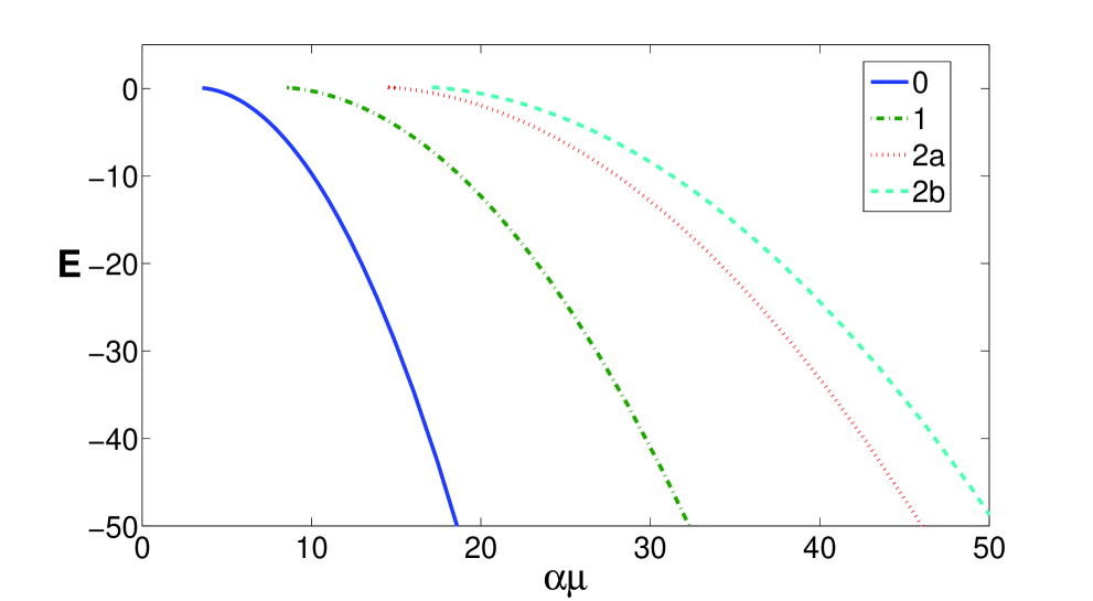
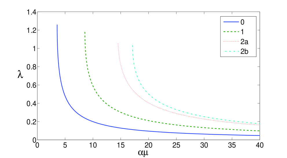
Refer to caption — Figure 1: The variationally determined energy levels in the self-induced potential as a function of the coupling parameter $\alpha\mu$ for the ground state (” $0$ ”), for the first Relaxed Excited State (” $1$ ”) and for the two types of second Relaxed Excited States (” $2a$ ” and ” $2b$ ”).

In figure 1 the variationally determined energy levels are shown as a function of $\alpha\mu$ for all states discussed above and in figure 2 the variational optimal oscillator length of the impurity is shown. Note that the energies of the excited states possess no variational upper bound character. To the left of the curves, the coupling $\alpha\mu$ is too weak for the self-induced potential to support these levels. For couplings just large enough for the level to exist, it is metastable. There are, for each state, two special values of $\alpha\mu$ : one at which the self-induced potential allows for that state to exist, and one at which the polaron energy (6) becomes negative, leading to a stable state. We list these values together with the corresponding optimal value of the variational parameter $\lambda$ in table 1. From figure 2 it is clear that an increase of $\alpha\mu$ results in a decrease of $\lambda$ , corresponding to a stronger self-induced potential and thus to a more localized impurity within the polaron. Furthermore we see that at a given $\alpha\mu$ different oscillator lengths are found for different states which means that not only the wave function of the BEC relaxes but also the impurity’s wave function is adapted.

	$\left(\alpha\mu\right)_{exist}$	$\ \ \ \lambda$	$(\alpha\mu)_{stable}$	$\ \ \ \lambda$
ground state	$3.56641$	$1.2668$	$3.83302$	$0.8213$
first RES	$8.55492$	$1.1850$	$9.10277$	$0.7646$
second RES (2a)	$14.4869$	$1.1495$	$15.3764$	$0.7400$
second RES (2b)	$17.1152$	$1.0570$	$18.0197$	$0.6852$

Table 1: The values of

\alpha\mu

above which the self-induced potential supports the indicated levels is given, along with the corresponding values of the variational parameter

\lambda

(cf. eq. (19)). The last two columns give the values of

\alpha\mu

(and the corresponding

\lambda

) above which the indicated levels become stable.

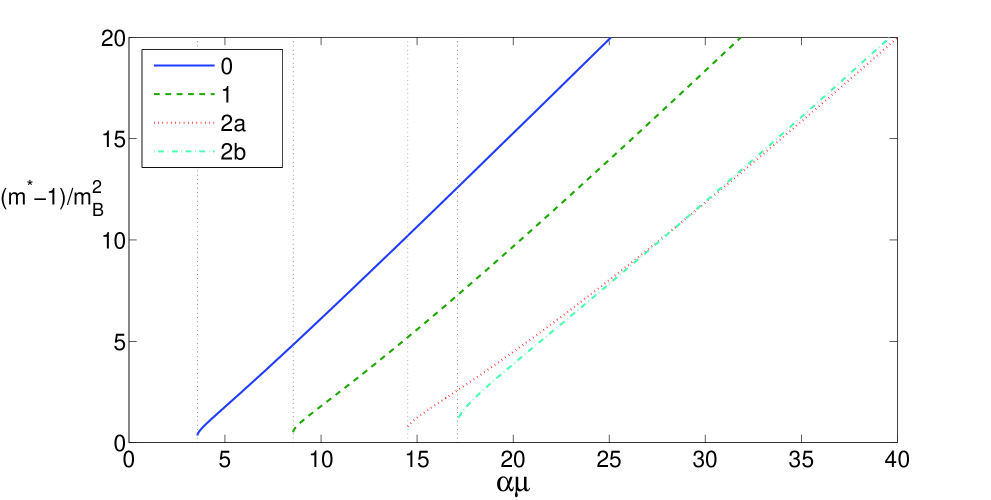
In figure 3, $(m^{\ast}-1)/m_{B}^{2}$ is shown, where $m^{\ast}$ is the effective mass for the states under consideration. The largest effective mass is found for the ground state and it is observed that the effective masses corresponding to the two possibilities for the second RES cross at a coupling parameter $\alpha\mu\approx 28.7$ .

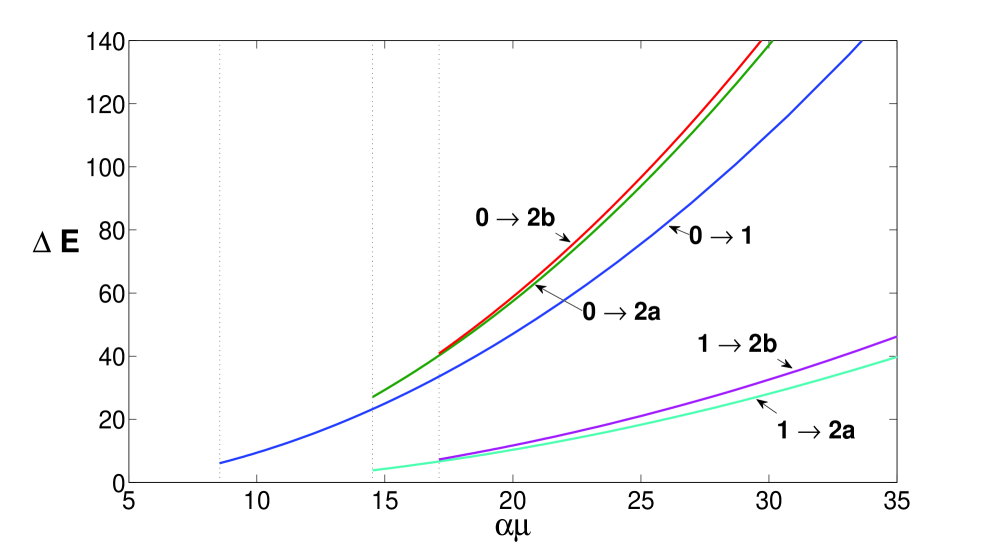
In figure 4 the transition energies are shown for the transition from the ground state to the Relaxed Excites States under consideration and from the first RES to the two types of the second RES. For larger $\alpha\mu$ more Relaxed Excited States are expected to exist and as a result there will be more possible transition energies.

Recently a more detailed study of the excitation structure of the polaron system consisting of an impurity in a condensate was performed by calculating the response of the system to Bragg spectroscopy within the Mori-Zwanzig projection operator formalism Bragg . In this case the system consisting of a lithium impurity in a sodium condensate was examined which results for the present treatment in $\mu=1.5209$ for the mass parameter (16). With this value of $\mu$ the present theory is able to describe the strong coupling ground state from $\alpha\gtrapprox 2.5$ . The self-induced potential becomes deep enough to support a first Relaxed Excited State at $\alpha\approx 6$ . In Ref. Bragg the transition to the first Relaxed Excited State is already seen at $\alpha=4$ and for larger $\alpha$ a larger transition frequency is found, a behavior which is also observed in figure 4. This shows that the lowest $\alpha$ at which the Relaxed Excited State appears is slightly smaller in the treatment of Ref. Bragg and somewhat larger in the present strong coupling treatment. A comparison of the transition frequency from the ground state to the first Relaxed Excited State can be made for $\alpha$ larger than $6$ . At $\alpha=8$ this results in a difference of about $10\%$ and at $\alpha=10$ a deviation of about $5\%$ is found. This trend of a better correspondence between the present strong coupling approximation and the arbitrary coupling treatment of Ref. Bragg at higher coupling parameter is consistent since the present strong coupling theory is expected to be more accurate at larger $\alpha$ .

In the present strong coupling calculation the effect of the mass imbalance is contained solely in the factor $\mu$ which grows as the masses differ more, leading to a larger $\alpha\mu$ . This observation provides an additional tool for facilitating the probing of the strong coupling regime, namely choosing the masses as different as possible: a lithium impurity in a rubidium condensate will correspond to a more strongly interacting system at the same (Feshbach adapted) scattering lengths than a lithium impurity in a sodium condensate.

IV Conclusions

In this work the standard strong coupling approach to polaron theory is applied to investigate the strong coupling regime of the polaronic system consisting of an impurity in a Bose-Einstein condensate. Within this formalism the critical coupling parameters required for Relaxed Excited States to appear were deduced, and the effective masses of these states were calculated. For impurity atoms in a condensate, these states can be experimentally most easily probed by laser spectroscopy. The calculation of the transition energies between different Relaxed Excited States presented here offers a straightforward way to estimate the excitation spectrum. Comparison with the path-integral results for the spectral density obtained within the Mori-Zwanzig framework (see Ref. Bragg ) shows that the current method quickly becomes very accurate ( $<$ 5% for $\alpha\gtrsim 10$ ) as the coupling strength grows. Furthermore it was shown that the polaronic strong coupling regime is easier to reach when the masses of the bosons and the impurity differ more from each other.

References

(1) I. Bloch, J. Dalibard, W. Zwerger, Rev. Mod. Phys. 80, 885 (2008) .
(2) F. M. Cucchietti, E. Timmermans, Phys. Rev. Lett. 96, 210401 (2006).
(3) K. Sacha, E. Timmermans, Phys. Rev. A 73, 063604 (2006).
(4) J. T. Devreese, Polarons, arXiv:cond-mat/0004497v2.
(5) J. T. Devreese, A. S. Alexandrov, Advances In Polaron Physics, (Springer-Verlag Berlin, 2010).
(6) R. P. Feynman, Phys. Rev. 97, 660 (1955).
(7) E. Kartheuser, R. Evrard, J. Devreese, Phys. Rev. Lett. 22, 94 (1969).
(8) J. Devreese, J. De Sitter, M. Goovaerts, Phys. Rev. B 5, 2367 (1972).
(9) A. S. Mishchenko, N. Nagaosa, N. V. Prokof’ev, A. Sakamoto, B. V. Svistunov, Phys. Rev. Lett. 91, 236401 (2003).
(10) G. De Filippis, V. Cataudella, A. S. Mishchenko, C. A. Perroni, J. T. Devreese, Phys. Rev. Lett. 96, 136405.(2006).
(11) A. S. Alexandrov, Polarons in advanced Materials (Springer-Verlag, Berlin, 2007), pp. 257-310 and references therein.
(12) W. Casteels, J. Tempere, J. T. Devreese, submitted to Phys. Rev.
(13) J. Tempere, W. Casteels, M. K. Oberthaler, S. Knoop, E. Timmermans, J. T. Devreese, Phys. Rev. B 80, 184504 (2009).
(14) L. Pitaevskii, S. Stringari, Bose-Einstein Condensation (Oxford University Press, Oxford, 2003).
(15) L. D. Landau, S. I. Pekar, Zh. Eksp. Teor. Fiz. 16, 341 (1946); ibid. 18, 419 (1948).
(16) J. Devreese, R. Evrard, Physics Letters 23, 196 (1966).
(17) S. I. Pekar, Untersuchungen über die elektronentheorie der kristalle, (Akademie Verlag, Berlin, 1951).
(18) N.N. Bogoliubov, Ukrainskij Matematičeskij Žurnal 2, 3 (1950), and in: Advanced in Theoretical Physics, ed. E. Caianiello (World Scientific Publ., Singapore, 1991), p.1-18.
(19) P. Vansant, M.A. Smondyrev, F.M. Peeters, J.T. Devreese, J. Phys. A: Math. Gen. 27, 7925 (1994).
(20) R. Evrard, Physics Letters 14, 295 (1965).