Structure Enhanced Graph Neural Networks for Link Prediction
Abstract.
Graph Neural Networks (GNNs) have shown promising results in various tasks, among which link prediction is an important one. GNN models usually follow a node-centric message passing procedure that aggregates the neighborhood information to the central node recursively. Following this paradigm, features of nodes are passed through edges without caring about where the nodes are located and which role they played. However, the neglected topological information is shown to be valuable for link prediction tasks. In this paper, we propose Structure Enhanced Graph neural network (SEG) for link prediction. SEG introduces the path labeling method to capture surrounding topological information of target nodes and then incorporates the structure into an ordinary GNN model. By jointly training the structure encoder and deep GNN model, SEG fuses topological structures and node features to take full advantage of graph information. Experiments on the OGB link prediction datasets demonstrate that SEG achieves state-of-the-art results among all three public datasets.
1. Introduction
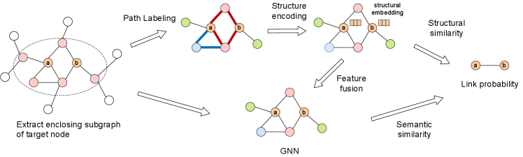
The SEG framework. For target nodes and , SEG first extracts an enclosing subgraph around it, and then extracts paths and jointly trains an encoder and a GNN to learn both graph structure and the original node features for link prediction. Paths are indicated the red and blue bolded edges.
Link prediction, which is used to predict whether two nodes are connected in a graph, is widely applied in various fields, such as recommendation, knowledge graph, and social network. The traditional approaches mainly focus on graph topology. Topology-based methods compute node similarity score as the likelihood of connections, such as Common Neighbors (CN) (Newman, 2001), Jaccard measure (Chowdhury, 2010), Adamic/Adar (AA) measure (Adamic and Adar, 2003), and Katz measure (Katz, 1953). Graph embedding approaches are currently popular to resolve link prediction problems. Representative methods such as DeepWalk (Perozzi et al., 2014), LINE (Tang et al., 2015) and Node2vec (Grover and Leskovec, 2016) are trying to learn parameter-free low-dimensional node embeddings from the observed graph nodes and then use these embeddings to predict links. These approaches potentially belong to transductive learning and therefore cannot predict unseen nodes. Recently, graph neural networks (GNNs) has shown impressive performance on link prediction (Kipf and Welling, 2016; Hamilton et al., 2017; Zhang et al., 2018). GNNs generally follow a message passing schema to aggregate neighborhood vectors recursively and have been proved to be as powerful as the Weisfeiler-Lehman graph isomorphism test (Xu et al., 2019). However, only features of nodes are passed during the message passing procedure, topological information of nodes is not explicitly considered. These topological features are shown to be useful in topology-based methods. Moreover, on some datasets, topology-based methods such as CN are more effective than GNN methods such as GCN (Kipf and Welling, 2016) and GraphSAEG (Hamilton et al., 2017). Based on these observations, scholars began to explicitly extract topological information as an extra input of GNNs (Zhang and Chen, 2018; Li et al., 2020). The SEAL (Zhang and Chen, 2018) method first extracts an enclosing subgraph around the target link and then labels nodes in the subgraph based on their different location. Then a GNN framework named DGCNN (Zhang et al., 2018) is applied to predict the existence of the target link. These works simply use node labeling tricks and directly concatenate structural features with original node features as the input of GNNs. However, which structural features are useful and how to incorporate them with GNNs is still underexplored.
In this work, we attempt to resolve two problems: 1. How to design and encode structural features. 2. How to incorporate structural features into GNNs for link prediction. For the first problem, motivated by topology-based methods, we propose a novel node position labeling method called Path Labeling(PL) to extract nodes’ structural features. Instead of directly using these structural features as the input of a GNN model like SEAL (Zhang and Chen, 2018), we design an encoder to transform structural features to structural embeddings. For the second problem, we propose a novel Structure Enhanced Graph neural network (SEG) to integrate structural embeddings into GNNs. Given structural embeddings mentioned above, SEG uses a feature fusion module to map the structural embeddings and the original node features into the same embedding space. Fused result are then used as the initial input of a GNN model. Through jointly training the structure encoder and GNN, SEG can learn both structure and attribute information of nodes, thus optimizes the usage of graph information for link prediction. The pipeline of SEG is illustrated in Figure 1. To predict the link between two target nodes and , we first extract an enclosing 1-hop subgraph around them. Then we label each node according to their position role in the subgraph to get node structural features, and apply a structure encoder to generate structural embeddings for each node. These structural embeddings are fused with the node features as the input of a GNN model. The output of the GNN model and correlation between structural embeddings of these two target nodes are jointed together to make the final prediction of whether the link exists. Our contributions are summarized as follows:
-
•
We propose a novel node position labeling method called Path Labeling(PL) to encode structural features of graph nodes.
-
•
We propose an end-to-end joint training framework named SEG that learns both structural features and initial node features.
-
•
We validate SEG on three OGB111https://ogb.stanford.edu/docs/linkprop/ link-prediction datasets and achieve the state-of-art result.
The rest of the paper is organized as follows. In Section 2, we will review some related works. Section 3 defines the problem and lists notations we use. We then introduce the proposed method Structure Enhanced Graph neural networks (SEG) in Section 4 and discuss experimental setup and insights in Section 5. Finally, the whole paper is concluded in Section 6.
2. Related Work
In this section, we briefly survey related work in graph neural networks and link prediction.
2.1. Graph Neural Networks
Graphs are ubiquitous in the real world and have a wide range of applications in many fields, including social networks, biological networks, the co-authorship network and the World Wide Web. Over the past few years, Graph Neural Networks (GNNs) have achieved great success on many tasks, including node classification, link prediction, graph classification, and recommender systems(Kipf and Welling, 2016; Hamilton et al., 2017; Zhang and Chen, 2018; Zhang et al., 2018; Ying et al., 2018). GNN uses deep learning methods to solve graph-related problems, which can be seen as an application of deep learning on graph data. One of the most popular methods of GNNs called Graph Convolutional Networks (GCNs). GCNs originated with the work of Bruna et al. (Bruna et al., 2013), which develops a version of graph convolutions based on spectral graph theory. Bruna et al. (Bruna et al., 2013) generalize the convolution operation from Euclidean data to graph data by using the Fourier basis of a given graph. And then Defferrard et al. (Defferrard et al., 2016) propose ChebNet, which utilizes Chebyshev polynomials as the filter to simplify the calculation of the convolution. Kipf et al. (Kipf and Welling, 2016) further simplify ChebNet by using its first-order approximation which is the well-known GCN model. Some approaches define graph convolutions in the spatial domain (Hamilton et al., 2017; Veličković et al., 2017). Hamilton et al. (Hamilton et al., 2017) introduce GraphSAGE which first samples a fixed-sized of neighborhood nodes and then aggregates neighbor information using different strategies. DGCNN (Zhang et al., 2018) proposes a SortPooling layer that sorts graph vertices in a consistent order and then uses a traditional 1-D convolutional neural network for graph classification. Veličković et al. (Veličković et al., 2017) proposes the graph attention network (GAT) model which uses the attention mechanism to assign different weights to different neighborhood nodes when aggregating information.
More recently, there has been a lot of works try to improve the training efficiency of GNNs. FastGCN (Chen et al., 2018) performs layer-wise sampling to solve the neighbor explosion problem of node-wise sampling methods like GraphSAGE (Hamilton et al., 2017). ClusterGCN (Chiang et al., 2019) proposes graph clustering based training method. GraphSAINT (Zeng et al., 2019) proposes the subgraph sampling based training method.
2.2. Link Prediction
Link prediction is a fundamental problem for graph data. It focus on predicting the existence of a link between two target nodes (Liben-Nowell and Kleinberg, 2007). Classical approaches for link prediction are topology-based heuristic methods. Topology-based methods use graph structural features to calculate nodes’ similarity as the likelihood of whether they are connected. Some representative methods include Common Neighbors (CN) (Newman, 2001), Jaccard measure (Chowdhury, 2010), Adamic/Adar (AA) measure (Adamic and Adar, 2003), and Katz measure (Katz, 1953). CN computes the number of common neighbors as similarity scores to predict the link between two nodes. Jaccard measure computes the relative number of neighbors in common. CN and Jaccard only use one-hop neighbors, while the AA method captures two-hop similarities instead. The Katz measure further uses longer paths to capture a larger range of local structures.
Other common approaches are graph embedding methods, which first embed the nodes into low-dimensional space and then calculate the similarity of the nodes’ embeddings to predict the existence of a link. DeepWalk (Perozzi et al., 2014) first generates random walks and then uses Word2vec (Mikolov et al., 2013) to get the embeddings of nodes. LINE (Tang et al., 2015) introduces concepts of first-order and second-order similarity into weighted graphs. Node2vec (Grover and Leskovec, 2016) extend DeepWalk with a more sophisticated random walk strategy that combines the DFS and BFS.
More recently, GNNs (Kipf and Welling, 2016; Hamilton et al., 2017) have been used for link prediction. GNN-based methods typically use supervised learning to model the link prediction as a classification problem. Zhang and Chen (Zhang and Chen, 2017) propose WLNM to extract the enclosing subgraph around the target link and then encode the subgraph as a vector for subsequent classification. Zhang and Chen (Zhang and Chen, 2018) propose SEAL which first labels the nodes in each enclosing subgraph according to their distances to the source and target nodes, and then applies DGCNN (Zhang et al., 2018) to learn a link representation for link prediction. Li et al. (Li et al., 2020) introduces another node labeling trick similar to SEAL which directly uses the shortest distances to target nodes. You et al . (You et al., 2019) propose Position-aware GNN (P-GNN) (You et al., 2019). P-GNN uses anchor nodes to introduce relative location information of nodes into GNNs. The model proposed in this paper also uses the labeling trick introduced in SEAL (Zhang and Chen, 2018). However, SEAL simply concatenates structural features with original features of the nodes as the input of GNNs, which will be improved in this paper.
3. Preliminaries
We consider an undirected graph which can be represented as a graph , where is the set of nodes, is the set of edges, and is the adjacency matrix of the graph, where if and otherwise. A graph can be associated with node features matrix , where and is the dimension of node features.
The goal of link prediction is to determine whether there exists an edge between two given nodes . It can be formulated as a classification problem on potential links given observed edges and observed node features .
General GNN algorithm follows a message passing strategy, where each node’s features can be iteratively updated by aggregating its neighbors’. During each iteration, hidden vector of node is updated by aggregating information from it’s neighborhood . The -th iteration/layer hidden vector of node is calculated as follows:
| (1) |
where is the function of neighborhood aggregation and represents the process of combining the aggregated neighborhood vectors and its own vector . We initialize these embeddings using node features, i.e., . After running iterations, we can get the final layer vector for each node. These vectors can be used in downstream tasks such as node classification and link prediction, etc.
4. APPROACH
In this section, we will detail our Structure Enhanced Graph neural network (SEG) model. Most GNN models treat edges in a graph as message passing routers, while ignoring topological information beneath them. However, topology-based methods, such as AA and CN, make use of structural information directly to successfully predict links.
Inspired by these methods, we propose a novel structure encoding method to extract structural embeddings for each node. To effectively incorporate structural features into GNN, we design the SEG framework to jointly train a deep GNN and a structure encoder.
4.1. Structure Encoding
We first focus on the question that how to design and encode structural features. There are many local structural patterns around target nodes, such as common neighbors and triangles. To measure the correlation between two target nodes, we need to examine the topology of these nodes and edges connect them at the same time. Graph structures like Common Neighbors (CN) (Newman, 2001), Jaccard measure (Chowdhury, 2010), Adamic/Adar (AA) measure (Adamic and Adar, 2003), and Katz measure (Katz, 1953) are shown to be useful for link prediction. These methods can be unified as follows:
| (2) |
where denotes similarity between node and , denotes number of length- paths between target nodes and , and , means neighbor nodes of and , respectively. For example, suppose and , Equation 2 is the same as the Katz measure . If , the equation is the same as neighbor based methods like CN and AA.
Two key components of Equation 2 are paths of target nodes and their neighbor nodes . Since information of neighbors is already considered in GNNs, paths are especially important to be an extra input of GNN models. Here we propose path between two targets nodes as a kind of topological feature, defined as follows:
Definition 4.1 (path).
A path between two target nodes and is a sequence of vertices and undirected edges starting with and ending with in which neither vertices nor edges are repeated.
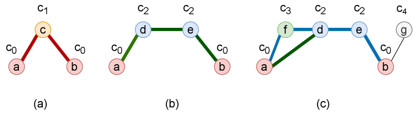
To numericalize these paths as usable topological features for nodes, we propose a Path Labeling(PL) method to label each node with a discrete value based on the path it belongs to. Basically, nodes in different paths of different lengths are labeled with different discrete values. The fringe nodes that are not part of the path are labeled with a default value. For example, all 1-hop fringe nodes have an identical label value. The target nodes are also labeled with a default value. For a node that appears in multiple paths at the same time, we choose the shortest path to label the node.
Figure 2 shows examples of path labeling in the subgraph which consists of 1-hop neighbors of two target nodes and . We label two target nodes and with a discrete value ; The node in (a) is the common neighbor of target nodes, and we label it with ; Nodes and in (b) are located on the path of length 3, we label them with ; Nodes and in (c) are located in both the path of length 3 (a-d-e-b) and length 4 (a-f-d-e-b), so we choose the path of length 3 to label and with value , and label in (c) with . Node is a fringe node, so we label it with a default value .
Given these topological features extracted from paths of each pair of target node, we further propose a structure encoding method to learn representation vectors from them. The encoding method is defined as follows:
Definition 4.2 (Structure Encoding).
Given structural features of node by path labeling method, we design a structure encoder as a mapping , which transform structural features to structural embeddings, where is the dimension of representation vectors of nodes.
This encoding process can be implemented with neural networks. In Algorithm 1, we introduce our structure encoding method. We first extract the paths and then generate structural features for each node according to path labeling(PL). Then we use one-hot method to generate the initial structural embedding of node according to , notes that is first truncated with a constant to prevent too long paths. Finally a GCN layer and a MLP is applied to get the final node structural embeddings.
In Algorithm 1, we use a GCN layer and MLP to fit and in Equation 2. With appropriate parameters and enough layers, we hope the error of approximation can be ignored.
By the way, SEAL (Zhang and Chen, 2018) also uses labeling method to generate structural features. It’s Double-Radius Node Labeling(DRNL) method labels each node according to its radius with respect to the two target nodes. The difference is that DRNL is much more strict than PL, because it distinguishes different nodes in the same length path. For example, given a path (a-b-c-d-e), where and are target nodes, the labeling result of DRNL is (, , , , ) and the result of PL is (, , , , ). In addition, we use a constant to truncate too long paths, these difference prevent PL from overfitting thus more robust than DRNL.
4.2. Feature Fusion
To learn both node attributes and structural information, one straightforward way is to directly concatenate node features and structural features as the input of GNNs like SEAL (Zhang and Chen, 2018). However, these two features express different meanings. The node attributes are usually constructed by semantic information, while the structural features are directly extracted from graph topology. How to learn both semantic information and structural information at the same time is also a challenging problem.
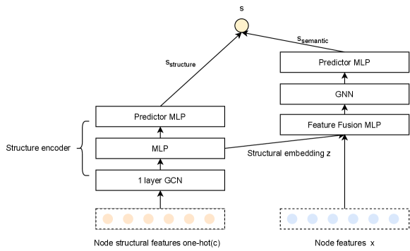
We design a framework to fuse these two features called SEG. The detail architecture is shown in Figure 3. The SEG architecture contains two parts, one is a structure encoder and the other is a deep GNN. In the structure encoder, we start at encoding node structure features () with a single layer GCN. The reason for choosing one layer GCN is that the multi-hop information is already included in the path, so only one layer of aggregation is needed to update two target nodes we focus on. The output of the GCN layer are used as the input of a MLP to fit and in Equation 2. We denote the output vectors of MLP as the structural embeddings of . Another MLP is used to predict the structure similarity score based on the Hadamard product of structural embeddings of target nodes and .
| (3) |
For the deep GNN model, structural embedding and original node attributes are firstly fused by a MLP. The module of feature fusion is to map and into the same feature space. With fused features as the input, a deep GNN model can learn from both structural features and original node features. Here we choose a multi-layers GraphSAGE (Hamilton et al., 2017) as our backbone GNN model and use a SortPooling (Zhang et al., 2018) layer to get the final representation output of two targets nodes. Finally, we use a MLP to predict the high-level semantic similarity score, denoted as . We combine the structure similarity score and semantic similarity score as the final link existence probability:
| (4) |
4.3. Training Algorithm
In this section, we introduce the SEG training algorithm. The GNN updating procedure can be formed in Equation 1. However, in practice, considering the efficiency of training, especially for real-world large graphs, we do not perform the above update process directly on the whole graph (Hamilton et al., 2017; Chiang et al., 2019; Zhu et al., 2019). Instead, we extract a -hop enclosing subgraph of two target nodes from the whole graph . A -hop enclosing subgraph is a graph consisting of -hop neighbors of nodes and . Then, we apply structure encoding described in Algorithm 1 on . Finally, two parts of SEG is jointly training using a sigmoid cross entropy loss,
| (5) |
where refers to the probability score that the link is predicted to be true, is the label of the link , and is the number of training edges. Algorithm 2 details how to generate the final predict score. During training, we randomly sample two nodes that are not connected as negative samples.
5. Experiments
In this section, we conduct experiments on real-world datasets to evaluate the effectiveness of SEG. In particular, we attempt to answer the following questions:
-
•
Can SEG outperform existing baselines for link prediction on various benchmark datasets?
-
•
How effective are structure encoding and joint training of SEG for link prediction?
-
•
Is the Path Labeling(PL) more effective than the Double-Radius Node Labeling(DRNL) of SEAL?
5.1. Experimental Setup
| Dataset | #Nodes | #Edges | Feature Dimension |
|---|---|---|---|
| ogbl-ppa | 576,289 | 30,326,273 | 58 |
| ogbl-collab | 235,868 | 1,285,465 | 128 |
| ogbl-citation2 | 2,927,963 | 30,561,187 | 128 |
| Method | ogbl-ppa | ogbl-collab | ogbl-citation2 |
|---|---|---|---|
| Hits@100 | Hits@50 | MRR | |
| MLP | 0.0046 ± 0.0000 | 0.1927 ± 0.0129 | 0.2904 ± 0.0013 |
| CN | 0.2765 ± 0.0000 | 0.5006 ± 0.0000 | 0.5147 ± 0.0000 |
| Node2vec | 0.2226 ± 0.0083 | 0.4888 ± 0.0054 | 0.6141 ± 0.0011 |
| GCN | 0.1867 ± 0.0132 | 0.4475 ± 0.0107 | 0.8474 ± 0.0021 |
| GraphSAGE | 0.1655 ± 0.0240 | 0.4810 ± 0.0081 | 0.8260 ± 0.0036 |
| SEAL | 0.4880 ± 0.0316 | 0.5371 ± 0.0047 | 0.8767 ± 0.0032 |
| DE-GNN | 0.3648 ± 0.0378 | 0.5303 ± 0.0050 | 0.6030 ± 0.0061 |
| SEG | 0.5059 ± 0.0239 | 0.5535 ± 0.0039 | 0.8773 ± 0.0030 |
5.1.1. Datasets.
We test the proposed SEG for link prediction on the Open Graph Benchmark (OGB) (Hu et al., 2020) datasets. OGB datasets are open-sourced large-scale datasets which cover a diverse range of domains, ranging from social networks, biological networks to molecular graphs. OGB provides standard evaluation metrics to fairly compare the performance of each algorithm. We use three link prediction datasets in OGB including ogbl-ppa (Szklarczyk et al., 2019), ogbl-collab (Wang et al., 2020) and ogbl-citation2 (Wang et al., 2020). The ogbl-ppa dataset is an undirected, unweighted protein-protein association graph with 576,289 nodes and 30,326,273 edges. Each node contains a 58-dimensional embedding that indicates the species that the corresponding protein comes from. The ogbl-collab dataset is an undirected graph, representing a collaboration network between authors. It contains 235,868 nodes and 1,285,465 edges. Nodes represent authors and edges indicate the collaboration between authors. Each node contains 128-dimensional features, generated by averaging the word embeddings of authors’ papers. The ogbl-citation2 dataset is a directed citation graph between a subset of papers with 2,927,963 nods and 30,561,187 edges. Nodes represent papers and each edge indicates that one paper cites another. Each node with pre-trained 128-dimensional Word2vec embedding with its title and abstract. The detailed statistics of the datasets are summarized in Table 1.
5.1.2. Baselines.
We compare SEG with representative and state-of-the-art link prediction algorithms, which includes:
-
•
MLP (Pal and Mitra, 1992) is a basic neural network with node features directly as input. MLP is used to verify whether the original node feature is enough to predict links.
-
•
CN (Newman, 2001) is a common approach for link prediction that computes the number of common neighbors between two nodes as the similarity score of a link between the nodes. Nodes with higher scoring are more likely to have a link.
-
•
Node2vec (Grover and Leskovec, 2016) is a classical graph embedding method that encodes nodes into low dimensional vectors. Then a MLP predictor is applied that uses the combination of the original node features and the Node2vec output vectors as input.
-
•
GCN (Kipf and Welling, 2016) is a well-known graph neural network which defines graph convolution via spectral analysis.
-
•
GraphSAGE (Hamilton et al., 2017) is a widely used graph neural network that uses sample and aggregation tricks to support inductive learning for unseen nodes.
- •
-
•
DE-GNN (Li et al., 2020) is a GNN model which uses shortest-path-distances node labeling instead of DRNL in SEAL.
5.1.3. Evaluation Metric.
In this paper, we adopt metrics that include top-K hit rate (Hits@K) and Mean Reciprocal Rank (MRR). Hits@K counts the ratio of positive edges that are ranked at the K-th place or above against all the negative edges. Hits@K is more challenging than well-known AUC because the model needs to rank positive edges above almost all negative edges. MRR computes the reciprocal rank of the true target edge among the 1,000 negative candidates for each source node and then averages over all these source nodes. Both metrics are higher the better.
5.1.4. Settings and Hyperparameters.
We follow the original OGB dataset splitting, the training/validation/testing set is split as follows, for ogbl-ppa is 70/20/10, for ogbl-collab is 92/4/4, and 98/1/1 for ogbl-citation2. GCN and GraphSAGE have 3 layers with 256 hidden dimensions and two fully-connected layers, each contains 256 hidden units that are applied as the predictor of link existence. For SEAL and DE-GNN, the labeled structural features are concatenated with the node features as input of the GNN model which has 3 layers with 32 hidden units. For a fair comparison with SEAL, we also use a 3 layers with 32 hidden units DGCNN as base model in SEG. DE-GNN uses a 3 layers GCN as its base model. DE-GNN, SEAL and SEG use a 2 layers MLP predictor with 128 units to output the probability of link. For structure encoder in SEG, we use a single layer GCN and 3 layers MLP to encode path features and then use another 2 layers MLP to output the link scores. In the training, for ogbl-ppa we use only 5 of the training edges as positive samples, for ogbl-collab we use 10 of the data, and for ogbl-citation2 we use 2 of the data, which is the same as the setting of SEAL. We set to 4 for all the three datasets to prevent overfitting. The negative link (edge consisting of two nodes that are not connected) is sampled randomly from the training set. We report the averaged results over 10 times of running.
| Method | ogbl-collab |
|---|---|
| CN | 0.6137 ± 0.0000 |
| GCN | 0.4714 ± 0.0145 |
| GraphSAGE | 0.5463 ± 0.0112 |
| SEAL | 0.6364 ± 0.0071 |
| DE-GNN | 0.6440 ± 0.0028 |
| SEG | 0.6445 ± 0.0036 |
5.2. Basic Results
We conduct experiments on three public OGB datasets to answer the first question. It is worth mentioning that the SEAL method has achieved the best performance on these three datasets so far. Experimental results on three OGB datasets are reported in Table 2. Results show that the proposed method SEG beats SEAL and achieves the best performance on all three datasets.
On both ogbl-ppa and ogbl-collab datasets, SEG achieves 3 improvement over the SEAL method. The topology-based method CN achieves higher Hits@K than the Node2vec and GNNs which indicates that the structural information is more important than the original node features in these graphs. Besides, the MLP baseline performs extremely poorly on all three datasets, which shows that the attributes of the nodes in these datasets do not accurately reflect the interaction between the nodes.
As a matter of fact, in many real-world graphs, it is difficult to design high-quality semantic features for target tasks. For these graphs, it is better to effectively use the structural information from graph itself.
For larger scale ogbl-citation2, SEG still outperforms all baselines, which shows the effectiveness of the proposed method. DE-GNN, SEAL and SEG achieve a huge improvement over other GNN models on both ogbl-ppa and ogbl-collab, which illustrates the effectiveness of adding structural information to GNNs. Note that validation edges are also allowed to be included in training (Hu et al., 2020). So we conduct experiments to use the validation edges as training as well. The results in Table 3 show that SEG is still better than all other methods.
5.3. Ablation studies
We next attempt to answer the second and third questions raised at the beginning of this section. We first only use structure encoding part in SEG denoted as SEG-SE, and compare the SEG-SE with SEAL-PL which uses path labeling instead of DRNL in SEAL on the ogbl-collab dataset. The result in Table 4 shows that SEG-SE achieves 0.5503 Hits@50, which is better than SEAL-PL. It demonstrates the effectiveness of our structure encoding. We then remove the final predictor MLP and of structure encoding in SEG, denoted as SEG-GNN, and compare it with SEG-SE and SEG. As shown in Table 4, within these three methods, SEG achieves the best results, which illustrates the benefits of joint training. By joint training, structural embedding can better represent the original structural features.
It is worth noting that the result of SEG-GNN is still better than SEAL, which means our structure encoding method is more effective than DRNL of SEAL (Zhang and Chen, 2018).
| Method | ogbl-collab |
|---|---|
| SEAL | 0.5371 ± 0.0047 |
| SEAL-PL | 0.5393 ± 0.0052 |
| SEG-GNN | 0.5465 ± 0.0021 |
| SEG-DRNL | 0.5476 ± 0.0051 |
| SEG-SE | 0.5503 ± 0.0033 |
| SEG | 0.5535 ± 0.0039 |
This also proves our proposition, which is that the structural information and the original node features are in different spaces and cannot be directly and simply concatenated. Instead, we use a feature fusion module to map these two features to the same space.
To further address the difference between our Path Labeling(PL) and DRNL of SEAL, we conduct an experiment that uses SEAL’s DRNL features as the structural features in the SEG framework, denoted as SEG-DRNL in Table 4. The result shows that SEG outperforms SEG-DRNL. In addition, we replace the DRNL in SEAL with PL named SEAL-PL, and compare it with the original SEAL. The result shows that SEAL-PL is better than original SEAL. It means under the same training framework and settings, the PL are more effective than DRNL. Our analysis of the label values reveals that for the 1-hop subgraph, DRNL has a total of 17 different values of node labels, much more than the 4 of PL. This indicates that more label values introduce noise, so we do not distinguish between labels of nodes of the same path and place a limit on the length of the path to further prevent overfitting. Besides, the Hits@50 of SEG-DRNL is higher than Hits@50 of SEAL on ogbl-collab. It also illustrates the effectiveness of our SEG framework.
5.4. Caveats
There is an ogbl-ddi graph (Wishart et al., 2017) in OGB link prediction datasets which is much denser than the other datasets introduced above. The ogbl-ddi dataset is an undirected graph. Each node represents a drug and the edge represents the interaction between drugs. It has 1,334,889 edges but only has 4,267 nodes. The average degree of the nodes in this graph is 500.5 and the density is 14.67, which is much larger than the other three graphs (see statistics of all datasets in Table 5). Nodes in ogbl-ddi do not contain any feature, so we exclude the MLP method in comparison. All learning-based methods use free-parameter node embeddings as the input. In the SEG method, we only use GNN and exclude structure encoder.
| Dataset | Average Node Degree | Density |
|---|---|---|
| ogbl-ppa | 73.7 | 0.018 |
| ogbl-collab | 8.2 | 0.0046 |
| ogbl-citation2 | 20.7 | 0.00036 |
| ogbl-ddi | 500.5 | 14.67 |
| Method | ogbl-ddi |
|---|---|
| CN | 0.1773 ± 0.0000 |
| Node2vec | 0.2326 ± 0.0209 |
| GCN | 0.3707 ± 0.0507 |
| GraphSAGE | 0.5390 ± 0.0474 |
| SEAL | 0.3056 ± 0.0386 |
| DE-GNN | 0.2663 ± 0.0682 |
| SEG | 0.3190 ± 0.0314 |
Table 6 shows experimental results. The results on ogbl-ddi indicate that DE-GNN, SEAL and SEG, all three GNN methods using structural features do not perform well on dense graphs. Although SEG still beats SEAL, it falls behind ordinary GNNs methods like GCN and GraphSAGE. This result shows the local structural information is no longer distinguishable in this dense graph. Note that the topology-based CN method has the worst performance, which also indicates that on this dense graph it is hard to learn meaningful structural patterns. However, most large-scale real-world graphs (e.g., citation graphs, internet graphs, etc.) are power-law (Clauset et al., 2009; Faloutsos et al., 2011), so local graph structure is useful for these graphs. For dense graph, we need to consider a larger range of global structural features, this is left to our future work.
6. Conclusion
In this paper, We first introduce structure encoding method to capture the target nodes’ surrounding topology information for link prediction. We further propose SEG, a novel GNN framework that fuses node features with graph structural information to enhance the power of GNN for link prediction. Experimental results on OGB link prediction datasets demonstrate the effectiveness of the proposed framework. In the future, we will extend our method for heterogeneous graphs by considering different types of edges.
References
- (1)
- Adamic and Adar (2003) Lada A Adamic and Eytan Adar. 2003. Friends and neighbors on the Web. Social Networks 25, 3 (2003), 211–230. https://doi.org/10.1016/S0378-8733(03)00009-1
- Bruna et al. (2013) Joan Bruna, Wojciech Zaremba, Arthur Szlam, and Yann LeCun. 2013. Spectral networks and locally connected networks on graphs. arXiv preprint arXiv:1312.6203 (2013).
- Chen et al. (2018) Jie Chen, Tengfei Ma, and Cao Xiao. 2018. Fastgcn: fast learning with graph convolutional networks via importance sampling. arXiv preprint arXiv:1801.10247 (2018).
- Chiang et al. (2019) Wei-Lin Chiang, Xuanqing Liu, Si Si, Yang Li, Samy Bengio, and Cho-Jui Hsieh. 2019. Cluster-GCN: An Efficient Algorithm for Training Deep and Large Graph Convolutional Networks. In Proceedings of the 25th ACM SIGKDD International Conference on Knowledge Discovery and Data Mining (Anchorage, AK, USA) (KDD ’19). Association for Computing Machinery, New York, NY, USA, 257–266. https://doi.org/10.1145/3292500.3330925
- Chowdhury (2010) Gobinda G Chowdhury. 2010. Introduction to modern information retrieval. Facet publishing.
- Clauset et al. (2009) Aaron Clauset, Cosma Rohilla Shalizi, and Mark EJ Newman. 2009. Power-law distributions in empirical data. SIAM review 51, 4 (2009), 661–703.
- Defferrard et al. (2016) Michael Defferrard, Xavier Bresson, and Pierre Vandergheynst. 2016. Convolutional neural networks on graphs with fast localized spectral filtering. arXiv preprint arXiv:1606.09375 (2016).
- Faloutsos et al. (2011) Michalis Faloutsos, Petros Faloutsos, and Christos Faloutsos. 2011. On power-law relationships of the internet topology. In The Structure and Dynamics of Networks. Princeton University Press, 195–206.
- Grover and Leskovec (2016) Aditya Grover and Jure Leskovec. 2016. node2vec: Scalable feature learning for networks. In Proceedings of the 22nd ACM SIGKDD international conference on Knowledge discovery and data mining. 855–864.
- Hamilton et al. (2017) William L Hamilton, Rex Ying, and Jure Leskovec. 2017. Inductive representation learning on large graphs. arXiv preprint arXiv:1706.02216 (2017).
- Hu et al. (2020) Weihua Hu, Matthias Fey, Marinka Zitnik, Yuxiao Dong, Hongyu Ren, Bowen Liu, Michele Catasta, and Jure Leskovec. 2020. Open graph benchmark: Datasets for machine learning on graphs. arXiv preprint arXiv:2005.00687 (2020).
- Katz (1953) Leo Katz. 1953. A new status index derived from sociometric analysis. Psychometrika 18, 1 (1953), 39–43.
- Kipf and Welling (2016) Thomas N Kipf and Max Welling. 2016. Semi-supervised classification with graph convolutional networks. arXiv preprint arXiv:1609.02907 (2016).
- Li et al. (2020) Pan Li, Yanbang Wang, Hongwei Wang, and Jure Leskovec. 2020. Distance Encoding: Design Provably More Powerful Neural Networks for Graph Representation Learning. arXiv preprint arXiv:2009.00142 (2020).
- Liben-Nowell and Kleinberg (2007) David Liben-Nowell and Jon Kleinberg. 2007. The link-prediction problem for social networks. Journal of the American society for information science and technology 58, 7 (2007), 1019–1031.
- Mikolov et al. (2013) Tomas Mikolov, Kai Chen, Greg Corrado, and Jeffrey Dean. 2013. Efficient estimation of word representations in vector space. arXiv preprint arXiv:1301.3781 (2013).
- Newman (2001) Mark EJ Newman. 2001. Clustering and preferential attachment in growing networks. Physical review E 64, 2 (2001), 025102.
- Pal and Mitra (1992) Sankar K Pal and Sushmita Mitra. 1992. Multilayer perceptron, fuzzy sets, classifiaction. (1992).
- Perozzi et al. (2014) Bryan Perozzi, Rami Al-Rfou, and Steven Skiena. 2014. Deepwalk: Online learning of social representations. In Proceedings of the 20th ACM SIGKDD international conference on Knowledge discovery and data mining. 701–710.
- Szklarczyk et al. (2019) Damian Szklarczyk, Annika L Gable, David Lyon, Alexander Junge, Stefan Wyder, Jaime Huerta-Cepas, Milan Simonovic, Nadezhda T Doncheva, John H Morris, Peer Bork, et al. 2019. STRING v11: protein–protein association networks with increased coverage, supporting functional discovery in genome-wide experimental datasets. Nucleic acids research 47, D1 (2019), D607–D613.
- Tang et al. (2015) Jian Tang, Meng Qu, Mingzhe Wang, Ming Zhang, Jun Yan, and Qiaozhu Mei. 2015. Line: Large-scale information network embedding. In Proceedings of the 24th international conference on world wide web. 1067–1077.
- Veličković et al. (2017) Petar Veličković, Guillem Cucurull, Arantxa Casanova, Adriana Romero, Pietro Lio, and Yoshua Bengio. 2017. Graph attention networks. arXiv preprint arXiv:1710.10903 (2017).
- Wang et al. (2020) Kuansan Wang, Iris Shen, Charles Huang, Chieh-Han Wu, Yuxiao Dong, and Anshul Kanakia. 2020. Microsoft Academic Graph: when experts are not enough. Quantitative Science Studies 1, 1 (February 2020), 396–413.
- Wishart et al. (2017) David S Wishart, Yannick D Feunang, An C Guo, Elvis J Lo, Ana Marcu, Jason R Grant, Tanvir Sajed, Daniel Johnson, Carin Li, Zinat Sayeeda, Nazanin Assempour, Ithayavani Iynkkaran, Yifeng Liu, Adam Maciejewski, Nicola Gale, Alex Wilson, Lucy Chin, Ryan Cummings, Diana Le, Allison Pon, Craig Knox, and Michael Wilson. 2017. DrugBank 5.0: a major update to the DrugBank database for 2018. Nucleic Acids Research 46, D1 (11 2017), D1074–D1082.
- Xu et al. (2019) Keyulu Xu, Weihua Hu, Jure Leskovec, and Stefanie Jegelka. 2019. How Powerful are Graph Neural Networks?. In International Conference on Learning Representations.
- Ying et al. (2018) Rex Ying, Ruining He, Kaifeng Chen, Pong Eksombatchai, William L Hamilton, and Jure Leskovec. 2018. Graph convolutional neural networks for web-scale recommender systems. In Proceedings of the 24th ACM SIGKDD International Conference on Knowledge Discovery and Data Mining. 974–983.
- You et al. (2019) Jiaxuan You, Rex Ying, and Jure Leskovec. 2019. Position-aware graph neural networks. In International Conference on Machine Learning. PMLR, 7134–7143.
- Zeng et al. (2019) Hanqing Zeng, Hongkuan Zhou, Ajitesh Srivastava, Rajgopal Kannan, and Viktor Prasanna. 2019. Graphsaint: Graph sampling based inductive learning method. arXiv preprint arXiv:1907.04931 (2019).
- Zhang and Chen (2017) Muhan Zhang and Yixin Chen. 2017. Weisfeiler-lehman neural machine for link prediction. In Proceedings of the 23rd ACM SIGKDD International Conference on Knowledge Discovery and Data Mining. 575–583.
- Zhang and Chen (2018) Muhan Zhang and Yixin Chen. 2018. Link prediction based on graph neural networks. arXiv preprint arXiv:1802.09691 (2018).
- Zhang et al. (2018) Muhan Zhang, Zhicheng Cui, Marion Neumann, and Yixin Chen. 2018. An end-to-end deep learning architecture for graph classification. In Proceedings of the AAAI Conference on Artificial Intelligence, Vol. 32.
- Zhu et al. (2019) Rong Zhu, Kun Zhao, Hongxia Yang, Wei Lin, Chang Zhou, Baole Ai, Yong Li, and Jingren Zhou. 2019. AliGraph: A Comprehensive Graph Neural Network Platform. Proc. VLDB Endow. 12, 12 (Aug. 2019), 2094–2105. https://doi.org/10.14778/3352063.3352127