Structured Policy Iteration for Linear Quadratic Regulator
Abstract
Linear quadratic regulator (LQR) is one of the most popular frameworks to tackle continuous Markov decision process tasks. With its fundamental theory and tractable optimal policy, LQR has been revisited and analyzed in recent years, in terms of reinforcement learning scenarios such as the model-free or model-based setting. In this paper, we introduce the Structured Policy Iteration (S-PI) for LQR, a method capable of deriving a structured linear policy. Such a structured policy with (block) sparsity or low-rank can have significant advantages over the standard LQR policy: more interpretable, memory-efficient, and well-suited for the distributed setting. In order to derive such a policy, we first cast a regularized LQR problem when the model is known. Then, our Structured Policy Iteration (S-PI) algorithm, which takes a policy evaluation step and a policy improvement step in an iterative manner, can solve this regularized LQR efficiently. We further extend the S-PI algorithm to the model-free setting where a smoothing procedure is adopted to estimate the gradient. In both the known-model and model-free setting, we prove convergence analysis under the proper choice of parameters. Finally, the experiments demonstrate the advantages of S-PI in terms of balancing the LQR performance and level of structure by varying the weight parameter.
1 Introduction
Stochastic control for the class of linear quadratic regulator (LQR) has been applied in a wide variety of fields including supply-chain optimization, advertising, dynamic resource allocation, and optimal control (Sarimveis et al., 2008; Nerlove & Arrow, 1962; Elmaghraby, 1993; Anderson & Moore, 2007) spanning several decades.
This stochastic control has led to a wide class of fundamental machinery along the way, across theoretical analysis as well as tractable algorithms, where the model of transition dynamic and cost function are known. On the other hand, under the uncertain model of transition dynamics, reinforcement learning (RL) and data-driven approaches have achieved a great empirical success in recent years, from simulated game scenarios (Mnih et al., 2015; Silver et al., 2016) to robot manipulation (Tassa et al., 2012; Al Borno et al., 2012; Kumar et al., 2016). In recent years, LQR in discrete time domain in particular, has been revisited and analyzed under model uncertainty, not only in theoretical perspective like regret bound or sample complexity (Ibrahimi et al., 2012; Fazel et al., 2018; Recht, 2019; Mania et al., 2019), but also toward new real-world applications (Lewis et al., 2012; Lazic et al., 2018; Park et al., 2019).
Despite the importance and success of the standard LQR, discrete time LQR with a structured policy has been less explored in theoretical and practical perspective under both the known and unknown model settings, while such a policy may have a number of significant advantages over the standard LQR policy: interpretability, memory-efficiency, and is more suitable for the distributed setting. In this work, we describe a methodology for learning a structured policy for LQR along with theoretical analysis of it.
Summary of contributions.
-
•
We formulate the regularized LQR problem for discrete time system that is able to capture a structured linear policy (in Section 2.1).
-
•
To solve the regularized LQR problem when the model is known, we develop the Structured Policy Iteration (S-PI) algorithm that consists of a policy evaluation and policy improvement step (in Section 2.2).
-
•
We further extend S-PI to the model-free setting, utilizing a gradient estimate from a smoothing procedure (in Section 3.1).
- •
-
•
We examine the properties of the S-PI algorithm and demonstrate its capability of balancing the LQR performance and level of structure by varying the weight parameter (in Section 4).
1.1 Preliminary and background
Notations.
For a symmetric matrix , we denote and as a positive semidefinite and positive definite matrix respectively. For a matrix , we denote as its spectral radius, i.e., the largest magnitude among eigenvalues of . For a matrix , are defined as its ordered singular values where is the smallest one. denotes the matrix norm, i.e., . We also denote Frobenius norm induced by Frobenius inner product where and are matrices of the same size. A ball with the radius and its surface are denoted as and respectively.
1.1.1 Optimal control for infinite time horizon.
We formally define the class of problems we target here. Consider a Markov Decision Process (MDP) in continuous space where , , denote a state, an action, and some random disturbance at time , respectively. Further, let be a stage-cost function, and denote a transition dynamic when action is taken at state with disturbance 111often denoted as since it is fully revealed at time ..
Our goal is to find the optimal stationary policy that solves
| (1) | ||||
| subject to |
where is the discounted factor, is the distribution over the initial state .
1.1.2 Background on classic LQR
Infinite horizon (discounted) LQR is a subclass of the problem (1) where the stage cost is quadratic and the dynamic is linear, , , , and , i.e.,
| (2) | ||||
| subject to | ||||
where , and .
Optimal policy and value function. The optimal policy (or control gain) and value function (optimal cost-to-go) are known to be linear and convex quadratic on state respectively,
where
| (3) | ||||
Note that Eq. (3) is known as the discrete time Algebraic Riccati equation (DARE). Here, we assume is controllable222 The linear system is controllable if the matrix has full column rank., then the solution is unique and can be efficiently computed via the Riccati recursion or some alternatives (Hewer, 1971; Laub, 1979; Lancaster & Rodman, 1995; Balakrishnan & Vandenberghe, 2003).
Variants and extensions on LQR. There are several variants of LQR including noisy, finite horizon, time-varying, and trajectory LQR. Including linear constraints, jumping and random model are regarded as extended LQR. In these cases, some pathologies such as infinite cost may occur (Bertsekas et al., 1995) but we do not focus on such cases.
1.1.3 Zeroth order optimization.
Zeroth order optimization is the framework optimizing a function , only accessing its function values (Conn et al., 2009; Nesterov & Spokoiny, 2017). It defines its perturbed function , which is close to the original function for small enough perturbation . And Gaussian smoothing provides its gradient form . Similarly, from (Flaxman et al., 2004; Fazel et al., 2018), we can do a smoothing procedure over a ball with the radius in . The perturbed function and its gradient can be defined as and where is sampled uniformly random from a ball and its surface respectively. Note that these simple (expected) forms allow Monte Carlo simulations to get unbiased estimates of the gradient based on function values, without explicit computation of the gradient.
1.2 Related work
The general method for solving these problems is dynamic programming (DP) (Bellman et al., 1954; Bertsekas et al., 1995). To overcome the issues of DP such as intractability and computational cost, the common alternatives are approximated dynamic programming (ADP) (Bertsekas & Tsitsiklis, 1996; Bertsekas & Shreve, 2004; Powell, 2007; De Farias & Van Roy, 2003; O’Donoghue et al., 2011) or Reinforcement Learning (RL) (Sutton et al., 1998) including policy gradient (Kakade, 2002; Schulman et al., 2017) or Q-learning based methods (Watkins & Dayan, 1992; Mnih et al., 2015).
LQR. LQR is a classical problem in control that is able to capture problems in continuous state and action space, pioneered by Kalman in the late 1950’s (Kalman, 1964). Since then, many variations have been suggested and solved such as jump LQR, random LQR, (averaged) infinite horizon objective, etc (Florentin, 1961; Costa et al., 2006; Wonham, 1970). When the model is (assumed to be) known, Arithmetic Riccati Equation (ARE) (Hewer, 1971; Laub, 1979) can be used to efficiently compute the optimal value function and policy for generic LQR. Alternatively, we can use eigendecomposition (Lancaster & Rodman, 1995) or transform it into a semidefinite program (SDP) (Balakrishnan & Vandenberghe, 2003).
LQR under model uncertainty. When the model is unknown, one class is model-based approaches where the transition dynamics is attempted to be estimated. For LQR, in particular, (Abbasi-Yadkori & Szepesvári, 2011; Ibrahimi et al., 2012) developed online algorithms with regret bounds where linear dynamic (and cost function) are learned and sampled from some confidence set, but without any computational demonstrations. Another line of work is to utilize robust control with system identification (Dean et al., 2017; Recht, 2019) with sample complexity analysis (Tu & Recht, 2017). Certainty Equivalent Control for LQR is also analyzed with suboptimality gap (Mania et al., 2019). The other class is model-free approaches where policy is directly learned without estimating dynamics. Regarding discrete time LQR, in particular, Q-learning (Bradtke et al., 1994) and policy gradient (Fazel et al., 2018) were developed together with lots of mathematically machinery therein. but with little empirical demonstrations.
LQR with structured policy. For continuous time LQR, many work in control literature (Wang & Davison, 1973; Sandell et al., 1978; Lau et al., 1972) has been studied for sparse and decentralized feedback gain, supported by theoretical demonstrations. Recently, (Wytock & Kolter, 2013; Lin et al., 2012) developed fast algorithms for a large-scale system that induce the sparse feedback gain utilizing Alternating Direction Method of Multiplier (ADMM), Iterative Shrinkage Thresholding Algorithm (ISTA), Newton method, etc. And, most of these only consider sparse feedback gain under continuous time LQR.
However, to the best of our knowledge, there are few algorithms for discrete time LQR, which take various structured (linear) policies such as sparse, low-rank, or proximity to some reference policy into account. Furthermore, regarding learning such a structured policy, there is no theoretical work that demonstrates a computational complexity, sample complexity, or the dependency of stable stepsize on algorithm parameters either, even in known-model setting (and model-free setting).
2 Structured Policy for LQR
2.1 Problem statement: regularized LQR
From standard LQR in Eq. (2), we restrict policy to linear class, i.e., , and add a regularizer on the policy to induce the policy structure. We formally state a regularized LQR problem as
| (4) | ||||
| subject to | ||||
for a nonnegative parameter . Here is the (averaged) cost-to-go under policy , and is a nonnegative convex regularizer inducing the structure of policy .
Regularizer.
Different regularizers induce different types of structures on the policy . We consider lasso , group lasso where is the vector consisting of a index set , and nuclear-norm where is the th largest singular value of . These induces sparse, block sparse, and low-rank structure respectively. For a given reference policy , we can similarly consider , , and , penalizing the proximity (in different metric) to the reference policy .
Non-convexity.
For a standard (unregularized) LQR, the objective function is known to be not convex, quasi-convex, nor star-convex, but to be gradient dominant. Therefore, all the stationary points are optimal as long as (see Lemma 2,3, in (Fazel et al., 2018)). However, in regularized LQR, all the stationary points of Eq. (4) may not be optimal under the existence of multiple stationary points. (See the supplementary material for the detail.)
2.2 Structured Policy Iteration (S-PI)
Eq. (4) can be simplified into
| minimize | (5) |
Here where is the covariance matrix of initial state and is the quadratic value matrix satisfying the following Lyapunov equation
| (6) |
We introduce the Stuctured Policy Iteration (S-PI) in Algorithm 1 to solve Eq. (5). The S-PI algorithm consists of two parts: (1) policy evaluation and (2) policy improvement. In the policy evaluation part, we solve Lyapunov equations to compute the quadratic value matrix and covariance matrix . In the policy improvement part, we try to improve the policy while encouraging some structure, via the proximal gradient method with proper choice of an initial stepsize and a backtracking linesearch strategy.
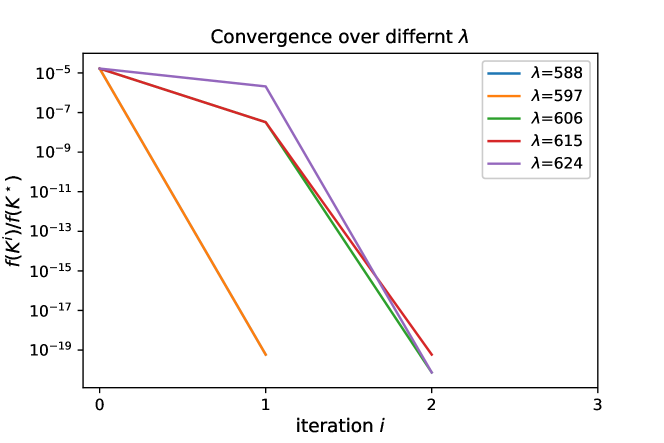
Sensitivity to initial and fixed stepsize choice. Note that we use the initial stepsize as a rule of thumb whereas the typical initial stepsize (Barzilai & Borwein, 1988; Wright et al., 2009; Park et al., 2020) does not depend on the regularization parameter . This stepsize choice is motivated by theoretical analysis (see Lemma 7 in Section 2.3) as well as empirical demonstration (see Fig. 1 in Section 4). This order of stepsize automatically scales well when experimenting over various s, alleviating iteration counts and leading to a faster algorithm in practice. It turns out that proximal gradient step is very sensitive to stepsizes, often leading to an unstable policy with or requiring a large number of iteration counts to converge. Therefore, we utilize linesearch over fixed stepsize choice.
Linesearch. We adopt a backtracking linesearch (See (Parikh et al., 2014)). Given , , , and the potential next iterate , it check if the following criterion (the stability and the decrease of the objective) is satisfied,
| (7) | ||||
where and is the spectral radius. Otherwise, it shrinks the stepsize by a factor of and check it iteratively until Eq. (7) is satisfied.
Stabilizing sequence of policy. We can start with a stable policy , meaning . For example, under the standard assumptions on , Riccati recursion provides a stable policy, the solution of standard LQR in Eq. (2). Then, satisfying the linesearch criterion in Eq. (7) subsequently, the rest of the policies are a stabilizing sequence.
Computational cost. The major cost incurs when solving the Lyapunov equations in the policy (and covariance) evaluation step. Note that if is stable, so does since they share the same eigenvalues. Under the stability, each Lyapunov equation in Eq. (4) has a unique solution with the computational cost (Jaimoukha & Kasenally, 1994; Li & White, 2002). Additionally, we can solve a sequence of Lyapunov equations with less cost, via using iterative methods with adopting the previous one (warm-start) or approximated one.
2.2.1 Regularizer and proximal operator
For various regularizers mentioned in Section 2.1, each has the closed-form solution for its proximal operator (Rockafellar, 1976; Parikh et al., 2014; Park et al., 2020). Here we only include a few representative examples and refer to the supplementary material for more examples.
Lemma 1 (Examples of proximal operator).
-
1.
Lasso. For ,
And we denote as a soft-thresholding operator.
-
2.
Nuclear norm. For ,
where is singular value decomposition with singular values .
-
3.
Proximity to . For ,
2.3 Convergence analysis of S-PI
Recall that , , is matrix norm, Frobenius norm, and smallest singular value, as mentioned in Section 1.1. First, we start with (local) smoothness and strong convexity around a stable policy. Here we regard a policy is stable if .
Assumptions. , , , and .
Lemma 2.
For stable , is smooth (in local) with
within local ball around where the radius is
And is strongly convex (in local) with
Then, we provide a proper stepsize that guarantees one iteration of proximal gradient step is still inside of the stable and (local) smooth ball .
Lemma 3.
Let . Then
holds for any where is given as
Next proposition describes that next iterate policy has the decrease in function value and is stable under sufficiently small stepsize.
Proposition 1.
Assume is stable. For any stepsize and next iterate ,
| (8) | |||
| (9) |
holds.
We also derive the bound on stepsize in Lemma 7, not dependent on iteration numbers.
Lemma 4.
Assume that is a stabilizing sequence and associated and are decreasing sequences. Then, Lemma 7 holds for
| (10) |
where
Now we prove that the S-PI in Algorithm 1 converges to the stationary point linearly.
Theorem 1.
from Algorithm 1 converges to the stationary point . Moreover, it converges linearly, i.e., after iterations,
Here, where
| (11) |
for some non-decreasing function on each argument.
Note that (the global bound on) stepsize is inversely proportional to , which motivates the initial stepsize in linesearch.
3 Toward a Model-Free Framework
In this section, we consider the scenario where the cost function and transition dynamic are unknown. Specifically in model-free setting, policy is directly learned from (trajectory) data without explicitly estimating the cost or transition model. In this section, we extend our Structured Policy Iteration (S-PI) to the model-free setting and prove its convergence.
3.1 Model-free Structured Policy Iteration (S-PI)
Note that, in model-free setting, model parameters and cannot be directly accessed, which hinders the direct computation of , , and accordingly. Instead, we adopt a smoothing procedure to estimate the gradient based on samples.
Model-free S-PI in Algorithm 3 consists of two steps: (1) policy evaluation step and (2) policy improvement step. In (perturbed) policy evaluation step, perturbation is uniformly drawn from the surface of the ball with radius , . These data are used to estimate the gradient via a smoothing procedure for the policy improvement step. With this approximate gradient, proximal gradient subroutine tries to decrease the objective while inducing the structure of policy. Comparing to (known-model) S-PI in Algorithm 1, one important difference is its usage of a fixed stepsize , rather than an adaptive stepsize from a backtracking linesearch that requires to access function value explicitly.
| (12) |
3.2 Convergence analysis of model-free S-PI
The outline of proof is as following: We first claim that for proper parameters (perturbation, horizon number, numbers of trajectory), the gradient estimate from the smoothing procedure is close enough to actual gradient with high probability. Next we demonstrate that approximate proximal gradient still converges linearly with high probability.
Theorem 2.
Suppose is finite, , and that has norm bounded by almost surly. Suppose the parameters in Algorithm 3 are chosen from
for some polynomials . Then, with the same stepsize in Eq. (20), there exist iteration at most such that with at least probability. Moreover, it converges linearly,
for the iteration , where .
Remark.
For (unregularized) LQR, the model-free policy gradient method (Fazel et al., 2018) is the first one that adopted a smoothing procedure to estimate the gradient. Similar to this, our model-free S-PI for regularized LQR also has several major challenges for deploying in practice. First one is that finding an initial policy with finite is non-trivial, especially when the open loop system is unstable, i.e., . Second one is its sensitivity to fixed stepsize as in the known model setting (in Section 2.2), wrong choice of which easily makes it divergent. Note that these two challenges hold over most of gradient based methods for LQR including policy gradient (Fazel et al., 2018), trust region policy optimization (TRPO) (Schulman et al., 2015), or proximal policy optimization (PPO) (Schulman et al., 2017). Last one is the joint sensitivity to multiple parameters , which may lead to high variance or large sub-optimality gap. On the other hand, REINFORCE (Williams, 1992) may suffer less variance, but with another potential difficulty: estimating the state-action value function . Moreover, it is not clear how to derive a structured policy. However, here we adopted smoothing procedures that enable us to theoretically analyze the convergence rate and parameter dependency.
4 Experiments
In experiments, we consider a LQR system for the purpose of validating the theoretical results and basic properties of the S-PI algorithm. As mentioned in Section 3.2, the simple example with an unstable open loop system, i.e., , is extremely sensitive to parameters even under known model setting, which may make it less in favor of the generic model-free RL approaches to deploy. Please note that our objective is total LQR cost-to-go in Eq. (2) more difficult than LQR cost-to-go averaged over time-horizon that some of works (Mania et al., 2018) considered. Under this difficulty, we demonstrate the properties of S-PI such as parameter sensitivity, convergence behaviors, and capability of balancing between LQR performance and policy structures. Finally, we illustrate the scalability of algorithms over various system dimensions.
4.1 Synthetic systems
In these experiments, we use the unstable Laplacian system (Recht, 2019).
Large Laplacian dynamics. where
and .
Synthetic system parameters. For the Laplacian system, we regard , , and dimension as small, medium, and large size of system. In addition, we experiment with Lasso regularizer over various .
4.2 Algorithm parameters
4.3 Results
We denote the stationary point from S-PI (at each ) as and the solution of the (unregularized) LQR as .
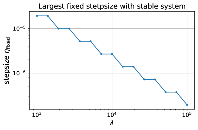
Dependency of stepsize on . Under the same problem but with different choices of weight , the largest fixed stepsize that demonstrates the sequence of stable systems, i.e., actually varies, as Lemma 7 implies. Fig. 1 shows that the largest stepsize diminishes as increases. This motivates the choice of the initial stepsize (in linesearch) to be inversely proportional to .
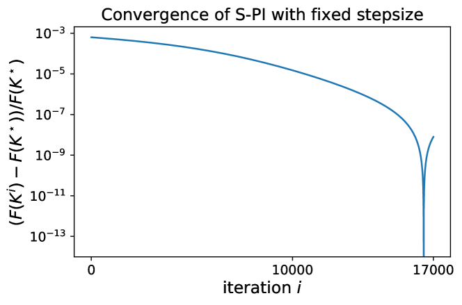
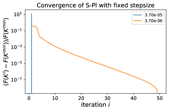
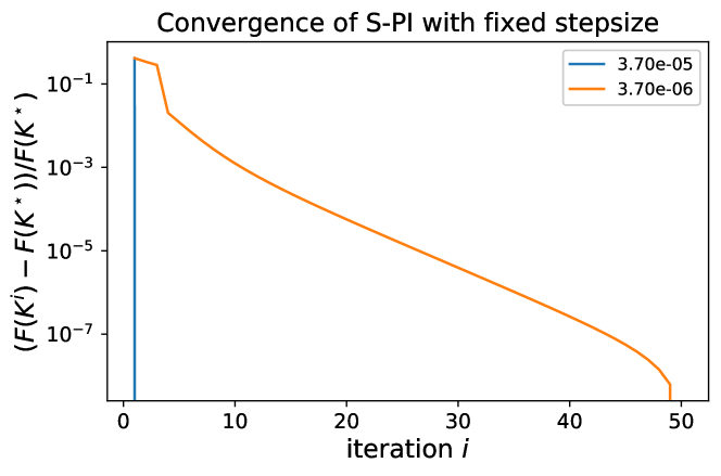
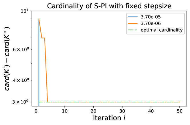
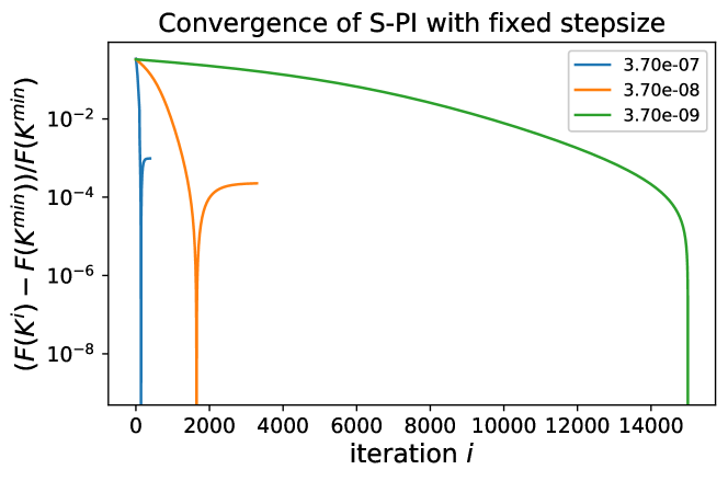
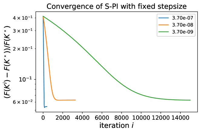
Convergence behavior and stepsize sensitivity. S-PI with a linesearh strategy converges very fast, within 2-3 iterations for most of the Laplacian system with dimension and weight . However, S-PI with fixed stepsize may perform with subtlety even though the fixed stepsize choice is common in typical optimization problems. In Fig. 2, S-PI with fixed stepsize for the small Laplacian system gets very close to optimal but begins to deviate after a certain amount of iterations. Note that it was performed over long iterations with small enough stepsize . Please refer to supplementary materials for more detailed results over various stepsizes. This illustrates that a linesearch strategy can be essential in S-PI (or even for the existing policy gradient method for LQR (Fazel et al., 2018)), even though the convergence analysis was shown with some fixed stepsize (but difficult to compute in practice).
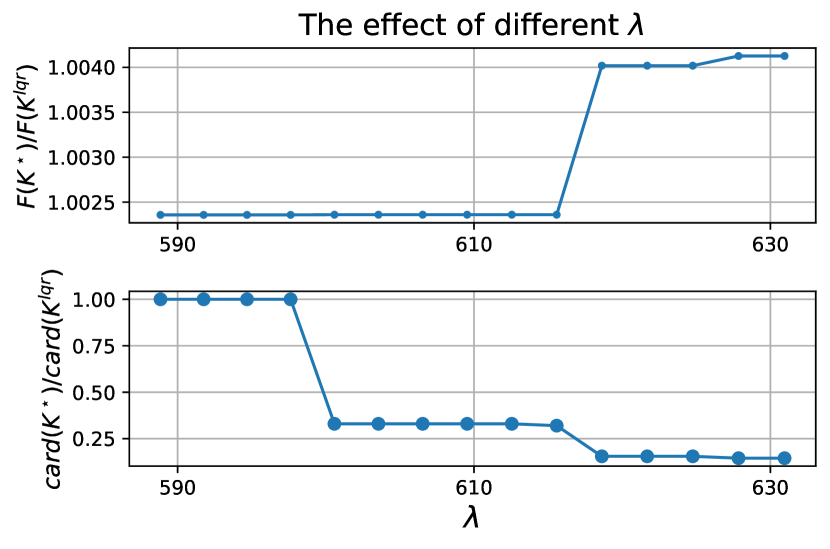
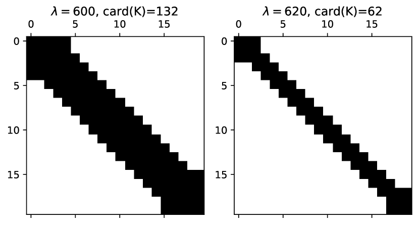
Trade off between LQR performance and structure . In Fig. 3 for a medium size Laplacian system, we show that as increases, the LQR cost increases whereas cardinality decreases (sparsitiy is improved). Note that the LQR performance barely changes (or is slightly worse) for but the sparsity is significantly improved by more than . In Fig. 4, we show the sparsity pattern (location of non-zero elements) of the policy matrix with and .
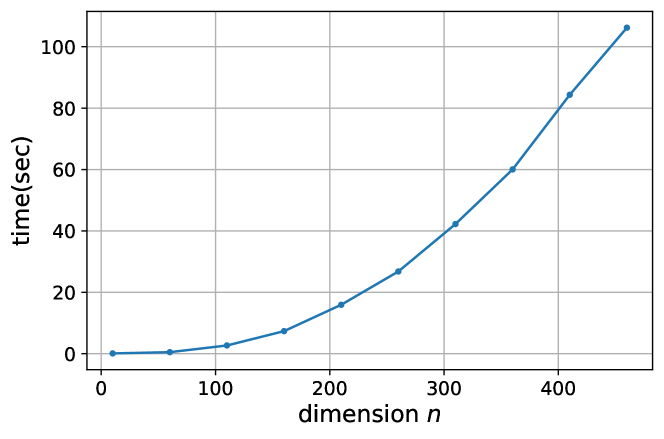
Scalability & runtime performance. In Fig. 5, we report the runtime for Laplacian system of . Notably, it shows the scalability of S-PI, as it takes less than 2 minutes to solve a large system with dimensions, where we used a MacBook Air (with a 1.3 GHz Intel Core i5 CPU) for experiments. These results demonstrate its applicability to large-scale problems in practice.
5 Conclusion and Discussion
In this paper, we formulated a regularized LQR problem to derive a structured linear policy and provided an efficient algorithm, Structured Policy Iteration (S-PI). We proved that S-PI guarantees to converge linearly under a proper choice of stepsize, keeping the iterate within the set of stable policy as well as decreasing the objective at each iteration. In addition, we extended S-PI for model-free setting, utilizing a smoothing procedure. We also proved its convergence guarantees with high probability under a proper choice of parameters including stepsize, horizon counts, trajectory counts, etc. In the experiments, we examined some basic properties of the S-PI such as sensitivity on stepsize and regularization parameters to convergence behaviors, which turned out to be more critical than typical optimization problems. Lastly, we demonstrated that our method is effective in terms of balancing the quality of solution and structures.
We leave for future work the practical application of other penalty functions such as low-rank and proximity regularization. There are also new extensions on using proximal Newton or proximal natural gradient method as a subroutine, beyond what was developed in S-PI in Section 2, which could be further analyzed. Even though model-free algorithm for regularized LQR was suggested with theoretical guarantees, it is extremely difficult to deploy in practice, like most of model-free approaches for LQR. Finally, developing algorithm reducing variance for (regularized) LQR, possibly like (Papini et al., 2018; Park & Ryu, 2020), as well as some practical rule of thumb on the choice of hyper-parameters is another class of important problems to tackle toward model-free settings.
We described a new class of discrete time LQR problems that have yet to be studied theoretically and practically. And we discussed and demonstrated how such problems can be of practical importance despite them not being well-studied in the literature.While a few application were covered for this new class of problems, each of these contributions would open up our framework to new potential applications, providing additional benefits to future research on this topic.
References
- Abbasi-Yadkori & Szepesvári (2011) Abbasi-Yadkori, Y. and Szepesvári, C. Regret bounds for the adaptive control of linear quadratic systems. In Proceedings of the 24th Annual Conference on Learning Theory, pp. 1–26, 2011.
- Al Borno et al. (2012) Al Borno, M., De Lasa, M., and Hertzmann, A. Trajectory optimization for full-body movements with complex contacts. IEEE transactions on visualization and computer graphics, 19(8):1405–1414, 2012.
- Anderson & Moore (2007) Anderson, B. D. and Moore, J. B. Optimal control: linear quadratic methods. Courier Corporation, 2007.
- Balakrishnan & Vandenberghe (2003) Balakrishnan, V. and Vandenberghe, L. Semidefinite programming duality and linear time-invariant systems. IEEE Transactions on Automatic Control, 48(1):30–41, 2003.
- Barzilai & Borwein (1988) Barzilai, J. and Borwein, J. M. Two-point step size gradient methods. IMA journal of numerical analysis, 8(1):141–148, 1988.
- Bellman et al. (1954) Bellman, R. et al. The theory of dynamic programming. Bulletin of the American Mathematical Society, 60(6):503–515, 1954.
- Bertsekas & Shreve (2004) Bertsekas, D. P. and Shreve, S. Stochastic optimal control: the discrete-time case. 2004.
- Bertsekas & Tsitsiklis (1996) Bertsekas, D. P. and Tsitsiklis, J. N. Neuro-dynamic programming, volume 5. Athena Scientific Belmont, MA, 1996.
- Bertsekas et al. (1995) Bertsekas, D. P., Bertsekas, D. P., Bertsekas, D. P., and Bertsekas, D. P. Dynamic programming and optimal control, volume 1. Athena scientific Belmont, MA, 1995.
- Bradtke et al. (1994) Bradtke, S. J., Ydstie, B. E., and Barto, A. G. Adaptive linear quadratic control using policy iteration. In Proceedings of 1994 American Control Conference-ACC’94, volume 3, pp. 3475–3479. IEEE, 1994.
- Conn et al. (2009) Conn, A. R., Scheinberg, K., and Vicente, L. N. Introduction to derivative-free optimization, volume 8. Siam, 2009.
- Costa et al. (2006) Costa, O. L. V., Fragoso, M. D., and Marques, R. P. Discrete-time Markov jump linear systems. Springer Science & Business Media, 2006.
- De Farias & Van Roy (2003) De Farias, D. P. and Van Roy, B. The linear programming approach to approximate dynamic programming. Operations research, 51(6):850–865, 2003.
- Dean et al. (2017) Dean, S., Mania, H., Matni, N., Recht, B., and Tu, S. On the sample complexity of the linear quadratic regulator. Foundations of Computational Mathematics, pp. 1–47, 2017.
- Elmaghraby (1993) Elmaghraby, S. E. Resource allocation via dynamic programming in activity networks. European Journal of Operational Research, 64(2):199–215, 1993.
- Fazel et al. (2018) Fazel, M., Ge, R., Kakade, S. M., and Mesbahi, M. Global convergence of policy gradient methods for the linear quadratic regulator. arXiv preprint arXiv:1801.05039, 2018.
- Flaxman et al. (2004) Flaxman, A. D., Kalai, A. T., and McMahan, H. B. Online convex optimization in the bandit setting: gradient descent without a gradient. arXiv preprint cs/0408007, 2004.
- Florentin (1961) Florentin, J. J. Optimal control of continuous time, markov, stochastic systems. International Journal of Electronics, 10(6):473–488, 1961.
- Hewer (1971) Hewer, G. An iterative technique for the computation of the steady state gains for the discrete optimal regulator. IEEE Transactions on Automatic Control, 16(4):382–384, 1971.
- Ibrahimi et al. (2012) Ibrahimi, M., Javanmard, A., and Roy, B. V. Efficient reinforcement learning for high dimensional linear quadratic systems. In Advances in Neural Information Processing Systems, pp. 2636–2644, 2012.
- Jaimoukha & Kasenally (1994) Jaimoukha, I. M. and Kasenally, E. M. Krylov subspace methods for solving large lyapunov equations. SIAM Journal on Numerical Analysis, 31(1):227–251, 1994.
- Kakade (2002) Kakade, S. M. A natural policy gradient. In Advances in neural information processing systems, pp. 1531–1538, 2002.
- Kalman (1964) Kalman, R. E. When is a linear control system optimal? Journal of Basic Engineering, 86(1):51–60, 1964.
- Kumar et al. (2016) Kumar, V., Todorov, E., and Levine, S. Optimal control with learned local models: Application to dexterous manipulation. In 2016 IEEE International Conference on Robotics and Automation (ICRA), pp. 378–383. IEEE, 2016.
- Lancaster & Rodman (1995) Lancaster, P. and Rodman, L. Algebraic riccati equations. Clarendon press, 1995.
- Lau et al. (1972) Lau, R., Persiano, R., and Varaiya, P. Decentralized information and control: A network flow example. IEEE Transactions on Automatic Control, 17(4):466–473, 1972.
- Laub (1979) Laub, A. A schur method for solving algebraic riccati equations. IEEE Transactions on automatic control, 24(6):913–921, 1979.
- Lazic et al. (2018) Lazic, N., Boutilier, C., Lu, T., Wong, E., Roy, B., Ryu, M. K., and Imwalle, G. Data center cooling using model-predictive control. In Advances in Neural Information Processing Systems (NeurIPS), pp. 3818–3827, 2018.
- Lewis et al. (2012) Lewis, F. L., Vrabie, D., and Syrmos, V. L. Optimal control. 3rd ed. Hoboken, NJ: John Wiley Sons. , 2012.
- Li & White (2002) Li, J.-R. and White, J. Low rank solution of lyapunov equations. SIAM Journal on Matrix Analysis and Applications, 24(1):260–280, 2002.
- Lin et al. (2012) Lin, F., Fardad, M., and Jovanović, M. R. Sparse feedback synthesis via the alternating direction method of multipliers. In 2012 American Control Conference (ACC), pp. 4765–4770. IEEE, 2012.
- Mania et al. (2018) Mania, H., Guy, A., and Recht, B. Simple random search provides a competitive approach to reinforcement learning. arXiv preprint arXiv:1803.07055, 2018.
- Mania et al. (2019) Mania, H., Tu, S., and Recht, B. Certainty equivalent control of lqr is efficient. arXiv preprint arXiv:1902.07826, 2019.
- Mnih et al. (2015) Mnih, V., Kavukcuoglu, K., Silver, D., Rusu, A. A., Veness, J., Bellemare, M. G., Graves, A., Riedmiller, M. A., Fidjeland, A., Ostrovski, G., Petersen, S., Beattie, C., Sadik, A., Antonoglou, I., King, H., Kumaran, D., Wierstra, D., Legg, S., and Hassabis, D. Human-level control through deep reinforcement learning. Nature, 518(7540):529–533, 2015.
- Nerlove & Arrow (1962) Nerlove, M. and Arrow, K. J. Optimal advertising policy under dynamic conditions. Economica, pp. 129–142, 1962.
- Nesterov & Spokoiny (2017) Nesterov, Y. and Spokoiny, V. Random gradient-free minimization of convex functions. Foundations of Computational Mathematics, 17(2):527–566, 2017.
- O’Donoghue et al. (2011) O’Donoghue, B., Wang, Y., and Boyd, S. Min-max approximate dynamic programming. In 2011 IEEE International Symposium on Computer-Aided Control System Design (CACSD), pp. 424–431. IEEE, 2011.
- Papini et al. (2018) Papini, M., Binaghi, D., Canonaco, G., Pirotta, M., and Restelli, M. Stochastic variance-reduced policy gradient. arXiv preprint arXiv:1806.05618, 2018.
- Parikh et al. (2014) Parikh, N., Boyd, S., et al. Proximal algorithms. Foundations and Trends® in Optimization, 1(3):127–239, 2014.
- Park & Ryu (2020) Park, Y. and Ryu, E. K. Linear convergence of cyclic saga. Optimization Letters, pp. 1–16, 2020.
- Park et al. (2019) Park, Y., Mahadik, K., Rossi, R. A., Wu, G., and Zhao, H. Linear quadratic regulator for resource-efficient cloud services. In Proceedings of the ACM Symposium on Cloud Computing, pp. 488–489, 2019.
- Park et al. (2020) Park, Y., Dhar, S., Boyd, S., and Shah, M. Variable metric proximal gradient method with diagonal barzilai-borwein stepsize. In ICASSP 2020-2020 IEEE International Conference on Acoustics, Speech and Signal Processing (ICASSP), pp. 3597–3601. IEEE, 2020.
- Powell (2007) Powell, W. B. Approximate Dynamic Programming: Solving the curses of dimensionality, volume 703. John Wiley & Sons, 2007.
- Recht (2019) Recht, B. A tour of reinforcement learning: The view from continuous control. Annual Review of Control, Robotics, and Autonomous Systems, 2:253–279, 2019.
- Rockafellar (1976) Rockafellar, R. T. Monotone operators and the proximal point algorithm. SIAM journal on control and optimization, 14(5):877–898, 1976.
- Sandell et al. (1978) Sandell, N., Varaiya, P., Athans, M., and Safonov, M. Survey of decentralized control methods for large scale systems. IEEE Transactions on automatic Control, 23(2):108–128, 1978.
- Sarimveis et al. (2008) Sarimveis, H., Patrinos, P., Tarantilis, C. D., and Kiranoudis, C. T. Dynamic modeling and control of supply chain systems: A review. Computers & Operations Research, 35(11):3530–3561, 2008.
- Schulman et al. (2015) Schulman, J., Levine, S., Abbeel, P., Jordan, M., and Moritz, P. Trust region policy optimization. In International conference on machine learning, pp. 1889–1897, 2015.
- Schulman et al. (2017) Schulman, J., Wolski, F., Dhariwal, P., Radford, A., and Klimov, O. Proximal policy optimization algorithms. arXiv preprint arXiv:1707.06347, 2017.
- Silver et al. (2016) Silver, D., Huang, A., Maddison, C. J., Guez, A., Sifre, L., van den Driessche, G., Schrittwieser, J., Antonoglou, I., Panneershelvam, V., Lanctot, M., Dieleman, S., Grewe, D., Nham, J., Kalchbrenner, N., Sutskever, I., Lillicrap, T. P., Leach, M., Kavukcuoglu, K., Graepel, T., and Hassabis, D. Mastering the game of go with deep neural networks and tree search. Nature, 529(7587):484–489, 2016.
- Sutton et al. (1998) Sutton, R. S., Barto, A. G., et al. Introduction to reinforcement learning, volume 2. MIT press Cambridge, 1998.
- Tassa et al. (2012) Tassa, Y., Erez, T., and Todorov, E. Synthesis and stabilization of complex behaviors through online trajectory optimization. In 2012 IEEE/RSJ International Conference on Intelligent Robots and Systems, pp. 4906–4913. IEEE, 2012.
- Tu & Recht (2017) Tu, S. and Recht, B. Least-squares temporal difference learning for the linear quadratic regulator. arXiv preprint arXiv:1712.08642, 2017.
- Wang & Davison (1973) Wang, S.-H. and Davison, E. On the stabilization of decentralized control systems. IEEE Transactions on Automatic Control, 18(5):473–478, 1973.
- Watkins & Dayan (1992) Watkins, C. J. and Dayan, P. Q-learning. Machine learning, 8(3-4):279–292, 1992.
- Williams (1992) Williams, R. J. Simple statistical gradient-following algorithms for connectionist reinforcement learning. Machine learning, 8(3-4):229–256, 1992.
- Wonham (1970) Wonham, W. M. Random differential equations in control theory. 1970.
- Wright et al. (2009) Wright, S. J., Nowak, R. D., and Figueiredo, M. A. Sparse reconstruction by separable approximation. IEEE Transactions on Signal Processing, 57(7):2479–2493, 2009.
- Wytock & Kolter (2013) Wytock, M. and Kolter, J. Z. A fast algorithm for sparse controller design. arXiv preprint arXiv:1312.4892, 2013.
Appendix A Discussion on Non-convexity of Regularized LQR.
From Lemma 2 and appendix in (Fazel et al., 2018), unregularized objective is known to be not convex, quasi-convex, nor star-convex, but to be gradient dominant, which gives the claim that all the stationary points are optimal as long as . However, in regularized LQR, this claim may not hold.
To see this claim that all stationary points may not be global optimal, let’s define regularized LQR with where is the solution of the Riccati algorithm. We know that is the global optimal. Assume there is another distinct stationary point (like unregularized LQR) . Then, is always less than . If not,i.e., , then holds and this is contradiction, showing all stationary points is not global optimal like unregularized LQR. Whether regularized LQR has only one stationary point or not is still an open question.
Appendix B Additional Examples of Proximal Operators
Assume are positive numbers. We denote as its th element or as its th block under an explicit block structure, and .
-
•
Group lasso. For a group lasso penalty with ,
-
•
Elastic net For a elastic net ,
-
•
Nonnegative constraint. Let be the nonnegative constraint. Then
-
•
Simplex constraint Let be the simplex constraint. Then for ,
Here, is the solution satisfying , which can be found efficiently via bisection.
Appendix C Proof for Convergence Analysis of S-PI
Let’s define . We often adopt and modify several techincal Lemmas like perturbation analysis from (Fazel et al., 2018).
Lemma 5 (modification of Lemma 16 in (Fazel et al., 2018)).
Suppose is stable and is in the ball , i.e.,
where the radius is
Then
| (13) |
Lemma 6 (Lemma 2 restated).
For with stable , is locally smooth with
within local ball around
And is (globally) strongly convex with
In addition, is stable for all .
Proof.
First, we describe the terms with Talyor expansion
The second order term is (locally) upper bounded by
where (a) holds due to Lemma 5
within a ball .
On the other hand,
where (b) hold due to and .
Therefore, the second order term is (locally) bounded by
where
∎
Lemma 7 (Lemma 3 restated).
Let . Then
holds for any where is given as
Proof.
For lasso, let be a soft-thresholding operator.
where the last inequality holds iff
For nuclear norm,
Therefore,
where the last inequality holds iff
For the third regulazer,
where (a) holds from the closed solution of proximal operator in Lemma 1(in main paper) and (b) holds due to and . Therefore, using this inequality gives
where the last inequality holds iff
∎
Lemma 8.
For any , let where . Then, for any ,
| (14) |
holds.
Proof.
For with any and any , we have
where (a) holds due to convexity of , (b) holds due to the property of subgradient on proximal operator. Next, for any , holds from Lemma 7 and thus is locally smooth. Therefore
| (15) |
where (c) holds due to -smoothness for , (d) holds by , (e) holds due to -strongly convexity at . And note that Substituting in (15) is equivalent to linesearch criterion in Eq. (8) (in main paper), which will be satisfied for small enough stepsize after linesearch iterations.
Adding two inequalities above gives
| (16) | ||||
∎
Proposition 2 (Proposition 1 restated).
Assume is stable. For any stepsize and next iterate ,
| (17) | |||
| (18) |
holds.
Proof.
Lemma 9 (Lemma 4 restated).
Assume that is a stabilizing sequence and associated and are decreasing sequences. Then, Lemma 7 holds for
| (19) |
where
Proof.
For the proof, we derive the global bound on and , then plug these into Lemma 7 to complete our claim. First, we utilize the derivation of the upperbound on and in (Fazel et al., 2018) under the assumption of decreasing sequence as follows,
From this, we have
holds where we used the fact that and . Now we complete the proof by also providing .Since is bounded as
where the last inequality holds due to .
∎
Proposition 3.
Let be the stepsize from backtracking linesearch at -th iteration. After iterations, it converges to a stationary point satisfying
where , iff . Moreover,
where is a function non-decreasing on each argument.
Proof.
From Lemma 2,
Reordering terms and averaging over iterations give
And LHS is lower bounded by
giving the desirable result. Moreover, it converges to the stationary point since .
Now the remaining part is to bound the stepsize. Note that the stepsize after linesearch satisfies
First we bound as follows,
Next, about the bound on , we already have from Lemma 9.
Note that both of bounds are proportional to and , and inverse-proportional to and .
Therefore
for some that is non-decreasing on each argument.
∎
Theorem 3 (Theorem 1 restated).
from Algorithm 1 converges to the stationary point . Moreover, it converges linearly, i.e., after iterations,
Here, where
| (20) |
for some non-decreasing function on each argument.
Proof.
Corollary 2.
Proof.
This is immediate from Theorem 3, using the inequality and by taking the logarithm. ∎
Appendix D Proof for Convergence Analysis of Model-free S-PI
Lemma 10 (Lemma 30 in (Fazel et al., 2018)).
There exists polynomials , , , such that, when , and , the gradient estimate given in Eq. (13) of Algorithm 3 satisfies
with high probability (at least .
Theorem 4 (Theorem 2 restated).
Suppose is finite, , and that has norm bounded by almost surly. Suppose the parameters in Algorithm 3 are chosen from
for some polynomials . Then, with the same stepsize in Eq. (20), Algorithm 3 converges to its stationary point with high probability. In particular, there exist iteration at most such that with at least probability. Moreover, it converges linearly,
for the iteration , where .
Proof.
Let be the error bound we want to obtain, i.e., where is the policy from Algorithm 3 after iterations.
For a notational simplicity, we denote and see the contraction of the proximal operator at th iteration. First we use Lemma 10 to claim that, with high probability, for long enough numbers of trajactory and horizon where is specified later.
Second, we bound the error after one iteration of approximated proximal gradient step at the policy , i.e., . Here let be the next iterate using approximate gradient and be the one using the exact gradient .
where we use the fact that proximal operator is non-expansive and holds for proper parameter choices (the claim in the previous paragraph).
Third, we find the contractive upperbound after one iteration using approximated proximal gradient.
Let’s assume under current policy. Then, taking square on both sides gives
where we used , , and the assumption. Choosing results in
with high probability . This says the approximate proximal gradient is contractive, decreasing in error after one iteration. Keep applying this inequality, we get
as long as .
This says that there must exist the iteration s.t.
| (21) |
Now we claim this is at most . To prove this claim, suppose it is not, i.e., . Then, for ,
which is a contradiction to (21).
Finally, we show the probability that this event occurs. Note that all randomness occur when estimating gradient within error. From union bound, it occurs at least . And this is bounded below by
∎
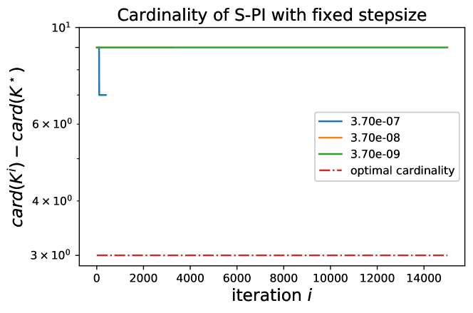
Appendix E Additional Experiments on Stepsize Sensitivity
In this section, we scrutinize the convergence behaviors of S-PI under some fixed stepsize. For a very small Laplacian system with Lasso penalty , we run S-PI over a wide range of stepsizes. For stepsize larger than , S-PI diverges and thus is ran under stepsizes smaller than . Let be the policy where the objective value attains its minimum among overall iterates and be the policy from S-PI with linesearch (non-fixed stepsize). Here the cardinality of the optimal policy is . For a fixed stepsizes in , S-PI converges to the optimal. In Figure 7, the objective value monotonically decreases and the policy converges to optimal one based on errors and cardinality. However, for smaller stepsize like , Figure 8 shows that S-PI still converges but does not show monotonic behaviors nor converges to the optimal policy. These figures demonstrate the sensitivity of a stepsize when S-PI is used under a fixed stepsize, rather than linesearch. Like in Figure 8, the algorithm can be unstable under fixed stepsize because the next iterate may not satisfy the stability condition and or are not guaranteed for a monotonic decrease. Moreover, this instability may lead to another stationary point even when the iterate falls in some stable policy region after certain iterations. This not only demonstrates the importance of lineasearch due to its sensitivity on the stepsize, but may provide the evidence for why other policy gradient type of methods for LQR did not perform well in practice.