Study of Phase Reconstruction Techniques applied to Smith-Purcell Radiation Measurements
Abstract
Measurements of coherent radiation at accelerators typically give the absolute value of the beam profile Fourier transform but not its phase. Phase reconstruction techniques such as Hilbert transform or Kramers Kronig reconstruction are used to recover such phase. We report a study of the performances of these methods and how to optimize the reconstructed profiles.
1 Longitudinal bunch profile measurement at particle accelerators
On a particle accelerator the longitudinal profiles of a particle bunch can not easily be measured. Several indirect measurement techniques have been established relying on the measurement of the spectrum of radiation emitted by the bunch either when it crosses a different material [1] or when it passes near a different material [2, 3]. This emitted spectrum encode the longitudinal profile through the relation:
| (1) |
where is the emitted intensity as a function of the wavelength . is the intensity of the signal emitted by a single particle and is a form factor that encodes the longitudinal and transverse shape of the particle bunch. Recovering the longitudinal profile requires to invert this equation however this is not straightforward as the information about the phase of the form factor can not be measured and therefore is not available.
A phase reconstruction algorithm must therefore be used to recover this phase. Several methods exist (see for example [4]). In this article we describe how we implemented two of these methods and compared their performances.
2 Reconstruction methods
When it is only possible to measure the amplitude of the complex signal, it is necessary to recover the phase of the available data. We assume that the function of the longitudinal beam density is analytical. For an analytic function this is easier because the real and imaginary part are not completely independent. The Kramers-Kronig relations [4] helps restore the imaginary part of an analytic function from its real part and vice versa.
To recover the phase from the amplitude, the function should be written as: with its amplitude and its phase. The Kramers-Kronig relations can then be applied as follows:
| (2) |
The basis of this relationship are the Cauchy-Riemann conditions (analyticity of function).
In some cases this phase can also be obtained simply by using the Hilbert transform of the spectrum:
| (3) |
As the Hilbert transform (H) is related to the Fourier transform ():
| (4) |
the calculation of phase can use an optimised FFT code and is therefore much faster than calculating the Kramers-Kronig’s integral. We implemented in Matlab these two different phase reconstruction methods. The Hilbert transform method has the advantage of being directly implemented in Matlab, allowing a much faster computing.
3 Description of the simulations
To test the performance of these methods we created a small Monte-Carlo program that randomly simulates profiles () made of the combination of 5 gaussians according to the formula where and , and are random numbers with , , and . The values of these ranges have been chosen to generate profiles that are not disconnected (that is profiles whose intensity drops to almost zero between two peaks) without being perfect gaussian. We checked that our conclusions are valid across this range.
Using this formula we generated 1000 profiles, then took the absolute value of their Fourier transform and sampled at a limited number of frequency points () as would be done with a real experiment in which the number of measurement points is limited (limited number of detectors or limited number of scanning steps).
To estimate the performance of the reconstruction several estimators are available. We choose to use the , defined as follow:
| (5) |
where is the observed value , is the expected (simulated) value, is the weight of the point, N is the number of points.
However two very similar profiles but with a slight offset, will give a worse than a profile with oscillations (see figure 1). This can be partly mitigated (in the case of horizontal offset) by offsetting one profile with respect to the other until the is minimized.
Also we decided to look at the FWHM which was generalized as FWXM where is the fraction of the maximum value at which the full width of the reconstructed profile was calculated (with this definition the standard FWHM is noted FW0.5M). We created an estimator defined as follow:
| (6) |
where and are the FWXM of the original and reconstructed profiles respectively.
Here two profiles that are similar but slightly offset (in position or amplitude) will nevertheless return good values of this estimator despite returning a rather large .
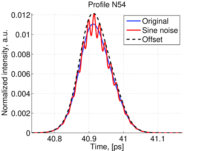
; For profile with sine noise: FW0.1M=0.0241, FW0.2M=0.044 FWHM=0.0621 FW0.8M=0.1849 FW0.9M=0.3619. As FWXM calculated from top of profile, for all profiles FWXM=0.
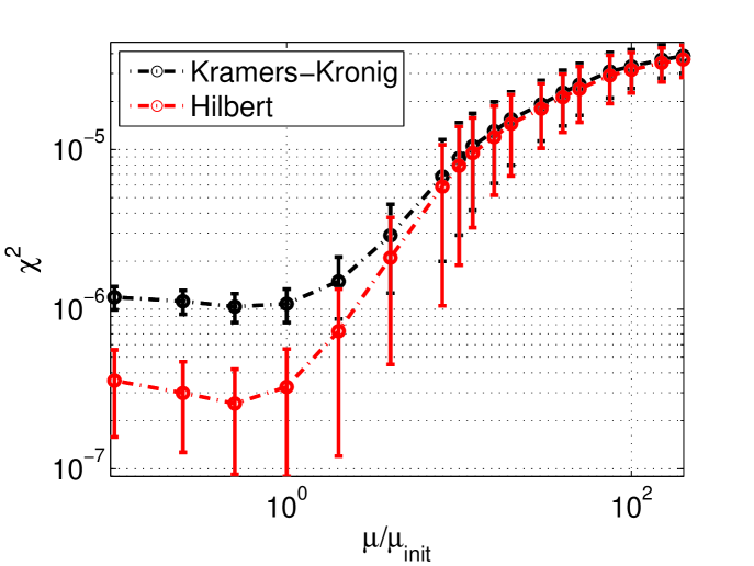
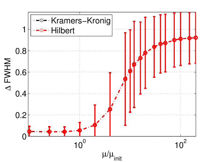
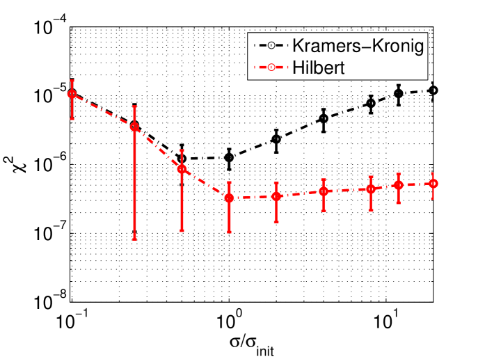
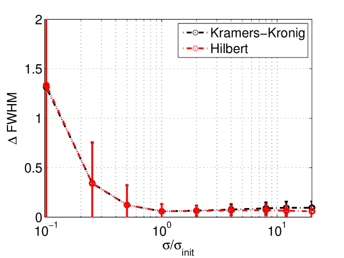
To ensure that the choice of the parameters and for the simulations does not bias significantly the results, their value has been varied and this is shown in figure 2.
Different distributions have been used for the frequencies : linear, logarithmic, triple-sine. In most sampling schemes we used 33 frequencies to make it comparable with the Triple-sine distribution used in [5]. These sampling schemes are defined as follow:
-
•
Triple-sine This sampling matches that of the E-203 experiment at FACET [5]. Eleven detectors are located every around the interaction point and 3 different sets of wavelengths are used, giving the following distribution:
(7) with and varying between and by steps of .
-
•
Linear sampling Here sampling points are distributed uniformly. The first and last points of sampling are the first () and last () points used in the Triple-sine sampling. The following formula gives the sampling frequencies:
(8) -
•
Logarithmic sampling. Here sampling points are distributed logarithmically:
(9) For this sampling also the first and last points are the same as in Triple-sine sampling.
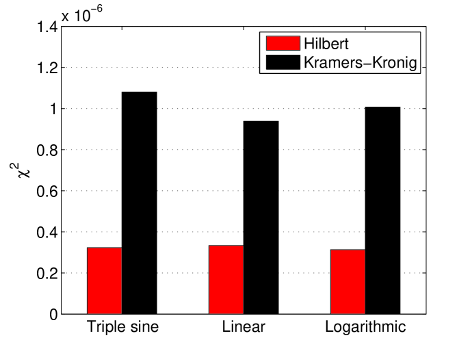
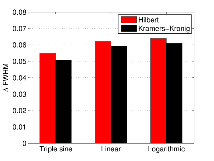
The study of the sampling is important, as it shows the best position of the detectors and also how to optimize the system. Linearly sampled spectrum gives the best result as shown in figure 3.
However, the linear sampling may not be practical to realize in a the real world. One needs to take into account the spatial size of the detectors (about 10 degrees in the case of E-203) and there is also a limit on the start and end points of detectors location (35-145 degrees for E-203). So linear sampling at a wide range of frequencies is impossible with this number of points. An investigation of how many linear sampling points can be used for a given angle difference between detectors shows that such physical constraints reduce strongly the number of detectors that can be used. Figure 4 shows examples of detector positions. The position of the red points is calculated using formula 7 and blue are possible detector positions which don’t break the minimum detector distance (MDD) given on top of each plot.
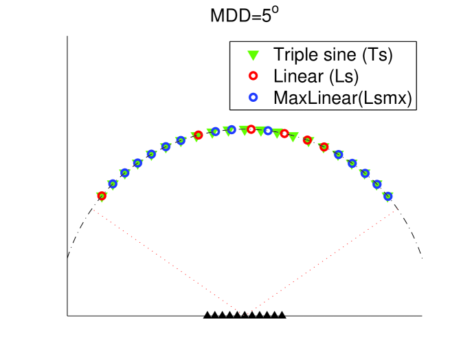
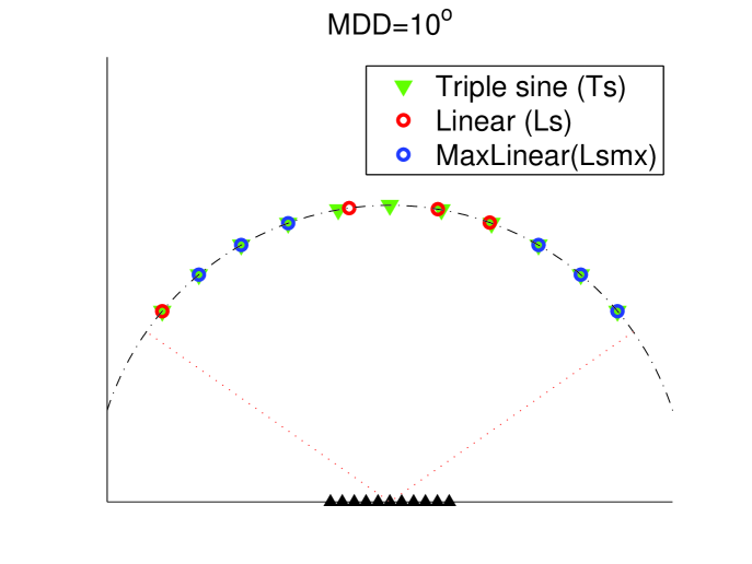
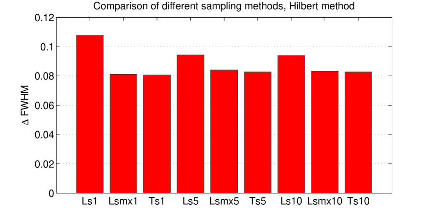
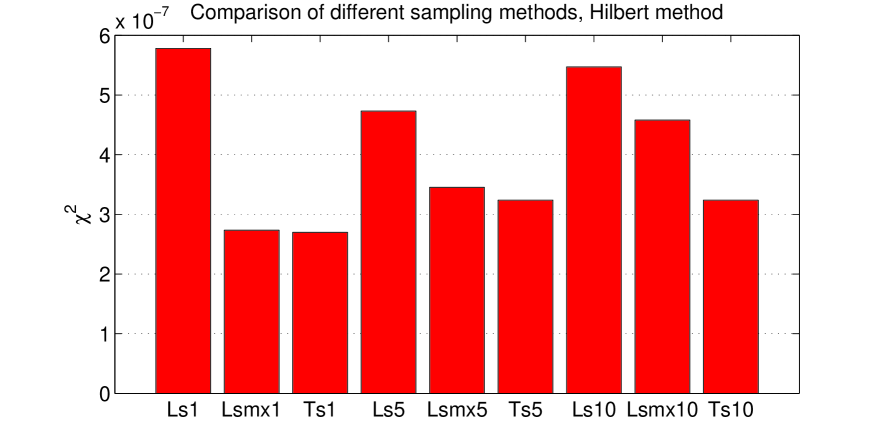
Figure 5 shows a comparison of the performances achieved with such positioning for different MDD. In each case the triple sine sampling (Ts) is better than the linear sampling (Ls) and close from the maximum number of detectors with linear sampling (Lsmx). So the Ts configuration is favored and will be used in the rest of this paper. The comparison between Ts1, Ts5 and Ts10 shows that reconstruction performances are limited by the MDD.
The choice of 33 frequencies for the sampling of the spectrum was made to match the current layout used on E-203. However it is important to check if there is an optimum value. To perform this check we used the same simulations and the same simulated spectrum but sampled with 3 to 140 points. The effect of changing the sampling frequencies on the is shown in figure 6. This study uses Triple sine sampling with 1000 profiles for each point and both reconstruction method.
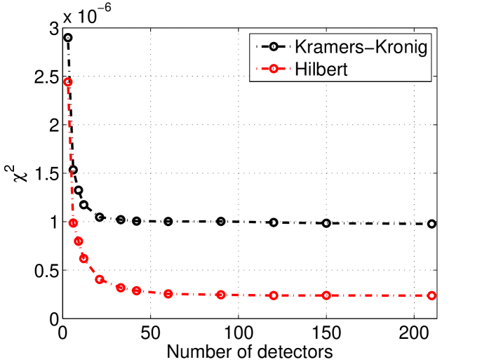
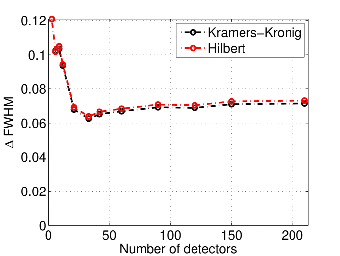
It can be seen at figure 6 that beyond about 33 sampling points the gain on the reconstructed is marginal.
After applying the sampling procedure the data need to be interpolated and extrapolated to have a larger number of points in the spectrum. Interpolation is done using Piecewise Cubic Hermite Interpolating Polynomial (PCHIP) [8], as suggested in [7]. The interpolation function must satisfy the following criteria: it must conserve the slope at the two endpoints (to have a continuous derivative) and respects monotonicity. PCHIP interpolation has been chosen as it matches these requirements.
For low frequency extrapolation two methods have been investigated: Gaussian or Taylorian.
In the Gaussian method, we defined the extrapolation as follow:
| (10) |
Where is the extrapolated spectrum at low frequency and the constants A, B, and C were chosen from the following conditions:
-
•
-
•
-
•
The extrapolation relies in the fact that according to the central limit theorem in the time space the expected profile is Gaussian-like and in the frequency space it will also be Gaussian.
The other extrapolation method is based on Taylor expansion with the following definition:
| (11) |
Approximation to the 4th order gives the following low frequency (LF) extrapolation:
| (12) |
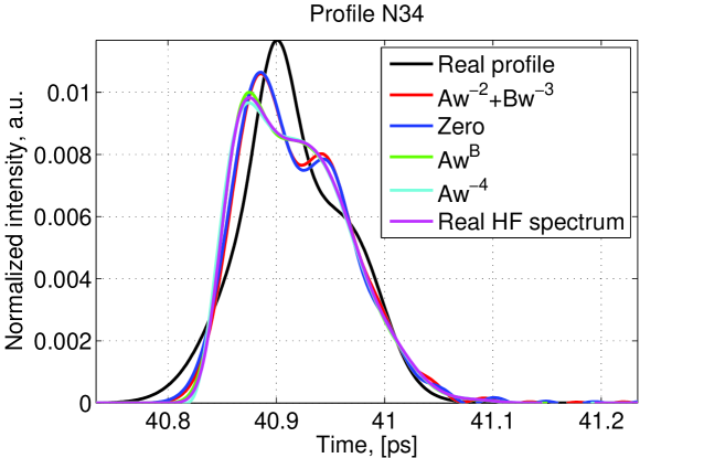
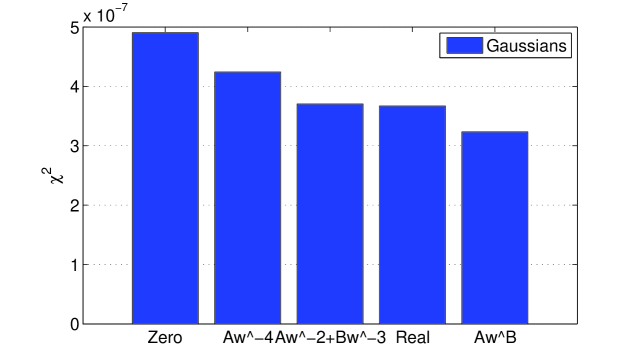
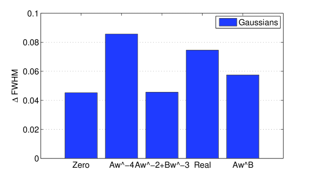
Conditions for the constants A, B and C are the same. Comparison of different LF extrapolation can be found in figure 7 and the performances of these methods in figure 8.
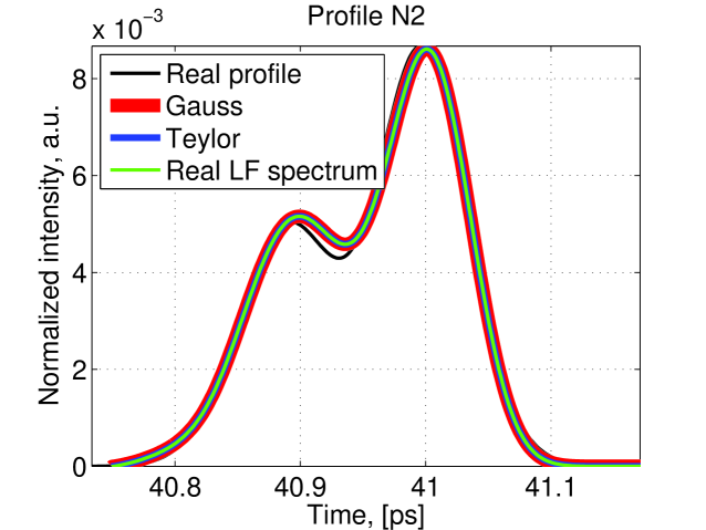
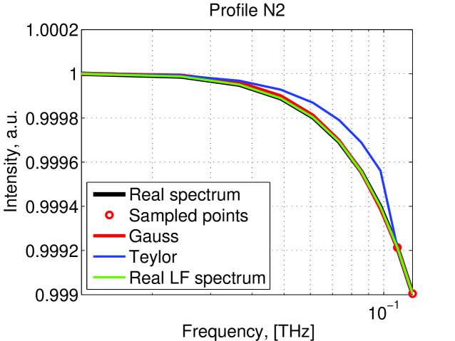
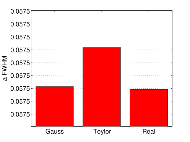
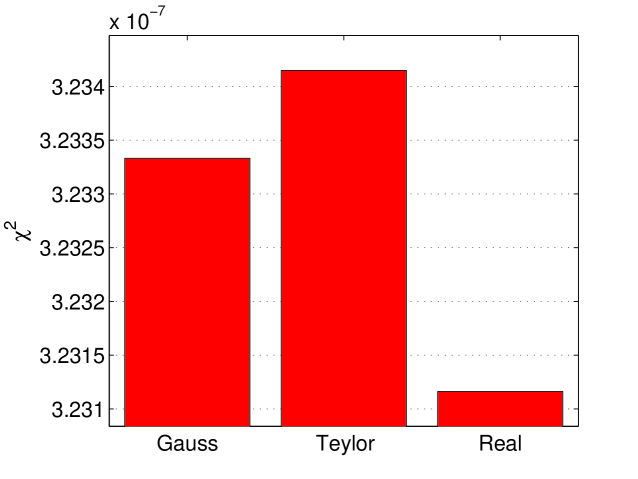
In the rest of this paper we used the Gaussian method.
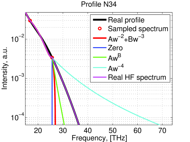
Several high frequency (HF) extrapolation methods were also tested. The most common [7, 10] is :
| (13) |
where is the extrapolated spectrum at high frequency and , where is spectrum value of final point .
The second method uses the same consideration as in Lai and Sievers [9]: Assuming that the bunch size is finite with two end points at and at then the longitudinal charge distribution () must follow . An integration by parts gives :
| (14) |
The first term vanishes because of the boundary conditions, so for large , is proportional to and two conditions have to be matched :
-
•
-
•
where is the last sampled point of the spectrum. To satisfy the boundary condition two constants are needed, giving a two-terms extrapolation :
| (15) |
or extrapolation with degree of frequency as free parameter:
| (16) |
where the A and B – coefficients which are calculated from the last data samples and the boundary conditions as follow:
-
•
-
•
The requirement of finite bunch size requires , so in the case where the fit gives we use . Two other extrapolation methods also have been investigated:
-
•
for
-
•
for where is the real spectrum.
Thus, by virtue of the above arguments and simulations, it’s naturally to choose the high-frequency extrapolation by power function.
4 Study of the reconstruction performance
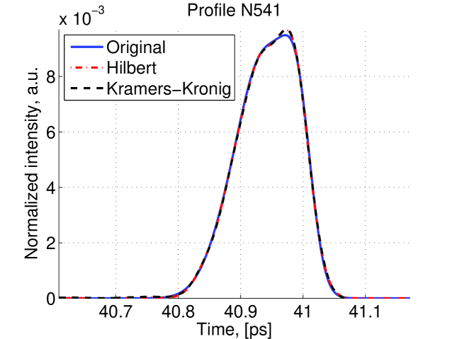
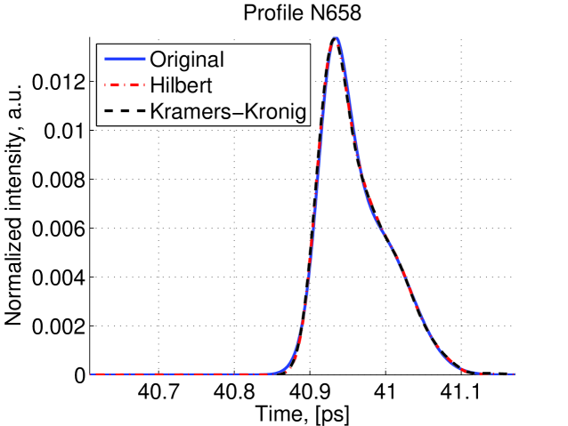
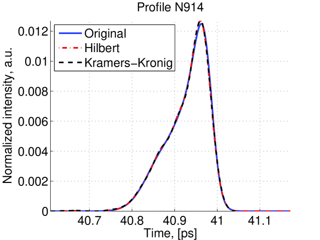
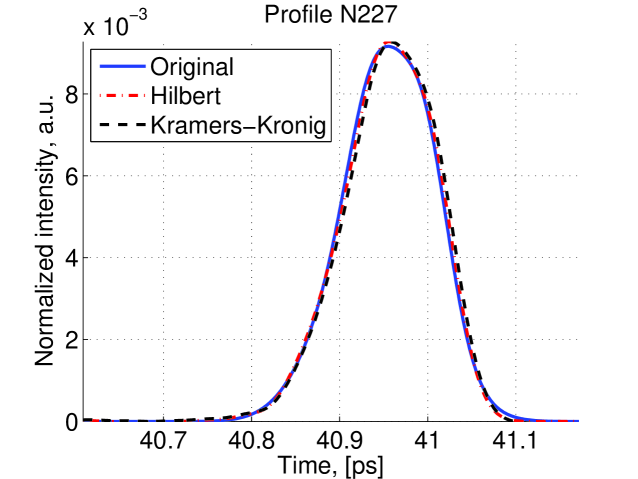
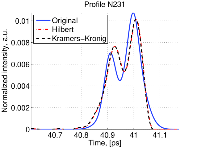
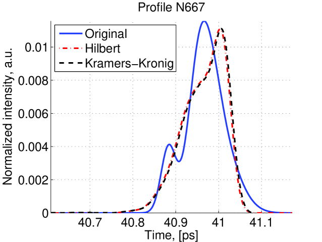
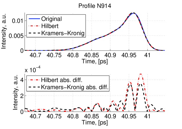
After applying extrapolation and interpolation, the spectrum recovery is completed. Then we used different reconstruction techniques to reconstruct the original profile. For each reconstruction method some profiles are very well reconstructed whereas some other are not so well reconstructed. Examples of well reconstructed profiles are shown in figure 11 and examples of poorly reconstructed profile are shown in figure 12.
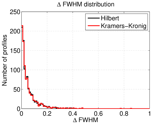
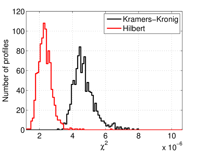
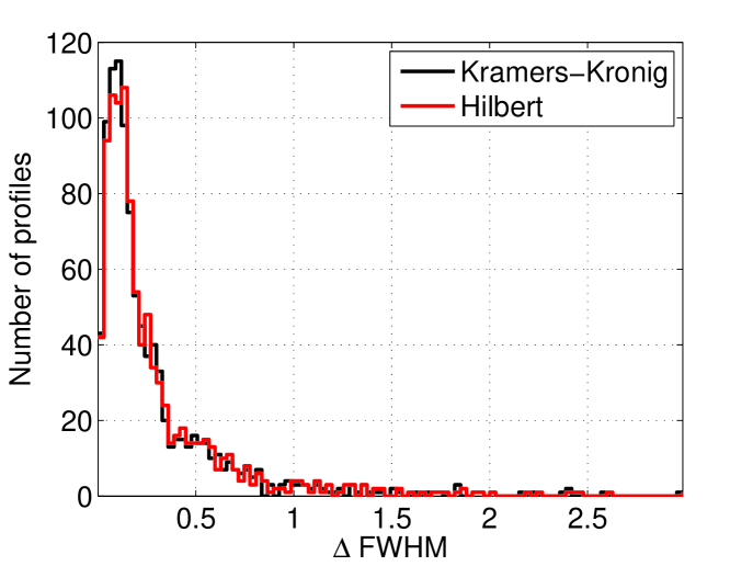
The and distribution of the 1000 simulations which were made and then reconstructed using the Hilbert transform method and Kramers-Kornig reconstruction are shown in figure 13. There is a good concordance in FWHM between two methods indicating that they are both good at finding the bunch length. However, the Hilbert method gives lower indicating that this method is better at reconstruction of the bunch profile.
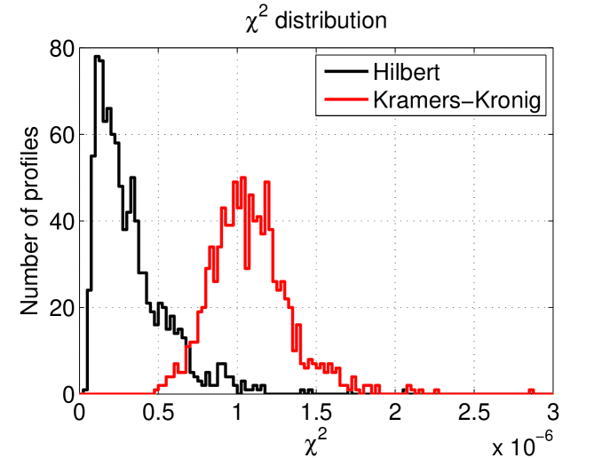
The fact that the phase recovery method based on the Kramers-Kronig relation gives a worst than the method based on Hilbert relation has been investigated. It is caused by the presence of negative components in the tails of the profiles. Figure 14 highlights this issue for one of the profiles.
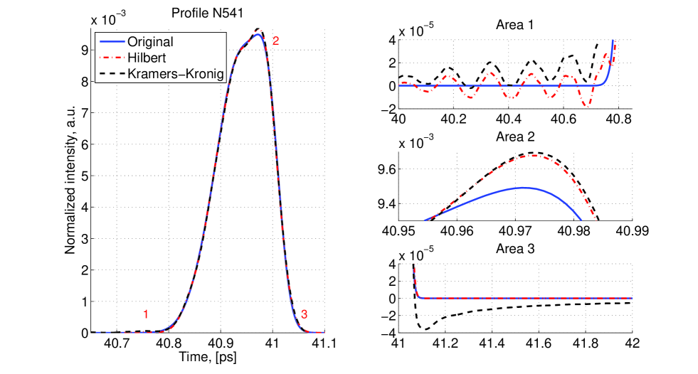
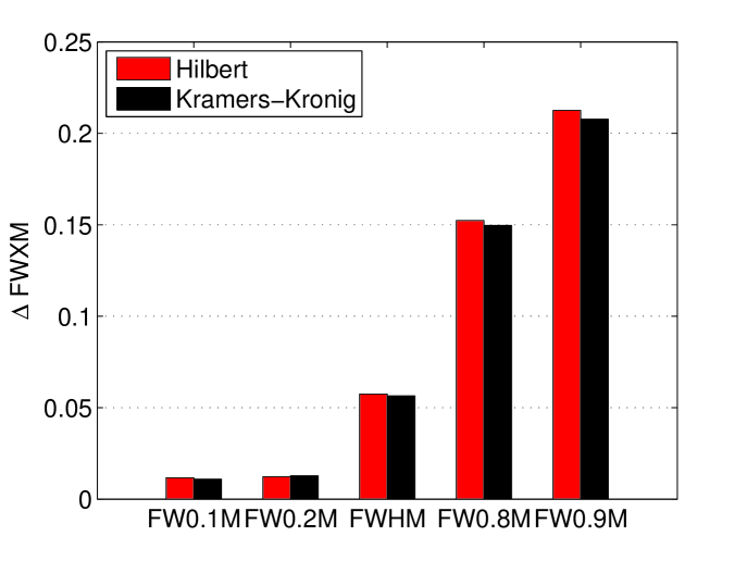
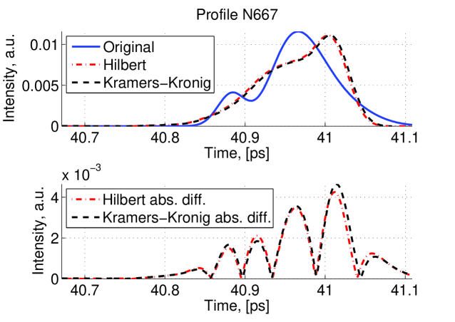
Figure 15 shows the different FWXH values for different values of X. This shows that at different height of the profiles the quality of reconstruction varies: there is a better agreement in the tails (X=10%) than at the top of the profile (X=90%). Figure 16 shows the modulus of the difference between the original and reconstructed profiles. One can see oscillations in the difference between the original and reconstructed profile.
While doing this work we also became aware of the discussion in [6] where it is argued that these reconstruction method have more difficulties with lorentzian profiles than gaussian profiles. Therefore we simulated 1000 Lorenzian profiles and performed a similar study. This is shown in figure 17. Although the is slightly worse in that case than in the case of gaussian profiles there still a good agreement between the original and reconstructed profiles.
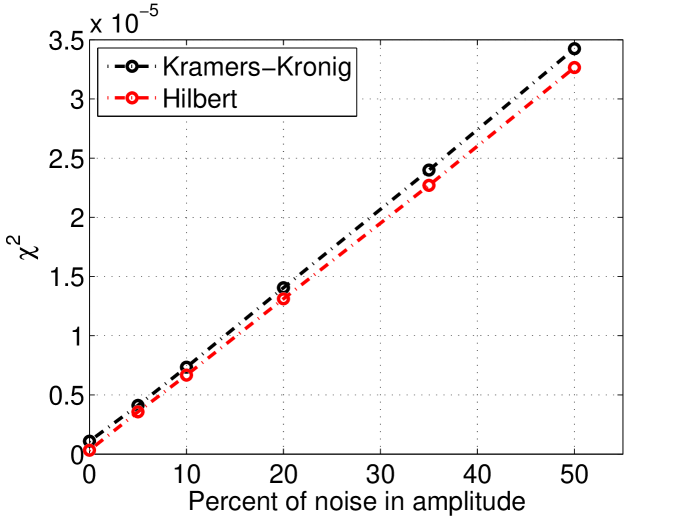
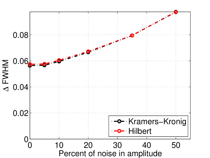
In our discussion so far we considered only the ideal case where no noise is added to the measured spectrum. However in a real experiment a noise component has to be added to the measured spectrum. This noise was added as follow :
| (17) |
where is the observed value, is the observed value with noise, is a random number between 0 and 1 (all numbers between 0 and 1 being equiprobable), and is the maximum noise for that simulation (depending on the case this can be 5%, 10%, 20%, 30%, 40% or 50%). This study was done using linear sampling with 33 samples and 1000 simulated profiles for each noise value. Figure 18 shows how the is modified when this noise component is added.
5 Discussion
We performed extensive simulation to estimate the performance of two phase recovery methods in the case of multi-gaussian and Lorenzian profiles. In both cases we found that when the sampling frequencies are chosen correctly we obtained a good agreement between the original and reconstructed profiles (in most cases ; ). This confirms that such methods are suitable to reconstruct the longitudinal profiles measured at particle accelerators using radiative methods.
The authors are grateful for the funding received from the French ANR (contract ANR-12-JS05-0003-01), the PICS (CNRS) "Development of the instrumentation for accelerator experiments, beam monitoring and other applications" and Research Grant #F58/380-2013 (project F58/04) from the State Fund for Fundamental Researches of Ukraine in the frame of the State key laboratory of high energy physics and the IDEATE International Associated Laboratory (LIA).
References
- [1] M.-A Tordeux and J. Papadacci. A new OTR based beam emittance monitor for the linac of LURE. EPAC 2000.
- [2] A. Cianchi, et al. Non-intercepting diagnostic for high brightness electron beams using optical diffraction radiation interference (odri). Journal of Physics: Conference Series, 357(1):012019, 2012.
- [3] V. Blackmore et al. First measurements of the longitudinal bunch profile of a 28.5 GeV beam using coherent Smith-Purcell radiation. Phys. Rev. ST Accel. Beams, 12:032803, Mar 2009.
- [4] O. Grimm and P. Schmüser. Principles of longitudinal beam diagnostics with coherent radiation. TESLA FEL note, page 03, 2006.
- [5] L. Andrews et al. Reconstruction of the time profile of 20.35 GeV, subpicosecond long electron bunches by means of Coherent Smith-Purcell radiation. Phys. Rev. ST Accel. Beams, 17:052802, May 2014.
- [6] Daniele Pelliccia and Tanaji Sen. A two-step method for retrieving the longitudinal profile of an electron bunch from its coherent radiation. 2014.
- [7] Victoria Blackmore. Determination of the Time Profile of Picosecond-Long Electron Bunches through the use of Coherent Smith-Purcell Radiation. 2008.
- [8] MATLAB documentation http://fr.mathworks.com/help /matlab/ref/pchip.html
- [9] R. Lai, U. Happek and A. J. Sievers Measurement of the Longitudinal Asymmetry of a Charged Particle Bunch from the Coherent Synchrotron or Transition Radiation Spectrum Phys. Rev. E, Vol. 50, No. 6, R4294 1994
- [10] Lars Frohlich Bunch Length Measurements Using a Martin-Puplett Interferometer at the VUV-FEL. 2005.