Study of Robust Adaptive Power Allocation Techniques for Rate Splitting based MU-MIMO systems
Abstract
Rate splitting (RS) systems can better deal with imperfect channel state information at the transmitter (CSIT) than conventional approaches. However, this requires an appropriate power allocation that often has a high computational complexity, which might be inadequate for practical and large systems. To this end, adaptive power allocation techniques can provide good performance with low computational cost. This work presents novel robust and adaptive power allocation technique for RS-based multiuser multiple-input multiple-output (MU-MIMO) systems. In particular, we develop a robust adaptive power allocation based on stochastic gradient learning and the minimization of the mean-square error between the transmitted symbols of the RS system and the received signal. The proposed robust power allocation strategy incorporates knowledge of the variance of the channel errors to deal with imperfect CSIT and adjust power levels in the presence of uncertainty. An analysis of the convexity and stability of the proposed power allocation algorithms is provided, together with a study of their computational complexity and theoretical bounds relating the power allocation strategies. Numerical results show that the sum-rate of an RS system with adaptive power allocation outperforms RS and conventional MU-MIMO systems under imperfect CSIT.
Index Terms:
Rate splitting, multiuser MIMO, power allocation, ergodic sum rate.I Introduction
Wireless communications systems employing multiple antennas have the advantage of increasing the overall throughput without increasing the required bandwidth. For this reason, multiple-antenna systems are at the core of several wireless communications standards such as WiFi, Long Term Evolution (LTE) and the fifth generation (5G). However, such wireless systems suffer from multiuser interference (MUI). In order to mitigate MUI, transmit processing techniques have been employed in the downlink (DL), allowing accurate recovery of the data at the receivers. In general, a precoding technique maps the symbols containing the information to the transmit antennas so that the information arrives at the receiver with reduced levels of MUI. Due to its benefits, linear [1, 2, 3, 4, 5, 6] and non-linear [7, 8, 9] precoding techniques have been extensively reported in the literature. The design of effective precoders demands very accurate channel state information at the transmitter (CSIT), which is an extremely difficult task to accomplish in actual wireless systems. Hence, the transmitter typically only has access to partial or imperfect CSIT. As a result, the precoder cannot handle MUI as expected, resulting in residual MUI at the receiver. This residual MUI can degrade heavily the performance of wireless systems since it scales with the transmit power employed at the base station (BS) [10].
I-A Prior and related work
In this context, Rate Splitting (RS) has emerged as a novel approach that is capable of dealing with CSIT imperfection [11] in an effective way. RS was initially proposed in [12] to deal with interference channels [13], where independent transmitters send information to independent receivers [14]. Since then, several studies have found that RS outperforms conventional schemes such as conventional precoding in spatial division multiple access (SDMA), power-domain Non-Orthogonal Multiple Access (NOMA) [15] and even dirty paper coding (DPC) [16]. Interestingly, it turns out that RS constitutes a generalized framework which has as special cases other transmission schemes such SDMA, NOMA and multicasting [17, 18, 19, 20]. The main advantage of RS is its capability to partially decode interference and partially treat interference as noise. To this end, RS splits the message of one or several users into a common message and a private message. The common message must be decoded by all the users that employ successive interference cancellation [21, 22, 23, 24, 25]. On the other hand, the private messages are decoded only by their corresponding users.
RS schemes have been shown to enhance the performance of wireless communication systems. In [26] RS was extended to the broadcast channel (BC) of multiple-input single-output (MISO) systems, where it was shown that RS provides gains in terms of Degrees-of-Freedom (DoF) with respect to conventional multiuser multiple-input multiple-output (MU-MIMO) schemes under imperfect CSIT. Later in [27], the DoF of a MIMO BC and IC was characterized. RS has eventually been shown in [28] to achieve the optimal DoF region when considering imperfect CSIT, outperforming the DoF obtained by SDMA systems, which decays in the presence of imperfect CSIT.
Due to its benefits, several wireless communications deployments with RS have been studied. RS has been employed in MISO systems along with linear precoders [29, 30] in order to maximize the sum-rate performance under perfect and imperfect CSIT assumptions. Another approach has been presented in [31] where the max-min fairness problem has been studied. In [32] a K-cell MISO IC has been considered and the scheme known as topological RS presented. The topological RS scheme transmits multiple layers of common messages, so that the common messages are not decoded by all users but by groups of users. RS has been employed along with random vector quantization in [33] to mitigate the effects of the imperfect CSIT caused by finite feedback. In [34, 35], RS with common stream combining techniques has been developed in order to exploit multiple antennas at the receiver and to improve the overall sum-rate performance. A successive null-space precoder, that employs null-space basis vectors to adjust the inter-user-interference at the receivers, is proposed in [36]. The optimization of the precoders along with the transmission of multiple common streams was considered in [37]. In [38], RS with joint decoding has been explored. The authors of [38] devised precoding algorithms for an arbitrary number of users along with a stream selection strategy to reduce the number of precoded signals.
Along with the design of the precoders, power allocation is also a fundamental part of RS-based systems. The benefits of RS are obtained only if an appropriate power allocation for the common stream is performed. However, the power allocation problem in MU-MIMO systems is an NP-hard problem [39, 40], and the optimal solution can be found at the expense of an exponential growth in computational complexity. Therefore, suboptimal approaches that jointly optimize the precoder and the power allocation have been developed. Most works so far employ exhaustive search or complex optimization frameworks. These frameworks rely on the augmented WMMSE [16, 41, 42, 43, 37], which is an extension of the WMMSE proposed in [44]. This approach requires also an alternating optimization, which further increases the computational complexity. A simplified approach can be found in [45], where closed-form expressions for RS-based massive MIMO systems are derived. However, this suboptimal solution is more appropiate for massive MIMO deployments. The high complexity of most optimal approaches makes them impractical to implement in large or real-time systems. For this reason, there is a strong demand for cost-effective power allocation techniques for RS systems.
I-B Contributions
In this paper, we present novel efficient robust and adaptive power allocation techniques [46] for RS-based MU-MIMO systems. In particular, we develop a robust adaptive power allocation (APA-R) strategy based on stochastic gradient learning [47, 48, 49, 50] and the minimization of the mean-square error (MSE) between the transmitted common and private symbols of the RS system and the received signal. We incorporate knowledge of the variance of the channel errors to cope with imperfect CSIT and adjust power levels in the presence of uncertainty. When the knowledge of the variance of the channel errors is not exploited the proposed APA-R becomes the proposed adaptive power allocation algorithm (APA). An analysis of the convexity and stability of the proposed power allocation algorithms along with a study of their computational complexity and theoretical bounds relating the power allocation strategies are developed. Numerical results show that the sum-rate of an RS system employing adaptive power allocation outperforms conventional MU-MIMO systems under imperfect CSIT assumption. The contributions of this work can be summarized as:
-
•
Cost-effective APA-R and APA techniques for power allocation are proposed based on stochastic gradient recursions and knowledge of the variance of the channel errors for RS-based and standard MU-MIMO systems.
-
•
An analysis of convexity and stability of the proposed power allocation techniques along with a bound on the MSE of APA and APA-R and a study of their computational complexity.
-
•
A simulation study of the proposed APA and APA-R, and the existing power allocation techniques for RS-based and standard MU-MIMO systems.
I-C Organization
The rest of this paper is organized as follows. Section II describes the mathematical model of an RS-based MU-MIMO system. In Section III the proposed APA-R technique is presented, the proposed APA approach is obtained as a particular case and sum-rate expressions are derived. In Section IV, we present an analysis of convexity and stability of the proposed APA and APA-R techniques along with a bound on the MSE of APA and APA-R and a study of their computational complexity. Simulation results are illustrated and discussed in Section V. Finally, Section VI presents the conclusions of this work.
I-D Notation
Column vectors are denoted by lowercase boldface letters. The vector stands for the th row of matrix . Matrices are denoted by uppercase boldface letters. Scalars are denoted by standard letters. The superscript represents the transpose of a matrix, whereas the notation stands for the conjugate transpose of a matrix. The operators , and represent the Euclidean norm, and the expectation w.r.t the random variable , respectively. The trace operator is given by . The Hadamard product is denoted by . The operator produces a diagonal matrix with the coefficients of located in the main diagonal.
II System Model
Let us consider the RS-based MU-MIMO system architecture depicted in Fig. 1, where the BS is equipped with antennas, serves users and the th UE is equipped with antennas. Let us denote by the total number of receive antennas. Then, . For simplicity, the message intended for the th user is split into a common message and a private message. Then, the messages are encoded and modulated. The transmitter sends one common stream and a total of private streams, with . The set contains the private streams, that are intended for the user , where . It follows that .
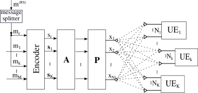
The vector , which is assumed i.i.d. with zero mean and covariance matrix equal to the identity matrix, contains the information transmitted to all users, where is the common symbol and contains the private symbols of all users. Specifically, the vector contains the private streams intended for the th user. The system is subject to a transmit power constraint given by , where is the transmitted vector and denotes the total available power. The transmitted vector can be expressed as follows:
| (1) |
where represents the power allocation matrix and is used to precode the vector of symbols . Specifically, and , where denotes the power allocated to the common stream and allocates power to the th private stream. Without loss of generality, we assume that the columns of the precoders are normalized to have unit norm.
The model established leads us to the received signal described by
| (2) |
where represents the uncorrelated noise vector, which follows a complex normal distribution, i.e., . We assume that the noise and the symbols are uncorrelated, which is usually the case in real systems. The matrix denotes the channel between the BS and the user terminals. Specifically, denotes the noise affecting the th user and the matrix represents the channel between the BS and the th user. The imperfections in the channel estimate are modelled by the random matrix . Each coefficient of follows a Gaussian distribution with variance equal to and . Then, the channel matrix can be expressed as , where the channel estimate is given by . From (2) we can obtain the received signal of user , which is given by
| (3) |
Note that the RS architecture contains the conventional MU-MIMO as a special case where no message is split and therefore is set to zero. Then, the model boils down to the model of a conventional MU-MIMO system, where the received signal at the th user is given by
| (4) |
In what follows, we will focus on the development of power allocation techniques that can cost-effectively compute and .
III Proposed Power Allocation Techniques
In this section, we detail the proposed power allocation techniques. In particular, we start with the derivation of the ARA-R approach and then present the APA technique as a particular case of the APA-R approach.
III-A Robust Adaptive Power Allocation
Here, a robust adaptive power allocation algorithm, denoted as APA-R, is developed to perform power allocation in the presence of imperfect CSIT. The key idea is to incorporate knowledge about the variance of the channel uncertainty [51, 52] into an adaptive recursion to allocate the power among the streams. The minimization of the MSE between the received signal and the transmitted symbols is adopted as the criterion to derive the algorithm.
Let us consider the model established in (2) and denote the fraction of power allocated to the common stream by the parameter , i.e., . It follows that the available power for the private streams is reduced to . We remark that the length of is greater than that of since the common symbol is superimposed to the private symbols. Therefore, we consider the vector , where is a transformation matrix employed to ensure that the dimensions of and match, and is given by
| (5) |
All the elements in the first row of matrix are equal to one in order to take into account the common symbol obtained at all receivers. As a result we obtain the combined receive signal of all users. It follows that
| (6) |
where the received signal at the th antenna is described by
| (7) |
Let us now consider the proposed robust power allocation problem for imperfect CSIT scenarios. By including the error of the channel estimate, the robust power allocation problem can be formulated as the constrained optimization given by
| (8) |
which can be solved by first relaxing the constraint, using an adaptive learning recursion and then enforcing the constraint.
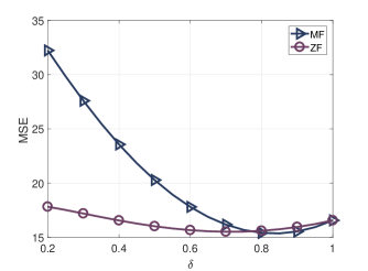
In this work, we choose the MSE as the objective function due to its convex property and mathematical tractability, which help to find an appropriate solution through algorithms. The objective function is convex as illustrated by Fig. 2 and analytically shown in Section IV. In Fig. 2, we plot the objective function using two precoders, namely the zero-forcing (ZF) and the matched filter (MF) precoders [2], where three private streams and one common stream are transmitted and the parameter varies with uniform power allocation across private streams.
To solve (8) we need to expand the terms and evaluate the expected value. Let us consider that the square error is equal to . Then, the MSE is given by
| (9) |
where and for all . The proof to obtain the last equation can be found in appendix A. The partial derivatives of (9) with respect to and are expressed by
| (10) |
| (11) |
The partial derivatives given by (10) and (11) represent the gradient of the MSE with respect to the power allocation coefficients. With the obtained gradient we can employ a gradient descent algorithm, which is an iterative procedure that finds a local minimum of a differentiable function. The key idea is to take small steps in the opposite direction of the gradient, since this is the direction of the steepest descent. Remark that the objective function used is convex and has no local minimum. Then, the recursions of the proposed APA-R technique are given by
| (12) |
where the parameter represents the learning rate of the adaptive algorithm. At each iteration, the power constraint is analyzed. Then, the coefficients are scaled with a power scaling factor by , where to ensure that the power constraint is satisfied. Algorithm 1 summarizes the proposed APA-R algorithm.
III-B Adaptive Power Allocation
In this section, a simplified version of the proposed APA-R algorithm is derived. The main objective is to reduce the complexity of each recursion of the adaptive algorithm and avoid the load of computing the statistical parameters of the imperfect CSIT, while reaping the benefits of RS systems. The power allocation problem can be reformulated as the constrained optimization problem given by
| (13) |
In this case, the MSE is equivalent to
| (14) |
where we considered that and for all . The proof to obtain (14) can be found in appendix B. Taking the partial derivatives of (14) with respect to the coefficients of we arrive at
| (15) | ||||
| (16) |
The power allocation coefficients are adapted using (15) and (16) in the following recursions:
| (17) |
III-C Sum-Rate Performance
In this section, we derive closed-form expressions to compute the sum-rate performance of the proposed algorithms. Specifically, we employ the ergodic sum-rate (ESR) as the main performance metric. Before the computation of the ESR we need to find the average power of the received signal, which is given by
| (18) |
It follows that the instantaneous SINR while decoding the common symbol is given by
| (19) |
Once the common symbol is decoded, we apply SIC to remove it from the received signal. Afterwards, we calculate the instantaneous SINR when decoding the th private stream, which is given by
| (20) |
Considering Gaussian signaling, the instantaneous common rate can be found with the following equation:
| (21) |
The private rate of the th stream is given by
| (22) |
Since imperfect CSIT is being considered, the instantaneous rates are not achievable. To that end, we employ the average sum rate (ASR) to average out the effect of the error in the channel estimate. The average common rate and the average private rate are given by
| (23) |
respectively. With the ASR we can obtain the ergodic sum-rate (ESR), which quantifies the performance of the system over a large number of channel realizations and is given by
| (24) |
IV Analysis
In this section, we carry out a convexity analysis and a statistical analysis of the proposed algorithms along with an assessment of their computational complexity in terms of floating point operations (FLOPs). Moreover, we derive a bound that establishes that the proposed APA-R algorithm is superior or comparable to the proposed APA algorithm.
IV-A Convexity analysis
In this section, we perform a convexity analysis of the optimization problem that gives rise to the proposed APA-R and APA algorithms. In order to establish convexity, we need to compute the second derivative of with respect to and , and then check if it is greater than zero [47], i.e.,
| (25) |
Let us first compute using the results in (10):
| (26) |
Now let us compute using the results in (11):
| (27) |
Since we have the sum of the strictly convex terms in (26) and (27) the objective function associated with APA-R is strictly convex [47]. The power constraint is also strictly convex and only scales the powers to be adjusted. In the case of the APA algorithm, the objective function does not employ knowledge of the error variance and remains strictly convex.
IV-B Bound on the MSE of APA and APA-R
Let us now show that the proposed APA-R power allocation produces a lower MSE than that of the proposed APA power allocation. The MSE obtained in (14) assumes that the transmitter has perfect knowledge of the channel. Under such assumption the optimal coefficients that minimize the error are found. However, under imperfect CSIT the transmitter is unaware of and the adaptive algorithm performs the power allocation by employing instead of . This results in a power allocation given by which originates an increase in the MSE obtained. It follows that
| (28) |
On the other hand, the robust adaptive algorithm finds the optimal that minimizes and therefore takes into account that only partial knowledge of the channel is available. Since the coefficients and are different, we have
| (29) |
Note that under perfect CSIT equation (9) reduces to (14). In such circumstances and therefore both algorithms are equivalent. In the following, we evaluate the performance obtained by the proposed algorithms. Specifically, we have that , where is the error produced from the assumption that the BS has perfect CSIT. Then, we have
| (30) |
which is a positive quantity when and . The inequalities hold as long as and . As the error in the power allocation coefficients grows the left-hand side of the two last inequalities increases. This explains why the proposed APA-R performs better than the proposed APA algorithm.
IV-C Statistical Analysis
The performance of adaptive learning algorithms is usually measured in terms of its transient behavior and steady-state behaviour. These measurements provide information about the stability, the convergence rate, and the MSE achieved by the algorithm[53, 54]. Let us consider the adaptive power allocation with the update equations given by (17). Expanding the terms of (17) for the private streams, we get
| (31) |
Let us define the error between the estimate of the power coefficients and the optimal parameters as follows:
| (32) |
where represents the optimal allocation for the th coefficient.
By subtracting (32) from (31), we obtain
| (33) |
where . Expanding the terms in (33), we get
Rearranging the terms of the last equation, we obtain
| (34) |
Equation (34) can be rewritten as follows
| (35) |
where
| (36) |
Bu multiplying (35) by and taking the expected value, we obtain
| (37) |
where we consider that .The previous equation constitutes a geometric series with geometric ratio equal to . Then, we have
| (38) |
Note that from the last equation the step size must fulfill
| (39) |
with .
For the common power allocation coefficient we have the following recursion:
| (40) |
where . The error with respect to the optimal power allocation of the common stream is given by
| (41) |
Following a similar procedure to the one employed for the private streams we arrive at
| (42) |
Multiplying the previous equation by and taking the expected value leads us to:
| (43) |
It follows that the geometric ratio of the recursion is equal to . Then, the step size must be in the following range:
| (44) |
where
| (45) |
The step-size of the algorithm must be less or equal to . The stability bounds provide useful information on the choice of the step sizes.
Let us now consider the APA-R algorithm. The a posteriori error can be expressed as follows:
| (46) |
Expanding the terms of the last equation, we get
| (47) |
The geometric ratio of the robust APA algorithm is given by . Then, we have that
| (48) |
Therefore, the step size must satisfy the following inequality:
| (49) |
where . Following a similar procedure for the power coefficient of the common stream lead us to
| (50) |
where
| (51) |
As in the previous case, the step size is chosen using . The variable has an additional term given by when compared to of the APA algorithm. In this sense, the upper bound of (70) is smaller than the bound in (65). In other words, the step size of APA-R takes smaller values than the step size of APA.
IV-D Computational Complexity
In this section the number of FLOPs performed by the proposed algorithms is computed. For this purpose let us consider the following results to simplify the analysis. Consider the complex vector and . Then, we have the following results:
-
•
The product requires FLOPs.
-
•
The term requires FLOPs
The gradient in equation (16) requires the computation of three terms. The first term, which is given by needs a total of FLOPs. The evaluation of the second term results in . For the last term we have a total of . Considering a system where we have that the number of FLOPs required by the proposed adaptive algorithm is given by .
The computational complexity of the gradients in (10) and (11) can be computed in a similar manner. However, in this case we have an additional term given by , which requires a total of FLOPs. Then, the robust adaptive algorithm requires a total of . It is important to mention that the computational complexity presented above represents the number of FLOPs of the adaptive algorithm per iteration.
In contrast, the optimal power allocation for the conventional SDMA system requires the exhaustive search over with a fine grid. Given a system with streams and a grid step of , the exhaustive search would require the evaluation of different power allocation matrices for each channel realization. In contrast, the adaptive approaches presented require only the computation of around iterations. Furthermore, the complexity of the exhaustive search for an RS system is even higher since the search is perform over , which additionally contains the power allocated to the common stream.
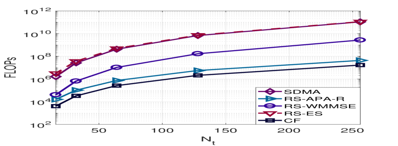
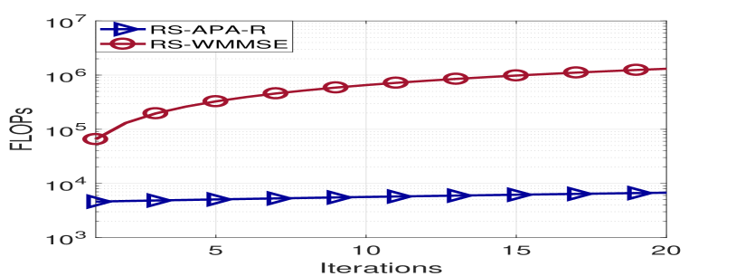
Table LABEL:Computational_complexity_power_allocation summarizes the computational complexity of the proposed algorithms employing the big notation. In Table LABEL:Computational_complexity_power_allocation, denotes the number of points of the grid given a step size, refers to the number of iterations of the alternating procedure and denotes the number of iterations for the adaptive algorithms. It is worth noting that . Moreover, the inner iterations employed in the WMMSE approach are much more demanding than the iterations of the proposed APA and APA-R algorithms. Fig 3(a) shows the computational complexity in terms of FLOPS assuming that the number of transmit antennas increases. The term CF represents the closed-form power allocation in [45], which requires the inversion of an matrix. The step of the grid was set to for the ES and the number of iterations to for the WMMSE, APA and APA-R approaches. Note that in practice the WMMSE iterates continuously until meeting a predefined accuracy. In general, it requires more than iterations. It is also important to point out that the cost per iteration of the adaptive approaches can be reduced after the first iteration. The precoders and the channel are fixed given a transmission block. Therefore, after the first iteration, we can avoid the multiplication of the precoder by the channel matrix in the update equation. In contrast, the WMMSE must perform the whole procedure again since the precoders are updated between iterations. This is illustrated in Fig. 3(b).
| Technique | |
|---|---|
| SDMA-ES | |
| WMMSE | |
| RS-ES | |
| RS-APA | |
| RS-APA-R | |
| CF[45] |
.
V Simulations
In this section, the performance of the proposed APA-R and APA algorithms is assessed against existing power allocation approaches, namely, the ES, the WMMSE [42], the closed-form approach of [45], the power allocation obtained directly from the precoders definition which is denoted here as random power allocation, and the uniform power allocation (UPA) approaches. Unless otherwise specified, we consider an RS MU-MIMO system where the BS is equipped with four antennas and transmits data to two users, each one equipped with two antennas. The inputs are statistically independent and follow a Gaussian distribution. A flat fading Rayleigh channel, which remains fixed during the transmission of a packet, is considered, we assume additive white Gaussian noise with zero mean and unit variance, and the SNR varies with . For all the experiments, the common precoder is computed by employing a SVD over the channel matrix, i.e. . Then we set the common precoder equal to the first column of matrix , i.e., .
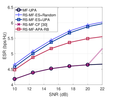
In the first example, we consider the transmission under imperfect CSIT. The proposed APA-R algorithm is compared against the closed form expression from [45] and against ES with random and UPA algorithms. The first ES approach fixes a random power allocation for the private streams and then an exhaustive search is carried out to find the best power allocation for the common stream. The second scheme considers that the power is uniformly distributed among private streams and then performs an exhaustive search to find the optimum value for . Fig. 4 shows the performance obtained with a MF. Although ES obtains the best performance, it requires a great amount of resources in terms of computational complexity. Moreover, we can see that the closed-form power allocation does not allocate power to the common message in the low SNR regime. The reason for this behavior is that this power allocation scheme was derived for massive MIMO environments where the excess of transmit antennas gets rid of the residual interference at low SNR and no common message is required. As the SNR increases the residual interference becomes larger and the algorithm allocates power to the common stream.
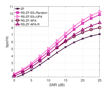
In the next example, the ZF precoder has been considered. The results illustrated in Fig. 5 show that the techniques that perform ES, which are termed as RS-ZF-ES+Random and RS-ZF-ES-UPA, have the best performance. However, the APA and APA-R adaptive algorithms obtain a consistent gain when compared to the conventional ZF algorithm.
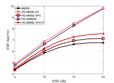
In Fig. 6 we employed the MMSE precoder. In this case, an exhaustive search was performed to obtain the best power allocation coefficients for all streams. The technique from [27] was also considered and is denoted in the figure as RS-WMMSE. We can observe that the best performance is obtained by ES. The proposed APA and APA-R algorithms obtain a consistent gain when compared to the conventional MMSE precoder. The performance is worse than that of ES and the RS-WMMSE, but the computational complexity is also much lower.
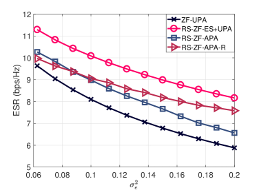
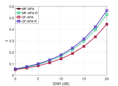
In the next example, we evaluate the performance of the proposed APA and APA-R techniques as the error in the channel estimate becomes larger. For this scenario, we consider a fixed SNR equal to 20 dB. Fig. 7 depicts the results of different power allocation techniques. The results show that the APA-R performs better than the APA as the variance of the error increases.
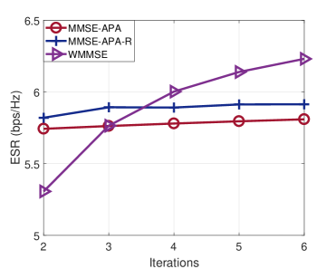
Let us now consider the ESR obtained versus the number of iterations, which is shown in Fig. 8. The step size of the adaptive algorithms was set to and the SNR to dB. Fig. 8 shows that APA and APA-R obtain better performance than WMMSE with few iterations, i.e., with reduced cost. Recall that the cost per iteration is much lower for the adaptive algorithms.
In Fig. 9 we can notice the power allocated to the common stream. For this simulation we consider the same setup as in the previous simulation. We can observe that the parameter increases with the SNR. In other words, as the MUI becomes more significant, more power is allocated to the common stream. We can also notice that the proposed APA-R algorithm allocates more power to the common stream than that of the APA algorithm.
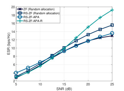
In the last example, we consider the ZF precoder in a MU-MIMO system where the BS is equipped with transmit antennas. The information is sent to users which are randomly distributed over the area of interest. Fig. 10 shows the results obtained by employing the proposed APA and APA-R algorithms. Specifically, it can be noticed that the RS system equipped with APA-R can obtain a gain of up to over that random allocation and up to over that of a conventional MU-MIMO system with random allocation.
VI Conclusion
In this work, adaptive power allocation techniques have been developed for RS-MIMO and conventional MU-MIMO systems. Differently to optimal and WMMSE power allocation often employed for RS-based systems that are computationally very costly, the proposed APA and APA-R algorithms have low computational complexity and require fewer iterations for new transmission blocks, being suitable for practical systems. Numerical results have shown that the proposed power allocation algorithms, namely APA and APA-R, are not very far from the performance of exhaustive search with uniform power allocation. Furthermore, the proposed robust technique, i.e., APA-R, increases the robustness of the system against CSIT imperfections.
Appendix A Proof of the MSE for the APA-R
In what follows the derivation of the MSE for the APA-R algorithm is detailed. Let us first expand the MSE, which is given by
| (52) |
The first term of (52) is independent from and can be reduced to the following expression:
| (53) |
The second term given by requires the computation of the following term:
| (54) |
By evaluating the expected value of the different terms in (54) we get the following quantities:
| (55) | ||||
| (56) |
where and . These expressions allow us to compute , which is expressed by
| (57) |
The third term can be calculated in a similar manner and is given by
| (58) |
The last term of equation (52) requires the computation of several quantities. Let us first consider the following quantity:
| (59) |
Taking the expected value on the last equation results in
| (60) |
| (61) |
where and . Expanding the terms of the last equation results in
| (62) |
Since the entries of are uncorrelated with zero mean and also independent from , we have
| (63) |
Note that and are independent from . Thus, we get
| (64) |
and similarly Then, (63) turns into
| (65) |
Let us now evaluate the expected value of when , which results in
| (66) |
Remark that and are independent with zero mean. Thus, the last equation is reduced to
| (67) |
Equations (65) allow us to compute the second term of equation (60), which is given by
| (68) |
On the other hand, (67) allow us to obtain the first term of (60), which results in
| (69) |
Applying the property , we can simplify half of the sums from the triple summation, i.e.,
| (70) |
It follows that
| (71) |
By using (68) and (71) in (60) and then substituting (53) (57), (58), and (60) in (52) we can calculate the MSE, which is given by (9). This concludes the proof.
Appendix B Proof of the MSE for the APA
Here, we describe in detail how to obtain the MSE employed in the APA algorithm. Let us first consider the MSE, which is given by
| (72) |
By taking the expected value of the second term in (72) and expanding the equation, we have
| (73) |
Since the symbols are uncorrelated, equation (73) is reduced to
| (74) |
The third term of (72) can be computed in a similar way as the second term, which lead us to
| (75) |
The last term of (72) is equal to
| (76) |
Let us first compute the quantity given by
| (77) |
Additionally, we know that
| (78) |
for all . From the last equation, we have
| (79) |
where we define and for all . Applying the property , we can simplify half of the sums from the triple summation, i.e.,
| (80) |
The final step to obtain the last term of (72) is to employ (77), (79), and (80) to compute the following quantities:
| (81) |
| (82) |
References
- [1] R. C. de Lamare, “Massive mimo systems: Signal processing challenges and future trends,” URSI Radio Science Bulletin, vol. 2013, no. 347, pp. 8–20, 2013.
- [2] M. Joham, W. Utschick, and J. A. Nossek, “Linear transmit processing in MIMO communications systems,” IEEE Transactions on Signal Processing, vol. 53, no. 8, pp. 2700–2712, Aug. 2005.
- [3] W. Zhang, H. Ren, C. Pan, M. Chen, R. C. de Lamare, B. Du, and J. Dai, “Large-scale antenna systems with ul/dl hardware mismatch: Achievable rates analysis and calibration,” IEEE Transactions on Communications, vol. 63, no. 4, pp. 1216–1229, 2015.
- [4] K. Zu, R. C. de Lamare, and M. Haardt, “Generalized design of low-complexity block diagonalization type precoding algorithms for multiuser mimo systems,” IEEE Transactions on Communications, vol. 61, no. 10, pp. 4232–4242, 2013.
- [5] W. Zhang, R. C. de Lamare, C. Pan, M. Chen, J. Dai, B. Wu, and X. Bao, “Widely linear precoding for large-scale mimo with iqi: Algorithms and performance analysis,” IEEE Transactions on Wireless Communications, vol. 16, no. 5, pp. 3298–3312, 2017.
- [6] Y. Cai, R. C. de Lamare, L.-L. Yang, and M. Zhao, “Robust mmse precoding based on switched relaying and side information for multiuser mimo relay systems,” IEEE Transactions on Vehicular Technology, vol. 64, no. 12, pp. 5677–5687, 2015.
- [7] K. Zu, R. C. de Lamare, and M. Haardt, “Multi-branch Tomlinson-Harashima precoding design for MU-MIMO systems: Theory and algorithms,” IEEE Transactions on Communications, vol. 62, no. 3, pp. 939–951, Mar. 2014.
- [8] C. Peel, B. Hochwald, and A. Swindlehurst, “A vector-perturbation technique for near-capacity multiantenna multiuser communication— part II: Perturbation,” IEEE Transactions on Communications, vol. 53, no. 1, pp. 537–544, Mar. 2005.
- [9] L. T. N. Landau and R. C. de Lamare, “Branch-and-bound precoding for multiuser mimo systems with 1-bit quantization,” IEEE Wireless Communications Letters, vol. 6, no. 6, pp. 770–773, 2017.
- [10] D. Tse and P. Viswanath, Fundamentals of Wireless Communications. Cambridge University Press, 2005.
- [11] B. Clerckx, H. Joudeh, C. Hao, M. Dai, and B. Rassouli, “Rate splitting for MIMO wireless networks: a promising PHY-layer strategy for LTE evolution,” IEEE Communications Magazine, vol. 54, no. 5, pp. 98–105, May 2016.
- [12] T. S. Han and K. Kobayashi, “A new achievable rate region for the interference channel,” IEEE Transactions on Information Theory, vol. 27, no. 1, pp. 49–60, Jan. 1981.
- [13] A. Carleial, “Interference channels,” IEEE Transactions on Information Theory, vol. 24, no. 1, pp. 60–70, Jan. 1978.
- [14] A. Haghi and A. K. Khandani, “Rate splitting and successive decoding for gaussian interference channels,” IEEE Transactions on Information Theory, vol. 67, no. 3, pp. 1699–1731, 2021.
- [15] Y. Mao, “Rate-splitting multiple access for downlink communications systems,” Ph.D. dissertation, The University of Hong Kong, 2018.
- [16] Y. Mao and B. Clerckx, “Beyond dirty paper coding for multi-antenna broadcast channel with partial CSIT: A rate-splitting approach,” IEEE Transactions on Communications, vol. 68, no. 11, pp. 6775–6791, Nov. 2020.
- [17] B. Clerckx, Y. Mao, R. Schober, and H. V. Poor, “Rate-splitting unifying SDMA, OMA, NOMA, and multicasting in MISO broadcast channel: A simple two-user rate analysis,” IEEE Wireless Communications Letters, vol. 9, no. 3, pp. 349–353, Mar. 2020.
- [18] S. Naser, P. C. Sofotasios, L. Bariah, W. Jaafar, S. Muhaidat, M. Al-Qutayri, and O. A. Dobre, “Rate-splitting multiple access: Unifying NOMA and SDMA in MISO VLC channels,” IEEE Open Journal of Vehicular Technology, vol. 1, pp. 393–413, Oct. 2020.
- [19] W. Jaafar, S. Naser, S. Muhaidat, P. C. Sofotasios, and H. Yanikomeroglu, “Multiple access in aerial networks: From orthogonal and non-orthogonal to rate-splitting,” IEEE Open Journal of Vehicular Technology, vol. 1, pp. 372–392, 2020.
- [20] Y. Mao, O. Dizdar, B. Clerckx, R. Schober, P. Popovski, and H. V. Poor, “Rate-splitting multiple access: Fundamentals, survey, and future research trends,” arXiv:2201.03192v1 [cs.IT], Jan. 2022.
- [21] R. C. De Lamare and R. Sampaio-Neto, “Minimum mean-squared error iterative successive parallel arbitrated decision feedback detectors for ds-cdma systems,” IEEE Transactions on Communications, vol. 56, no. 5, pp. 778–789, 2008.
- [22] P. Li, R. C. de Lamare, and R. Fa, “Multiple feedback successive interference cancellation detection for multiuser mimo systems,” IEEE Transactions on Wireless Communications, vol. 10, no. 8, pp. 2434–2439, 2011.
- [23] R. C. de Lamare, “Adaptive and iterative multi-branch mmse decision feedback detection algorithms for multi-antenna systems,” IEEE Transactions on Wireless Communications, vol. 12, no. 10, pp. 5294–5308, 2013.
- [24] A. G. D. Uchoa, C. T. Healy, and R. C. de Lamare, “Iterative detection and decoding algorithms for mimo systems in block-fading channels using ldpc codes,” IEEE Transactions on Vehicular Technology, vol. 65, no. 4, pp. 2735–2741, 2016.
- [25] Z. Shao, R. C. de Lamare, and L. T. N. Landau, “Iterative detection and decoding for large-scale multiple-antenna systems with 1-bit adcs,” IEEE Wireless Communications Letters, vol. 7, no. 3, pp. 476–479, 2018.
- [26] S. Yang, M. Kobayashi, D. Gesbert, and X. Yi, “Degrees of freedom of time correlated MISO broadcast channel with delayed CSIT,” IEEE Transactions on Information Theory, vol. 59, no. 1, pp. 315–328, Jan. 2013.
- [27] C. Hao, B. Rassouli, and B. Clerckx, “Achievable dof regions of mimo networks with imperfect csit,” IEEE Transactions on Information Theory, vol. 63, no. 10, pp. 6587–6606, Oct 2017.
- [28] E. Piovano and B. Clerckx, “Optimal DoF region of the -user MISO BC with partial CSIT,” IEEE Communications Letters, vol. 21, no. 11, pp. 2368–2371, Nov. 2017.
- [29] H. Joudeh, “A rate-spliting approach to multiple-antenna broadcasting,” Ph.D. dissertation, Imperial College London, 2016.
- [30] C. Hao, Y. Wu, and B. Clerckx, “Rate analysis of two-receiver MISO broadcast channel with finite rate feedback: A rate-splitting approach,” IEEE Transactions on Communications, vol. 63, no. 9, pp. 3232–3246, Sep. 2015.
- [31] H. Joudeh and B. Clerckx, “Rate-splitting for max-min fair multigroup multicast beamforming in overloaded systems,” IEEE Transactions on Wireless Communications, vol. 16, no. 11, pp. 7276–7289, Nov. 2017.
- [32] C. Hao and B. Clerckx, “MISO networks with imperfect CSIT: A topological rate-splitting approach,” IEEE Transactions on CommunicationsIEEE Transactions on Communications, vol. 65, no. 5, pp. 2164–2179, May 2017.
- [33] G. Lu, L. Li, H. Tian, and F. Qian, “MMSE-based precoding for rate splitting systems with finite feedback,” IEEE Communications Letters, vol. 22, no. 3, pp. 642–645, Mar. 2018.
- [34] A. R. Flores, R. C. De Lamare, and B. Clerckx, “Linear precoding and stream combining for rate splitting in multiuser MIMO systems,” IEEE Communications Letters, vol. 24, no. 4, pp. 890–894, Jan. 2020.
- [35] A. R. Flores, R. C. De Lamare, and B. Clerckx, “Tomlinson-harashima precoded rate-splitting with stream combiners for MU-MIMO systems,” IEEE Transactions on Communications, pp. 1–1, 2021.
- [36] A. Krishnamoorthy and R. Schober, “Successive null-space precoder design for downlink MU-MIMO with rate splitting and single-stage SIC,” in 2021 IEEE International Conference on Communications Workshops (ICC Workshops), 2021, pp. 1–6.
- [37] A. Mishra, Y. Mao, O. Dizdar, and B. Clerckx, “Rate-splitting multiple access for downlink multiuser MIMO: Precoder optimization and PHY-layer design,” IEEE Transactions on Communications, vol. 70, no. 2, pp. 874–890, Feb. 2022.
- [38] Z. Li, C. Ye, Y. Cui, S. Yang, and S. Shamai, “Rate splitting for multi-antenna downlink: Precoder design and practical implementation,” IEEE Journal on Selected Areas in Communications, vol. 38, no. 8, pp. 1910–1924, 2020.
- [39] Z. Luo and S. Zhang, “Dynamic spectrum management: Complexity and duality,” IEEE Journal of Selected Topics in Signal Processing, vol. 2, no. 1, pp. 57–73, Feb. 2008.
- [40] Y. Liu, Y. Dai, and Z. Luo, “Coordinated beamforming for MISO interference channel: Complexity analysis and efficient algorithms,” IEEE Transactions on Signal Processing, vol. 59, no. 3, pp. 1142–1157, Mar. 2011.
- [41] Y. Mao, B. Clerckx, and V. Li, “Rate-splitting multiple access for downlink communication systems: Bridging, generalizing and outperforming SDMA and NOMA,” EURASIP Journal on Wireless Communications and Networking, vol. 2018, no. 1, p. 133, May 2018.
- [42] H. Joudeh and B. Clerckx, “Sum-rate maximization for linearly precoded downlink multiuser MISO systems with partial CSIT: A rate-splitting approach,” IEEE Transactions on Communications, vol. 64, no. 11, pp. 4847–4861, Nov. 2016.
- [43] C. Kaulich, M. Joham, and W. Utschick, “Rate-splitting for the weighted sum rate maximization under minimum rate constraints in the MIMO BC,” in 2021 IEEE International Conference on Communications Workshops (ICC Workshops), 2021, pp. 1–6.
- [44] S. S. Christensen, R. Agarwal, E. De Carvalho, and J. M. Cioffi, “Weighted sum-rate maximization using weighted MMSE for MIMO-BC beamforming design,” IEEE Transactions on Wireless Communications, vol. 7, no. 12, pp. 4792–4799, Dec. 2008.
- [45] M. Dai, B. Clerckx, D. Gesbert, and G. Caire, “A rate splitting strategy for massive mimo with imperfect csit,” IEEE Transactions on Wireless Communications, vol. 15, no. 7, pp. 4611–4624, Jul. 2016.
- [46] A. R. Flores and R. C. De Lamare, “Robust and adaptive power allocation techniques for rate splitting based mu-mimo systems,” IEEE Transactions on Communications, pp. 1–1, 2022.
- [47] D. P. Bertsekas, N. Angelia, and A. E. Ozdaglar, Convex Analysis and. Optimization. Athena Scientific, Belmont, MA:, 2003.
- [48] R. C. de Lamare and R. Sampaio-Neto, “Adaptive reduced-rank processing based on joint and iterative interpolation, decimation, and filtering,” IEEE Transactions on Signal Processing, vol. 57, no. 7, pp. 2503–2514, 2009.
- [49] R. C. de Lamare and P. S. R. Diniz, “Set-membership adaptive algorithms based on time-varying error bounds for cdma interference suppression,” IEEE Transactions on Vehicular Technology, vol. 58, no. 2, pp. 644–654, 2009.
- [50] T. Wang, R. C. de Lamare, and P. D. Mitchell, “Low-complexity set-membership channel estimation for cooperative wireless sensor networks,” IEEE Transactions on Vehicular Technology, vol. 60, no. 6, pp. 2594–2607, 2011.
- [51] H. Ruan and R. C. de Lamare, “Robust adaptive beamforming using a low-complexity shrinkage-based mismatch estimation algorithm,” IEEE Signal Processing Letters, vol. 21, no. 1, pp. 60–64, 2014.
- [52] ——, “Robust adaptive beamforming based on low-rank and cross-correlation techniques,” IEEE Transactions on Signal Processing, vol. 64, no. 15, pp. 3919–3932, 2016.
- [53] N. Yousef and A. Sayed, “A unified approach to the steady-state and tracking analyses of adaptive filters,” IEEE Transactions on Signal Processing, vol. 49, no. 2, pp. 314–324, 2001.
- [54] A. Sayed, Fundamentals of Adaptive Filtering. Fundamentals of Adaptive Filtering, 2003.