Department of Physics and Astrophysics \universityUniversity of Delhi \degreeDoctor of Philosophy \degreedateMay 2008
Study of the Structure and Dynamics of Complex Biological Networks
Declaration
This thesis describes work done by the candidate during his tenure as Ph.D. student at the Department of Physics and Astrophysics, University of Delhi, Delhi, India under the supervision of Prof. Sanjay Jain and Prof. Shobhit Mahajan. The work reported in this thesis is original and it has not been submitted earlier for any degree to any university.
Candidate:
Supervisor:
Supervisor:
Head of the Department:
List of Publications
In International Refereed Journals
-
1.
Low degree metabolites explain essential reactions and enhance modularity in biological networks,
Areejit Samal, Shalini Singh, Varun Giri, Sandeep Krishna, N. Raghuram and Sanjay Jain,
BMC Bioinformatics, 7:118 (2006). -
2.
The regulatory network of E. coli metabolism as a Boolean dynamical system exhibits both homeostasis and flexibility of response,
Areejit Samal and Sanjay Jain,
BMC Systems Biology, 2:21 (2008). -
3.
A universal power law and proportionate change process characterize the evolution of metabolic networks,
Shalini Singh, Areejit Samal, Varun Giri, Sandeep Krishna, N. Raghuram and Sanjay Jain,
Eur. Phys. J. B, 57:75-80 (2007).
The work reported in this thesis is based on publications 1 and 2 mentioned above.
In Conference Proceedings
-
1.
Modelling Stock Market: Expectation Bubbles and Crashes,
Varun Giri and Areejit Samal,
Student paper for IMSc Complex Systems School, January 2-27 2006, held at the Institute of Mathematical Sciences, Chennai, India in association with Santa Fe Institute, New Mexico, USA. -
2.
India’s Input Output System: an Enquiry,
Bino Paul, Ramachandran Venkat and Areejit Samal,
Proceedings of the 43rd Annual Conference of The Indian Econometric Society, January 5-7 2007, held at the Indian Institute of Technology, Bombay, India.
Important Talks and Oral Presentations
-
1.
Presented talk titled “System level dynamics and robustness of the genetic network regulating E. coli metabolism” at Second European PhD Complexity School: Stochastic Effects in Differential Nonlinear Models - From Neutrality in Evolution to Efficiency in Markets, November 22-27, 2007, held at ISI, Torino, Italy.
-
2.
Invited talk with hands-on-session titled “Some computational systems biology techniques to study gene regulation of metabolism” at Heraeus International Summer School - Statistical Physics of Gene Regulation, July 16-27, 2007, held at Jacobs University, Bremen, Germany.
-
3.
Invited talk with hands-on-session titled “A practical guide to graph-theoretic analysis of large scale biological networks” at Workshop on knowledge discovery in Life Sciences: Tools & Techniques in Bioinformatics, January 29 to February 2, 2007, held at Bioinformatics Centre, University of Pune, India. This talk was presented with Varun Giri.
-
4.
Oral presentation titled “The Genetic Network controlling E. coli metabolism as a Dynamical System” at Computational Insights into Biological Systems, December 26-28, 2006, held at Indian Institute of Science, Bangalore, India.
-
5.
Invited talk titled “Computational Systems Biology: An Overview” at Systems Biology: A New Era in Bioinformatics, May 4, 2006, held at Bioinformatics Centre, Department of Biotechnology, Himachal Pradesh University, Shimla, India.
-
6.
Invited talk titled “Essentiality and Modularity in large scale metabolic networks” at Systems Biology: A New Era in Bioinformatics, May 4, 2006, held at Bioinformatics Centre, Department of Biotechnology, Himachal Pradesh University, Shimla, India.
Poster Presentations
-
1.
Presented poster titled “The Escherichia coli transcriptional regulatory network exhibits both homeostasis and flexibility of response” at International Conference on Bioinformatics, December 18-20, 2006, held at Hotel Ashok, New Delhi, India.
-
2.
Presented poster titled “Low degree metabolites enhance modularity in metabolic and regulatory networks” at 22nd Jerusalem Winter School in Theoretical Physics on Biological Networks and Evolution, December 27, 2004 to January 7, 2005, held at Institute for Advanced Studies of the Hebrew University, Jerusalem, Israel.
-
3.
Presented poster titled “Statistics and roles of linear pathways in metabolic networks” at STATPHYS - KOLKATA V Complex Networks: Structure, Function and Processes, June 27 to July 1, 2004, held at Satyendra Nath Bose National Centre for Basic Sciences, Kolkata, India.
Chapter 1 Introduction
1.1 Motivation
The study of networks is important from the point of view of understanding complex systems in nature [1, 2, 3, 4, 5, 6]. A living cell can be viewed as a complex dynamical system consisting of several thousand different types of molecules. These molecules are all connected to each other by a complex web of interactions. This web can be thought of as an overlay of different networks including the metabolic network, protein-protein interaction network and genetic regulatory network. Much of the work on living systems in the twentieth century was focused towards understanding the behaviour of individual molecules inside cells. However, most systemic properties of living systems are a result of complex interactions between various microscopic constituents such as genes, proteins and metabolites. Hence, it is important to study the large scale structure and system level dynamics of complex biological networks [7, 8, 9, 10, 11, 12].
Technical advances in data collection techniques and the availability of complete genome sequences has led to a reconstruction of many cellular networks. Structural studies of large scale metabolic, protein-protein interaction and genetic regulatory networks have uncovered some unexpected patterns in these networks which are in common with complex social and technological networks (for reviews see [5, 6, 9, 13, 14, 10, 15]). However, there is limited understanding of how the observed structural properties of biological networks are related to cellular functions. Further, at present, much less is understood about how the observed structural regularities in biological networks arose in the course of evolution.
Although structural studies of complex biological networks have discovered some interesting patterns in these networks, they have an inherent limitation. For example, when more than one link converges at a single node in the network, an input function needs to be specified for the node. The input functions of the nodes in the network can have important dynamical consequences. It was shown that the coherent feed-forward loop can act as a sign sensitive delay circuit while the incoherent feed-forward loop as a sign sensitive accelerator [16]. Note that from a pure topological perspective, both coherent and incoherent feed-forward loops have the same triangle architecture, but incorporating the knowledge of the nature of different regulatory links (positive or negative) leads to different dynamical consequences. Guet et al synthetically engineered three gene networks employing a library of promoters with varying strengths and three genes to show experimentally that networks with same topology but different input functions can lead to different behaviours [17]. On the other hand, they also found that networks with different topology can have the same logical behaviour. The above mentioned results show that pure topological similarity of two circuits may not imply similar behaviour for both circuits. Thus, the network topology alone cannot determine the network behaviour.
Over the years, several dynamical models describing various subsystems inside the cell have been proposed and studied extensively (see, e.g., [18, 19, 20]). Barkai and Leibler proposed a theoretical model of E. coli chemotactic pathway which reproduced the observed property of ‘adaptation’ of the chemotactic response, and moreover showed that this property is robust to parameter variation in the model [18]. von Dassow et al studied a model of segment polarity network in Drosophila to show that the spatial pattern of gene expression was robust to changes in certain kinetic parameters [20]. Kacser and Burns showed that perturbation of individual enzyme concentrations within a metabolic pathway rarely affects the molecular flux through the pathway provided the enzymes follow Michaelis-Menten kinetics and are not saturated with substrate [21]. These dynamical studies of biological systems have provided understanding of their functional robustness. However, one expects that new insights on the whole system level will be obtained by studying the dynamics of large scale networks which incorporates information about most or a large fraction of interacting molecules constituting the network. It is for the whole that distinctive properties unique to life are most dramatically visible. Thus, it is important to study the system level dynamics of large scale biological networks.
In this thesis, we have studied the large scale structure and system level dynamics of certain biological networks using tools from graph theory, computational biology and dynamical systems. In chapter 2, we study the structure and dynamics of large scale metabolic networks inside three organisms, Escherichia coli, Saccharomyces cerevisiae and Staphylococcus aureus. In chapters 3 and 4, we study the dynamics of the large scale genetic network controlling E. coli metabolism. We have tried to explain the observed system level dynamical properties of these networks in terms of their underlying structure. Our studies of the system level dynamics of these large scale biological networks provide a different perspective on their functioning compared to that obtained from purely structural studies. Our study also leads to some new insights on features such as robustness, fragility and modularity of these large scale biological networks. We also shed light on how different networks inside the cell such as metabolic networks and genetic networks influence each other.
1.2 Biochemical networks in cells
Biological networks are abstract representations of the molecular components of living systems and their interactions. The molecular constituents inside the cell include DNA, RNA, proteins, metabolites and small molecules. The interactions between the various types of molecular constituents inside the cell, e.g., protein-DNA, protein-protein, protein-metabolite, etc., have distinctive features that lead to various kinds of networks inside the cell. These include the metabolic network, transcriptional regulatory network and protein-protein interaction network.
1.2.1 Metabolic network
The metabolic network represents the set of biochemical reactions that are responsible for the uptake of food molecules or nutrients from the external environment and converting them into other molecules that are building blocks required for the growth and maintenance of the cell. The latter include ATP, the energy currency of the cell, other nucleotides, amino acids, lipid molecules and other molecules. These are sometimes called ‘biomass’ metabolites and constitute the output of the metabolic network. The inputs are the food molecules such as sugars as well as other organic molecules varying from organism to organism and inorganic molecules such as water, hydrogen ions, oxygen and sources of nitrogen, phosphorus, sulphur, iron, sodium, potassium, etc. These typically enter the cell through its membrane. The bulk of the metabolic network are the chemical reactions (ranging from several hundred to more than a thousand reactions in different organisms) which transform the input molecules into the output molecules. The various reactions in the metabolic network are catalyzed by enzymes. Enzymes are proteins which are coded by genes. Metabolites are the reactants or products of various reactions.
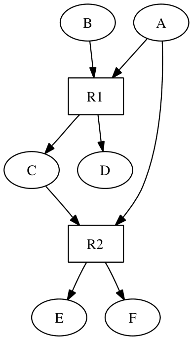
The metabolic network can be represented as a bipartite graph consisting of two types of nodes: metabolites and reactions. An example of a directed bipartite graph is shown in Fig. 1.1. In the directed bipartite metabolic graph, there is a link from a metabolite pointing to a reaction node if the metabolite is a reactant of the reaction, and a link from a reaction pointing to a metabolite node if the metabolite is a product of the reaction. In the bipartite metabolic graph, there are no direct links between two metabolites or two reactions. In chapter 2 of this thesis, we have studied the metabolic networks inside three organisms as a directed bipartite graph.
The metabolic networks are also sometimes represented as unipartite graphs (which could be directed or undirected) in which there is only one type of node (metabolite nodes or reaction nodes). In the undirected unipartite metabolite graph, for example, the nodes of the network represent metabolites, with edges between two metabolites if they participate in a single reaction. Similarly, in the undirected unipartite reaction graph, the nodes of the network represent reactions, with edges between two reactions if they share the same metabolite. In the directed unipartite reaction graph, there is a link pointing from one reaction node to another if the former produces a metabolite that is consumed by the latter.
The bipartite representation of the metabolic network has more information compared to the above unipartite representations. A more detailed description of the metabolic network would require three types of nodes: metabolites, reactions and enzymes. Such a tripartite network could additionally account for the correspondence between enzymes and reactions and regulatory interactions between metabolites and enzymes inside the cell.
1.2.2 Transcriptional regulatory network
Genes are segments of DNA that code for proteins inside the cell. Transcription is the process by which an enzyme, RNA polymerase, reads the sequence of bases on a gene and constructs an mRNA molecule from that sequence. Translation is the process in which a ribosome, a macromolecular assembly, reads the information contained in the mRNA molecule and synthesizes a protein molecule from the sequence on the mRNA molecule. Thus, each protein molecule is a product of the gene that codes for it. In turn, proteins are responsible for carrying out various functions inside the cell, including catalyzing reactions of the metabolic network as enzymes, building various cellular structures, etc.
The transcription of a gene to an mRNA molecule is also regulated by proteins. The proteins that regulate the expression of genes inside cells are referred to as transcription factors. A transcription factor may activate or inhibit the expression of a gene inside the cell by binding to regions upstream or downstream of the gene on the DNA molecule. This process may in turn facilitate or prevent RNA polymerase and rest of the transcription machinery from binding and initiating the transcription of the gene. Thus, the genes inside cells interact amongst each other via intermediate transcription factors to influence each other’s expression. This network of interacting genes inside the cell is referred to as the transcriptional regulatory network. This network may be represented by a graph in which every gene is represented by a node, and where an arrow from one gene node to another means that the former codes for a transcription factor that regulates the transcription of the latter gene.
A more detailed description of the transcriptional regulatory network would require us to characterize the regulatory links in the network as activating or repressing. Further, an input function needs to be specified for each gene node when more than one transcription factor regulates the expression of that gene in the network. In chapters 3 and 4 of this thesis, we have studied the part of the transcriptional regulatory network in E.coli that controls metabolism.
1.2.3 Other interaction networks
Inside the cell, the proteins interact with each other to influence each other’s activity. Extracellular signals are mediated to the inside of a cell by protein-protein interactions of signaling molecules. Proteins that interact for a long time with each other structurally can form part of a protein complex. A protein may also act as a carrier for another protein. A protein may interact briefly with another protein leading to a transfer of a phosphate group. These protein-protein interactions are crucial for living systems. We can represent various protein-protein interactions inside the cell by a network with nodes as proteins and links between two nodes representing a physical interaction between two proteins. Such networks are referred to as protein-protein interaction networks. The links between two nodes can be of various different types corresponding to different types of interactions between proteins.
1.2.4 Cell as a network of networks
It is important to emphasize that the metabolic, transcriptional regulatory and protein-protein interaction networks mentioned above are not independent of each other inside the cell. The state of the genes in the transcriptional regulatory network determines the activity of the metabolic network. The concentration of metabolites in the metabolic network determines the activity of transcription factors or proteins which regulate the expression of genes in the regulatory network. The protein-protein interactions determine the activity of various proteins inside the cell. Thus, the above mentioned and other biochemical networks together with the interactions at the interface of these networks form a ‘network of networks’ inside the cell that determines the overall behaviour of the organism.
1.3 Architectural features of large scale biological networks
Recent advances in the development of high-throughput data collection techniques coupled with the systematic analysis of fully sequenced genomes has generated detailed lists of molecular components inside various organisms. The available information has led to the mapping of different cellular networks inside many organisms. In this section, we review some of the known features of large scale metabolic and transcriptional regulatory networks. This also enables us to introduce more concretely the work done in this thesis.
1.3.1 Metabolic networks
The knowledge of enzymes along with their functional assignments have led to a reconstruction of nearly complete lists of organism specific metabolic reactions [22, 23, 24]. Jeong et al [25] studied the structure of the metabolic networks inside 43 different organisms. They represented the metabolic network as a bipartite graph with two types of nodes: metabolites and reactions. The degree of a node is defined as the number of links attached to that node in the graph [26, 27]. Since the metabolic network is a directed graph, each metabolite in the network has an in-degree and an out-degree. The in-degree of a node denotes the number of links that the node has to other nodes in the directed graph. The out-degree of a node denotes the number of links that start from the node to other nodes in the directed graph. The degree distribution of a graph, , gives the probability that a randomly selected node has exactly links in the graph [26, 27]. Jeong et al found both the in-degree and out-degree distribution of metabolites to approximate a power law form for the metabolic networks inside 43 organisms. is the degree exponent which they found to be universal and close to 2.2 for all the organisms studied, both for the in-degree and out-degree distribution.
Independently, Wagner and Fell [28] studied the large scale metabolic network of E. coli. They represented the E. coli metabolic network as two different unipartite graphs: metabolite graph and reaction graph [28]. Wagner and Fell also found the connectivity of the metabolites in the network to follow a power law distribution. The two independent studies by Jeong et al [25] and Wagner and Fell [28] show that most metabolites participate in a few reactions while there are a few metabolites which participate in many reactions in metabolite networks. The ubiquitous metabolites such as ATP that participate in several reactions and have a high degree are also referred to as hubs of the network.
The distance or shortest path between nodes and in a graph is defined as the minimum number of links that have to be traversed to reach from node to . The average path length of a graph is defined as the average over the shortest paths between all pairs of nodes in the network [26, 27]. The diameter of a graph is defined as the supremum of the shortest paths between all pairs of nodes in the network [26, 27]. The studies by Jeong et al [25] and Wagner and Fell [28] found the metabolic networks inside organisms to have the small-world [1] property, i.e., any two nodes in the system can be connected by relatively short paths along existing links. Jeong et al showed that the sequential removal of the high degree nodes or hubs from metabolic networks results in a sharp rise of network diameter as the network disintegrates into small isolated clusters. On the other hand, when they removed a set of randomly chosen metabolite nodes from the network, the average path length between the remaining nodes was not affected [25]. This observation led them to conclude that the hubs of the metabolic network are crucial for maintaining functionality of metabolic networks.
Ma and Zeng [29] have further explored the global connectivity structure of metabolic networks by classifying nodes in the metabolite graph into four subsets based on their mutual connectivity properties and location in the network: a giant strong component, in-component, out-component and an isolated subset. Two nodes and are said to strongly connected in a directed graph, if there is a path from to and from to in the graph. A strong component is a subset of nodes in the directed graph such that for any pair of nodes and in the subset there is a path from to and to in the directed graph. The largest strong component of a directed network is referred to as the giant strong component. The set of nodes that are not in the giant strong component but from which the nodes in the giant component can be reached forms the in-component. The set of nodes that are not in the giant strong component but that can be reached from the nodes in the giant component forms the out-component. The set of nodes that have no path to the nodes in the giant strong component forms the isolated subset. The decomposition of the metabolite nodes into the above mentioned four connected components revealed a ‘bow-tie’ macroscopic structure of the metabolic network [29]. The bow-tie structure of the metabolic network was similar to that observed by Broder et al for the World Wide Web [30]. In uncovering the bow-tie structure, Ma and Zeng removed the connections through the ubiquitous currency metabolites in the metabolic network. Csete and Doyle have argued that the bow tie architecture of the metabolic network with a conserved core and plug-and-play modularity around core can contribute toward robustness and evolvability of the system [31].
Ma and Zeng [29] also tried to account for the preferred directionality of reactions in the graph for the metabolic network, and found the average path length between metabolites to be almost double of that observed by Jeong et al. The average path length between nodes in the giant strong component was found to determine the average path length of the whole network. An alternative study by Arita [32] tried to account for the actual structural changes in connecting metabolites in the graph of the E. coli metabolic network, and found again the average path length to be almost double of that observed by Jeong et al. Thus, accounting for the directionality of reactions, activity of reactions and functional transfer of biochemical groups in a more biologically meaningful graph representation of the metabolic network gives an average path length larger than that obtained by Jeong et al.
The above mentioned studies of the structure of the metabolic networks have revealed a large variation in the metabolite connectivity inside these networks. It has been suggested that one of the important consequences of power law degree distribution is the vulnerability of the network to selective attack on hubs while being robust to random deletion of nodes from the network as most nodes are of low degree and their deletion does not change the average path length between remaining nodes in the network [33]. For the protein-protein interaction network of S. cerevisiae, it was shown that the essentiality of a protein is correlated with its degree in the network [34]. This observation has been suggested as evidence for the importance of the hubs in maintaining the overall structure and function of cellular networks. Although the role of high degree metabolites or hubs in maintaining the overall structure of the metabolic networks has been well emphasized in the literature, the role of low degree metabolites has attracted little or no attention.
In chapter 2 of this thesis, we show that certain low degree metabolites introduce fragility for flows in metabolic network. There we have used a computational method to determine essential reactions for growth in the metabolic networks inside three organisms. A reaction is designated as ‘essential’ if its knockout from the metabolic network renders the organism unviable. We show that the low degree metabolites as opposed to high degree metabolites explain essential reactions in metabolic networks [35]. It is the low degree metabolites that are critical from the point of view of functional robustness of the system.
In chapter 2, we also show that certain low degree metabolites lead to clusters of reactions with highly correlated reaction fluxes in the metabolic network. We then show that genes corresponding to reactions of such clusters predict regulatory modules in E. coli. Thus, the modularity observed by us at the metabolic level is also reflected at the genetic level. Our work therefore shows that low degree metabolites play a role in two hitherto unconnected properties of biological networks: on the one hand they cause certain reactions to become essential for the viability of the organism, and on the other hand they contribute to the modularity of biological networks.
1.3.2 Transcriptional regulatory networks
The available information regarding the target genes of transcription factors has led to a reconstruction of transcriptional regulatory networks inside model organisms like E. coli and S. cerevisiae [36, 37, 38, 39, 40]. The presently available transcriptional regulatory maps are highly incomplete due to ongoing annotation of the fully sequenced genomes. It has been estimated [41] that the coverage of the known transcriptional regulatory network of E. coli is only about of the actual network inside the organism.
The out-degree distribution for the known transcriptional regulatory network of E. coli and S. cerevisiae was shown to approximate a power law. However, the in-degree distribution for the two networks followed a restricted exponential function [37, 38]. This example shows that not all biological networks are characterized by a power law degree distribution of nodes. The out-degree of a node in the transcriptional regulatory network represents the number of target genes regulated by a transcription factor. The in-degree of a node in the transcriptional regulatory network represents the number of transcription factors regulating a target gene. The exponential in-degree distribution for the transcriptional regulatory network suggests that a very large promoter region required for the combinatorial regulation of a target gene by many transcription factors is highly unlikely inside the cell.
‘Network motifs’ have been defined as patterns of interconnections or subgraphs that are over-represented in a real network compared to randomized versions of the same network with similar local connectivity [37, 42]. Network motifs can be detected by algorithms that compare the patterns found in the real network to those found in suitably randomized networks. The method is analogous to detection of sequence motifs in genomes as recurring sequences that are very rare in random sequences. By studying the E. coli transcriptional regulatory network, Alon and colleagues found that the ‘feed-forward loop’ (FFL) is a motif in the regulatory network [37]. The structure of a feed-forward loop (FFL) motif is defined by a transcription factor X that regulates a second transcription factor Y, such that both X and Y jointly regulate a gene or operon Z. Other motifs found in the E. coli transcriptional regulatory network include the ‘single-input module’ (SIM) and ‘dense overlapping regulons’ (DOR) [37]. The structure of single-input module (SIM) is defined by a set of genes or operons that are controlled by a single transcription factor. The structure of dense overlapping regulons (DOR) is defined by a layer of overlapping interactions between genes or operons and a group of input transcription factors. Later, the motifs found in the E. coli transcriptional regulatory network were also found in the S. cerevisiae transcriptional regulatory network [38, 42].
By studying the dynamics of various motifs found in the regulatory networks, it has been shown that these motifs may perform important information processing tasks. The coherent feed-forward loop motif has been shown to filter out noise or spurious signals in the network [37, 16]. The single-input module motif was shown to help generate temporal programs of gene expression [37, 43]. Recent studies have shown that the appearance of same motifs in regulatory networks of E. coli and S. cerevisiae does not necessarily imply that these motifs are evolutionarily conserved [44, 45]. Evolution seems to have converged on the same patterns of interconnections in different organisms after a lot of tinkering perhaps due to the specific information processing tasks these motifs perform inside a cell [9, 45]. An objective of the exercise of detecting motifs in different biological networks is to create a library of motifs and their possible functions.
Ma et al [46] tried to decompose the E. coli transcriptional regulatory network into various connected components. They found that there were no strong components in the E. coli transcriptional regulatory network. This was consistent with earlier observations by Shen-Orr et al [37] that the network had no cycles of length 2. There were only autoregulatory loops in the presently known transcriptional regulatory network of E. coli [37]. Ma et al [46] found the structure of the E. coli transcriptional regulatory network to be hierarchical. A similar lack of strong components or cycles was also observed for the transcriptional regulatory network of S. cerevisiae [39]. The transcriptional regulatory network of E. coli had a five layered hierarchical architecture with genes at the top layer having no incoming links. Balaszi et al found that the genes at the top layer are regulated by distinct environmental signals in the transcriptional regulatory network of E. coli [47].
In chapters 3 and 4 of this thesis, we have studied the large scale structure and system level dynamics of the transcriptional regulatory network controlling metabolism in E. coli. Our study reinforces the hierarchical, essentially acyclic structure with environmental control of the genes belonging to the top layer of the regulatory network of E. coli, also found by previous studies mentioned above. Further, our dynamical study of regulatory network of E. coli metabolism elucidates the functional consequences of this observed architecture of the network [48]. We show that the regulatory network of E. coli metabolism exhibits two types of robustness. One, the regulatory network of E. coli metabolism exhibits an insensitivity to perturbations of gene configurations for a fixed environment, i.e., the system returns to the same attractor when gene configurations are perturbed for a fixed environment. Two, the regulatory network of E. coli metabolism exhibits a flexible response to changed environments, i.e., the system moves to a new attractor that enables it to maintain its key functionality when it encounters a changed environment in a sustained manner. The hierarchical acyclic architecture of the regulatory network of E. coli metabolism with control variables as external metabolites explains the observed robust dynamics of the system. Further, we observe a highly disconnected and modular architecture at the intermediate level of the hierarchical graph of the regulatory network. We find that the modules at the intermediate level of this hierarchical graph are regulated by different sets of environmental signals, and the modules interact only at the lowest level of the graph contributing to the robust response of the system to changed environments. This modular architecture of the regulatory network may also contribute towards the evolvability of the system. Thus, our study sheds new light on how structural design features of the regulatory network of E. coli contribute towards robustness and modularity of the system.
1.4 Methods for studying system level dynamics of large scale biological networks
Our work mentioned in the previous section employs graph theoretic and statistical methods to describe the structure of large scale metabolic and genetic regulatory network (like the other works reviewed in that section), but it also goes beyond structure to investigate flows and other dynamical phenomena. In this section, we mention some dynamical methods used for studying biological networks and discuss the kind of methods that are appropriate for a systems level study.
Many differential equations based models have been proposed and studied extensively to understand the dynamics of subsystems or pathways inside organisms. Two of the best examples are the E. coli chemotactic pathway and the segment polarity network of Drosophila melanogaster. Barkai and Leibler have studied extensively a kinetic model for the E. coli chemotactic pathway. They showed that the property of chemotactic adaptation (whereby a cell resets its tumbling frequency to the same basal value after a change of chemoattractant concentration) is robust to variations in a specific set of kinetic parameters. In their model, the robust behaviour of the system was a consequence of negative feedback, and this was later confirmed experimentally [49]. Yi et al showed that the robust behaviour of the E. coli chemotactic pathway is a consequence of a specific type of negative feedback control strategy, namely, integral feedback control [50] which is a commonly used strategy in engineering. von Dassow et al modelled the segment polarity network of Drosophila melanogaster using differential equations and showed that the spatial distribution of gene expression patterns was robust to changes in a set of initial conditions, rate constants or genetic perturbations [20]. They showed that positive feedback contributes to robustness in the model for the segment polarity network by amplifying the stimuli and enhancing the sensitivity of the system. Since then Ingolia has analyzed the model by von Dassow et al and showed that the bistability caused by positive feedback loops is responsible for the robust patten formation [51].
The above mentioned examples of differential equations based models for subsystems inside cells containing a few nodes have provided important insights about the robust behaviour of these subsystems. However, we expect to gain qualitatively different insights regarding the dynamical behaviour at the whole cell level by studying the dynamics of large scale biological networks that incorporate the collective functioning of a substantial fraction of the nodes in the system, compared to those obtained by studying the dynamics of smaller subsystems. At present, there is limited knowledge of kinetic parameters such as rate constants, enzyme concentrations, etc., for large scale biological networks. Further, the measured kinetic parameters for a given cell may show wide variation across the population of cells.
Due to paucity of kinetic data, a differential equation based simulation of large scale biological networks is not feasible at present and the large number of unknown parameters would also render the results of such a simulation difficult to interpret [52]. While deciding on a modelling approach to a large scale biological system, we need to account for the available knowledge about the system being studied. The choice of the method and the level of abstraction would also depend upon the questions we wish to address for the biological system at hand. In the absence of large scale kinetic data, alternative modelling approaches such as flux balance analysis (FBA) and Boolean networks can be used to simulate the dynamics of metabolic networks and genetic regulatory networks, respectively.
At present, the list of reactions along with the stoichiometric coefficients of the involved metabolites is largely known for metabolic networks inside many single celled organisms. However, we currently lack the knowledge of kinetic rate constants for most reactions that can occur inside the cell. Due to lack of kinetic data, constraint based modelling approaches such as flux balance analysis (FBA) [53, 54, 55, 11] can be used to perform a steady state analysis of the large scale metabolic networks. FBA is a computational technique that can be used to determine the steady state fluxes of all reactions in the metabolic network and predict the growth rate of the cell for a given nutrient medium. The key requirement for FBA technique is the knowledge of network structure along with stoichiometric coefficients of the involved metabolites which is largely known for many organisms. The predictions of FBA for few reaction fluxes and growth rate of E. coli under few minimal media have been shown to have good agreement with experimentally measured values [55, 56]. In chapter 2 of this thesis, we have used FBA to determine essential reactions for growth in the metabolic networks for E. coli, S. cerevisiae and S. aureus.
In the case of genetic regulatory networks, the current availability of biological data is limited to network structure and the information regarding the nature of regulatory links, i.e., activating or repressing. When more than one regulatory link converges at a single gene in the network, an input function needs to be specified for the gene. In the absence of quantitative data on genetic regulatory networks, the Boolean network approach may be used to perform qualitative simulations. Kauffman proposed the framework of Boolean networks to study the dynamics of genetic regulatory networks [57, 58, 59]. The Boolean approach provides a coarse grained description of the dynamics of genetic regulatory networks where each gene in the network is in one of the two states: active or inactive. In this approach, the state of each gene at a given time instant is determined by the state of its input genes at the previous time instant based on a Boolean input function. The input function may be written in terms of the AND, OR and NOT Boolean operators. This is a discrete dynamical system; the genes’ states may be updated synchronously or asynchronously. Boolean network models of small cellular subsystems have also provided useful biological insights [60, 61, 62, 63, 64]. Recently, two databases for large scale transcriptional regulatory networks inside model organisms, E. coli and S. cerevisiae, have been reconstructed using empirical data that contain both the network structure and Boolean input functions [41, 65]. In chapter 3 of this thesis, we have used the Boolean approach to study the dynamics of the large scale genetic network controlling E. coli metabolism as represented in the database iMC1010v1 [41].
1.5 Thesis organization
The subsequent chapters in this thesis are organized as follows:
-
•
Chapter 2 studies the structure and dynamics of the metabolic networks inside three organisms. We determine metabolites based on their low degree of connectivity in the metabolic network. We show that certain low degree metabolites lead to clusters of highly correlated reactions in the metabolic network. We find that these clusters at the metabolic level correspond to regulatory modules at the genetic level. The computational technique of flux balance analysis (FBA) is then used to determine ‘essential’ reactions for growth in the metabolic networks of E. coli, S. cerevisiae and S. aureus. We show that most essential reactions in metabolic networks are explained by their association with a low degree metabolite. In this chapter, we show that low degree metabolites are implicated in two seemingly unrelated properties in metabolic networks: modularity and essentiality.
-
•
Chapter 3 studies in detail the dynamics of the large scale genetic network controlling E. coli metabolism. Using the information contained in a previously published database [41] representing the genetic network controlling E. coli metabolism, we construct an effective Boolean dynamical system of genes and external metabolites describing the network. We study the dependence of the attractors of this Boolean dynamical system on the initial conditions of genes and state of the external environments. We find that the attractors of the Boolean dynamical system are fixed points or low period cycles for any fixed environment. We show that the system exhibits the property of homeostasis in that the attractor is highly insensitive to initial conditions or perturbation of genes for a fixed environment. However, we find that the attractors corresponding to different environments have a wide variation. We also show that for most environmental conditions, the attractors of the genetic network allow close to optimal metabolic growth. In this chapter, we show that the genetic network controlling E. coli metabolism simultaneously exhibits the twin dynamical properties of homeostasis and flexibility of response.
-
•
Chapter 4 studies the design features of the genetic network controlling E. coli metabolism in order to understand the origin of observed dynamical properties of homeostasis and response flexibility. We find that the genetic network controlling E. coli metabolism is an essentially acyclic graph. The root nodes of this acyclic graph are external metabolites that act as control variables of the dynamical system. The leaf nodes of the acyclic graph are the genes coding for enzymes while the genes coding for transcription factors are at the intermediate level. We shown that deleting the leaf nodes corresponding to the enzyme coding genes along with their links from the full graph leads to a subgraph with many disconnected components that may be regarded as modules of the genetic network. The localization and dynamical autonomy of the disconnected components or modules may contribute towards evolvability of the network. In this chapter, it is shown that the architecture of the genetic network endows the system with the twin properties of homeostasis and flexibility of response.
-
•
Chapter 5 is a perspective of the work reported in this thesis in relation to the overall subject. It discusses some of the limitations associated with this work. It also suggests some future directions of research based on work reported here.
-
•
Appendix A lists the 85 UP-UC clusters in the E. coli metabolic network.
-
•
Appendix B reviews the computational technique of flux balance analysis (FBA).
-
•
Appendix C describes various computer programs used to obtain results reported in this thesis. These programs can be downloaded from the associated website: http://areejit.samal.googlepages.com/programs.
Chapter 2 Low degree metabolites enhance modularity and explain essential reactions in metabolic networks
In this chapter, we have studied the metabolic networks of Escherichia coli, Saccharomyces cerevisiae and Staphylococcus aureus. We first locate metabolites based purely on their low degree in the metabolic network. We then show that certain low degree metabolites contribute to a rigidity or coherence of reaction fluxes in the metabolic network resulting in clusters of highly correlated reactions. We find that these clusters of metabolic reactions in the E. coli metabolic network predict genetic regulatory modules, as captured in the structure of operons, with a high probability. We then use a computational method to determine the essential reactions for growth in the metabolic networks of E. coli, S. cerevisiae and S. aureus. We show that most essential metabolic reactions in E. coli, S. cerevisiae and S. aureus can be explained by the fact that they are associated with a low degree metabolite.
2.1 ‘Uniquely Produced’ (‘Uniquely Consumed’) metabolites and their associated reactions
It is convenient to represent the metabolic network as a bipartite graph consisting of two types of nodes: metabolites and reactions. In a directed bipartite graph, there are two types of links: (a) from metabolite nodes to reaction nodes and (b) from reaction nodes to metabolite nodes. The first type of links defines the reactants. The second type of links defines the products. In a bipartite graph, there are no links between two similar types of nodes.
We have designated a metabolite as ‘uniquely produced’ or ‘UP’ (‘uniquely consumed’ or ‘UC’), if there is only a single reaction in the metabolic network that produces (consumes) the metabolite [35]. A UP(UC) metabolite has in-degree (out-degree) equal to unity in the bipartite graph. A metabolite that is both UP and UC may be designated as a ‘UP-UC metabolite’ [35]. A UP-UC metabolite has both in-degree and out-degree equal to unity. Such a metabolite has degree two in the network. In general, a metabolite that is either UP or UC or both has a low degree in the metabolic network as it participates in very few reactions.
We have designated a reaction as ‘uniquely producing’ or ‘UP’ (‘uniquely consuming’ or ‘UC’), if it produced (consumed) a UP(UC) metabolite in the bipartite metabolic network [35]. A reaction is UP(UC), if it is the only process by which some metabolite can be produced (consumed) in the complete metabolic network. We designate reactions in the metabolic network that are either UP or UC or both as ‘UP/UC reactions’.
The metabolic network is an input-output network which takes in nutrients from the external environment as inputs and produces key molecules contributing towards growth and maintenance of the cell as outputs. In this chapter, we have studied the metabolic networks inside three organisms: E. coli (version iJR904 [66]), S. cerevisiae (version iND750 [67]) and S. aureus (version iSB619 [68]). The databases iJR904, iND750 and iSB619 for E. coli, S. cerevisiae and S. aureus, respectively, have been reconstructed using the annotation of fully sequenced genomes for these organisms and biochemical literature sources. The databases were downloaded from the website [22]. The reactions inside these metabolic network databases can be broadly classified into internal and transport reactions. The transport reactions in the metabolic network represent transport processes of metabolites across the cell boundary. The internal reactions in the metabolic network are confined to the cell boundary. In addition to internal and transport reactions, the metabolic network databases considered here contain a fictitious reaction referred to as the biomass reaction representing the ratios of various metabolic precursors that are required for unit biomass production or growth of the organism.
For convenience, the metabolites that can be transported across the cell boundary are represented by two nodes in the metabolic network databases considered here. One of the nodes represents the external version of the metabolite and the other node represents the internal version of the metabolite, and the transport of the metabolite across the cell boundary is treated as a dynamical reaction in the above mentioned databases converting one type of node into another. In the databases considered here, most external metabolites are usually involved in only two unidirectional transport reactions in the metabolic network representing their transport process across the cell boundary. One of the two reactions transports a external metabolite into the cell while the other transports it outside the cell. Thus, most external metabolites in these metabolic network databases satisfy the property of UP or UC or both. We do not consider the external metabolites while determining the set of UP(UC) metabolites in the network as the external metabolite nodes are a matter of convention in the databases. We consider only the internal metabolites while determining the set of UP(UC) metabolites in the network.
2.1.1 Detection of UP(UC) metabolites and reactions
The list of reactions in a reconstructed metabolic network for an organism includes both reversible and irreversible reactions. Starting from the reconstructed metabolic network of an organism, we prepare a list of metabolic reactions that has each reversible reaction in the original network replaced by two unidirectional reactions (one reaction each for the forward and the backward direction). From this list of unidirectional metabolic reactions, construct a matrix = of dimensions , where is the number of internal metabolites and is the number of reactions in the network. The rows of matrix correspond to metabolites and the columns correspond to reactions in the metabolic network. The matrix element is set equal to -1, if metabolite is consumed in reaction , +1 if metabolite is produced in reaction , and 0 if metabolite does not participate in reaction . The matrix is a compact representation of the bipartite metabolic graph.
A UP(UC) metabolite has in-degree (out-degree) equal to unity in the bipartite metabolic graph. A metabolite in the network is UP(UC), if the row of matrix has exactly one entry that equals -1 (+1). A UP-UC metabolite has in-degree and out-degree equal to unity in the bipartite metabolic graph. A metabolite in the network is UP-UC, if the row of matrix has exactly one entry that equals -1, one entry that equals +1 and has all other entries 0. A reaction is UP(UC), if the column of matrix has at least one entry +1 (-1) such that the row corresponding to the entry +1 (-1) in column has no other entry equal to +1 (-1).
As mentioned earlier, we do not consider the external metabolites while determining the set of UP(UC) metabolites. This amounts to excluding the rows corresponding to external metabolites from the matrix for the computation of UP(UC) metabolites. Thus, the matrix does not contain any rows corresponding to external metabolites and the rows of matrix correspond only to internal metabolites in the network. The biomass reaction which defines the ratios of various metabolic precursors that are required for the unit biomass production of the organism is also included in the list of reactions while determining the UP(UC) metabolites. Usually, the last column of the bipartite matrix corresponds to the biomass reaction.
2.1.2 UP(UC) statistics for the metabolic networks of E. coli, S. cerevisiae and S. aureus
The databases were downloaded from the website [22]. The E. coli metabolic network iJR904 accounts for 761 metabolites participating in 931 reactions (686 irreversible and 245 reversible reactions). The S. cerevisiae metabolic network iND750 accounts for 1061 metabolites participating in 1149 reactions (719 irreversible and 430 reversible reactions). The S. aureus metabolic network iSB619 accounts for 645 metabolites participating in 644 reactions (423 irreversible and 221 reversible reactions).. Following the steps outlined in section 2.1.1, the bipartite matrix was constructed for the three metabolic networks. We found the dimensions (,) of matrix to be (618,1177), (945,1580) and (561,866) for the metabolic networks of E. coli, S. cerevisiae and S. aureus, respectively. In obtaining the bipartite matrix for the three metabolic networks, each reversible reaction was converted into two one sided reactions. Further, the biomass reaction was added to the list of metabolic reactions. The number of external metabolites in the metabolic networks of E. coli, S. cerevisiae and S. aureus was 143, 116 and 84, respectively. The rows corresponding to these external metabolites were not included in the matrix for determining UP or UC metabolites.
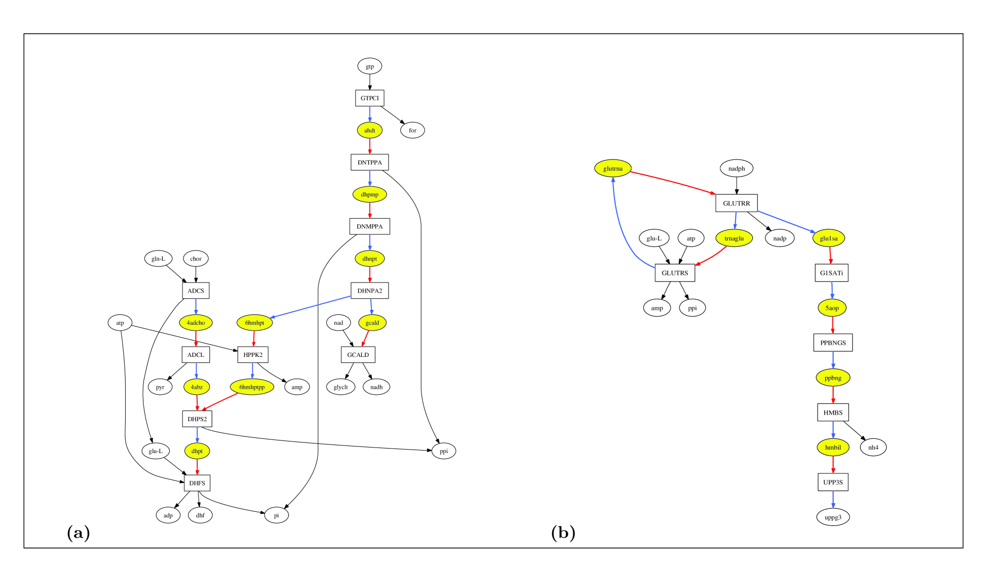
Using the bipartite matrix for each one of the three organisms, we determined UP(UC) metabolites and reactions in the metabolic networks of E. coli, S. cerevisiae and S. aureus. We found the number of UP(UC) metabolites in the metabolic networks of E. coli, S. cerevisiae and S. aureus to be 291 (285), 395 (376) and 282 (237), respectively. We found the number of UP-UC metabolites in the metabolic networks of E. coli, S. cerevisiae and S. aureus to be 185, 178 and 145, respectively. Examples of UP-UC metabolites in E. coli and S. aureus networks are shown in Fig. 2.1. We found the number of UP(UC) reactions in the metabolic networks of E. coli, S. cerevisiae and S. aureus to be 289 (272), 391 (370) and 277 (218), respectively. The number of reactions that were either UP or UC or both (the ‘UP/UC reactions’) in the metabolic networks of E. coli, S. cerevisiae and S. aureus were found to be 418, 583 and 376, respectively.
2.2 ‘UP-UC cluster’ of reactions
A UP-UC metabolite has one reaction that produces it and one reaction that consumes it in the metabolic network. A steady state is defined as one where all metabolite concentrations and reaction velocities are constant. In any steady state, the flux of the reaction producing a UP-UC metabolite is always proportional to the flux of the reaction consuming the metabolite, with the proportionality constant determined by the stoichiometric coefficients of the metabolite in the two reactions. Then, maintaining the steady state requires the enzymes of the two reactions associated with a UP-UC metabolite to be simultaneously active. This raises the question as to whether the genes coding for enzymes of the two reactions associated with a UP-UC metabolite are coexpressed. We have defined a ‘UP-UC cluster’ of reactions as a set of reactions connected by UP-UC metabolites [35]. Examples of UP-UC clusters of reactions in the metabolic networks of E. coli and S. aureus are shown in Fig. 2.1. In steady state, fluxes of all reactions that are part of a single UP-UC cluster are proportional to each other. Fixing the flux of any reaction in a UP-UC cluster fixes the fluxes of all other reactions in the cluster under steady state. Further, for any steady state analysis, each UP-UC cluster can be replaced by a single effective reaction and this can be used to coarse-grain metabolic networks [70, 71]. Notice that UP-UC clusters include linear pathways but can lead to branched or cyclic structures as shown in Fig. 2.1. UP-UC clusters of reactions are special cases of reaction/enzyme subsets [70, 71, 72], co-sets [73, 74] and fully coupled reactions [75] that have been discussed earlier in the literature.
2.2.1 Algorithm to determine UP-UC clusters
We now describe in detail the algorithm to determine UP-UC clusters in any metabolic network.
-
1.
Starting from the reconstructed metabolic network of an organism, construct the bipartite matrix of dimensions , where is the number of internal metabolites and is the number of reactions in the network as described in section 2.1.1.
-
2.
In the matrix , determine the rows corresponding to UP-UC metabolites as described in section 2.1.1.
-
3.
Obtain a matrix from matrix by setting every entry of each row in that corresponds to a non UP-UC metabolite equal to zero, i.e., delete all links in the graph except those going into or out of UP-UC metabolites.
-
4.
From the matrix , construct a reaction-reaction graph in which each node corresponds to a reaction. The adjacency matrix = of this graph is defined as = 1 if = 1 and = -1, else = 0. The matrix represents a directed graph.
-
5.
The weak components of size 2 of the graph are the various UP-UC clusters. These are obtained as follows: First convert the directed graph into the associated undirected graph by dropping all the directions of the arrows, i.e., = 1 if = 1 or = 1 or both, else = 0. Two nodes and in are said to be weakly connected if there exists a path between them in the associated undirected graph . A weak component is a maximal set of nodes that are weakly connected to each other.
By construction, if two reaction nodes and are adjacent (i.e., connected by a link) in , there exists a UP-UC metabolite that is produced in one of those reactions and consumed in the other. Thus, the fluxes of those two reactions will have a constant ratio in all steady states. This logic extends to entire connected cluster in to which those reactions belong.
Note that a choice has to be made as to whether to include or exclude the biomass reaction from the list of reactions in matrix and . Its inclusion/exclusion gives slightly different results for the set of UP-UC metabolites and their clusters. The biomass reaction should be included in the matrix in steps 1-2 above (identification of UP-UC metabolites), for if it is not, then those biomass metabolites which are consumed by only one reaction other than the biomass reaction get identified as UC metabolites resulting in some spurious UP-UC clusters. However, in the matrix (steps 3-5) it is a matter of convention whether the biomass reaction is included or not; results in the two cases are different but each is valid in its own right. The results reported in this chapter correspond to the following choice: In steps 1-2 above, the matrix includes the biomass reaction and in steps 3-5 the matrix excludes it. When the biomass reaction is included in the matrix the size of the largest UP-UC cluster increases. A program to determine UP-UC clusters in the E. coli metabolic network is contained in Appendix C.
2.3 UP-UC clusters predict regulatory modules in E. coli
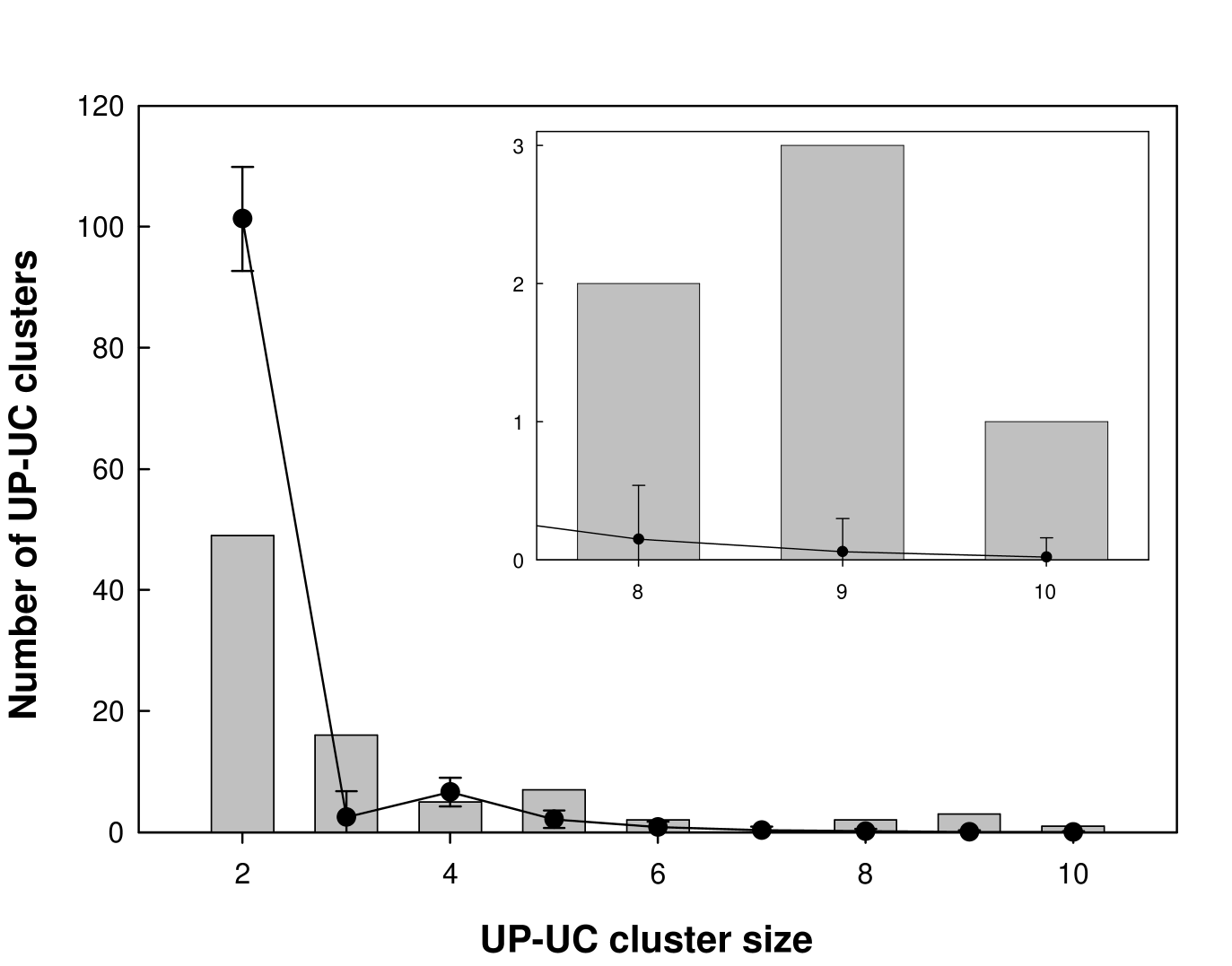
We used the algorithm mentioned in section 2.2.1 to determine UP-UC clusters in the E. coli metabolic network iJR904. The total number of UP-UC clusters in the E. coli metabolic network was found to be 85. The list of 85 UP-UC clusters in the E. coli metabolic network is contained in Appendix A. The size distribution of UP-UC clusters in the E. coli metabolic network is shown by grey bars in Fig. 2.2 and listed in Table 2.1.
Since the fluxes of reactions forming a UP-UC cluster have fixed ratios with respect to each other for all steady states, the set of genes that code for enzymes catalyzing various reactions of the cluster may be expected to be coregulated forming a transcriptional module. The bacteria E. coli is a prokaryote. In prokaryotes, the genes are grouped into transcriptional modules called operons. An operon is a set of genes which are transcribed into a single mRNA molecule that may code for more than one protein. The set of genes that form a single operon are therefore guaranteed to be coexpressed. We investigated whether the genes coding for enzymes catalyzing reactions of a UP-UC cluster are part of the same operon in E. coli. At present, the genes corresponding to enzymes of reactions that constitute the E. coli metabolic network iJR904 have been identified for only part of the network. Of the 85 UP-UC clusters in E. coli, only 69 UP-UC clusters had two or more reactions with known corresponding genes. The regulation of these 69 UP-UC clusters was investigated using the known operon information from RegulonDB [36] and Ecocyc [24] databases for E. coli. Genes of reactions within 85 UP-UC clusters for E. coli that belong to the same operon are indicated in the table listed in Appendix A. For 42 of the 69 UP-UC clusters, two or more genes of the cluster were found to be part of the same operon. Furthermore, we found that 36 of these 42 UP-UC clusters had at least half of their genes belonging to the same operon. For 21 UP-UC clusters, we found all reactions in a cluster to be covered by the same operon in the sense that at least one gene catalyzing each reaction in the set belonged to the same operon.
The following test was performed to show that two genes belonging to a UP-UC cluster in E. coli have greater probability of lying on the same operon than otherwise expected. We found that there were 251 unique genes catalyzing various reactions in the 69 UP-UC clusters. If we randomly pick any two of these 251 genes, the probability that the two genes lie on the same operon is 0.0057. If we randomly pick a pair of genes that belong to the same UP-UC cluster from this set of 251 genes, the probability that the two genes lie on the same operon is 0.29. Thus, genes belonging to a UP-UC cluster have a much greater probability of being coregulated than otherwise. This shows that the set of genes that correspond to a UP-UC cluster in the E. coli metabolic network are strongly correlated with regulatory modules at the genetic level. Our analysis here rests only on the available operon data for E. coli. However, it is possible that two genes which do not belong to the same operon are coexpressed inside the cell. For example, a set of genes that are regulated by the same transcription factor inside the cell may be coexpressed. So, it is possible that UP-UC clusters may find even greater correspondence with regulatory modules when expression data for E. coli is analyzed.
| Size of UP-UC | Number of clusters | Number of clusters in |
|---|---|---|
| cluster | in real network | randomized networks |
| Mean S.D. | ||
| 2 | 49 | 101.32 8.60 |
| 3 | 16 | 22.49 4.28 |
| 4 | 5 | 6.62 2.38 |
| 5 | 7 | 2.15 1.44 |
| 6 | 2 | 0.84 0.89 |
| 7 | 0 | 0.34 0.57 |
| 8 | 2 | 0.15 0.39 |
| 9 | 3 | 0.06 0.24 |
| 10 | 1 | 0.02 0.14 |
2.4 Large UP-UC clusters are over-represented in the real metabolic network
The bunching up of UP-UC metabolites next to each other in the metabolic network results in formation of UP-UC clusters with more than two reactions. We asked the question: Is it expected that a network like the E. coli metabolic network of 618 internal metabolites and 1177 reactions with 185 UP-UC metabolites will have a size distribution of UP-UC clusters as given in Table 2.1? To answer this question, we compared the distribution of UP-UC clusters in the real E. coli metabolic network with a suitably randomized version of the original network. The randomized network has the same number of metabolite nodes and reaction nodes and the same number of incoming and outgoing links at each node as the real E. coli metabolic network.
The randomized networks with same local connectivity as the real E. coli metabolic network were generated using the following algorithm. Starting from the reconstructed metabolic network for E. coli, generate the bipartite matrix following the steps outlined in section 2.1.1. Starting from the matrix for the real E. coli metabolic network, we generated randomized networks keeping the degree of each metabolite and reaction node unchanged [76, 77]. It is important to distinguish between two kinds of links. The entries +1 in the matrix represent the links coming into a metabolite node from a reaction node and the entries -1 in the matrix represent the links going out of a metabolite node to a reaction node. We divided all links or edges in the bipartite graph into these two groups. Two links are then randomly selected in one of these two groups and swapped. Before swapping, we ensure that the metabolite involved in any link is not already involved as a reactant or product in the reaction corresponding to the other link (otherwise, we could end up with metabolites being consumed and produced in the same reaction). Furthermore, links corresponding to the biomass reaction are not picked for swapping. This process of selecting a random pair of links was repeated 18000 times. It was verified that more than 99.9% of the links were visited at least once. Starting from the real metabolic network, this procedure was repeated 1000 times (with different random number seeds), to generate 1000 randomized networks.
We determined the UP-UC clusters for each of the 1000 realizations of the randomized network. The cluster size distribution averaged over 1000 realizations of the randomized network is shown by the black line in Fig. 2.2. From the Fig. 2.2, we can see that the actual metabolic network of E. coli has its UP-UC metabolites bunched up next to each other, forming larger clusters than may be expected in random networks with the same local connectivity properties as the original network. ‘Network motifs’ have been defined as patterns of interconnections that occur in different parts of a network at frequencies much higher than those found in randomized networks [37, 42, 9, 78]. Thus, larger size (size ) UP-UC clusters are over-represented in the real E. coli metabolic network, and may be collectively considered as analogous to a network motif. The smaller size () UP-UC clusters are under-represented in the real E. coli metabolic network, and may be collectively considered analogous to an ‘anti-motif’. We obtained qualitatively similar results for the metabolic networks of S. cerevisae and S. aureus. Thus, real metabolic networks contain many more large UP-UC clusters than are expected in the randomized networks with the same local connectivity. Larger UP-UC clusters in the real network may facilitate the regulation of certain metabolic pathways inside the organism.
2.5 Essential metabolic reactions
The metabolic network is extremely flexible to allow an organism to survive and grow under varied environmental conditions. Organisms in the course of evolution have developed redundancies in their intracellular machinery in order to tolerate random failures (e.g., random mutations, etc). Yet certain failures in the system may turn out to be lethal for the survival of the organism. For example, a mutation in a gene may result in its coded protein being nonfunctional. Enzymes are proteins that catalyze reactions in the metabolic network. If an enzymatic protein becomes nonfunctional due to mutation in its coding gene, it may tantamount to a loss in the capability of the cell to carry out certain reactions catalyzed by that enzyme. Such a loss of ability to carry out certain biochemical reactions in the cell may turn out to be lethal for the organism as the lost reactions may be essential for growth under certain environmental conditions. A reaction is designated as ‘essential’ for certain growth medium, if its knockout from the metabolic network results in the organism being unable to grow under that medium.
2.5.1 Determination of essential reactions
In practice, we cannot directly knockout a reaction in the metabolic network via molecular biology techniques in order to experimentally determine essential reactions for the survival of an organism. However, it is possible to knockout genes via molecular biology techniques and observe the effect of the knockout on the viability of the organism for different growth media in the wet lab. The knockout of a gene in effect results in the coded protein or enzyme being eliminated from the network. This would in effect result in the elimination of one or more reactions from the metabolic network that are catalyzed by the enzyme. If the knockout of a gene renders the organism unviable for certain growth medium then the gene is deemed ‘essential’ for that growth medium. The overall process of determining essential genes using in vivo experiments is very tedious and time consuming. Also, there is not always a one to one correspondence between genes and reactions in the network, and it may be difficult to determine essentiality of certain reactions using wet lab experiments. This is because the knockout of a single gene may in turn eliminate an enzyme that may catalyze multiple reactions in the metabolic network which are all removed from the network as a result of the knockout of the gene.
We have used a here computational method to determine essential reactions in metabolic networks. This method relies on the technique of flux balance analysis (FBA) [79, 80, 81, 82, 83, 84, 53, 85, 86, 87, 54, 55, 56, 88, 89, 66, 90, 91, 67, 92, 11]. Flux balance analysis (FBA) is a computational modelling technique which can be used to obtain the maximal growth rate of the organism supported by the metabolic network for any given nutrient medium. It also gives the steady state fluxes of all reactions in the metabolic network for any medium (for a detailed description of FBA see Appendix B). We have used FBA to study the metabolic networks of E. coli (version iJR904), S. cerevisiae (version iND750) and S. aureus (version iSB619).
FBA technique was used to compute fluxes of all metabolic reactions and optimal growth rate of E. coli for all possible aerobic minimal media. Any aerobic minimal media is characterized by availability of a single carbon source and key inorganic sources (ammonium, Fe2+, oxygen, phosphate, potassium, proton, sodium, sulfate and water) for the uptake of E. coli. If for a particular medium, the optimal growth rate obtained using the technique of FBA is zero, then under that condition the metabolic network does not permit the organism to grow. Using FBA, it was found that the E. coli metabolic network iJR904 supports nonzero growth under 89 aerobic minimal media [93]. Further, a reaction in the E. coli metabolic network was designated as ‘active’ if it has a nonzero flux value for at least one of the 89 minimal media, and ‘inactive’ otherwise. Similarly, using FBA, it was found that the metabolic networks for S. cerevisiae and S. aureus supported nonzero growth under 43 and 27 aerobic minimal media respectively. These 89, 43 and 27 aerobic minimal media that supported growth in E. coli, S. cerevisiae and S. aureus, respectively, were designated as ‘feasible minimal media’.
We used FBA to computationally determine essential reactions in the metabolic networks of E. coli, S. cerevisiae and S. aureus. We checked the effect of ‘switching off’ or removal of a reaction one by one from the metabolic network on the optimal growth rate of the organism obtained using FBA for different feasible minimal media. In FBA, a reaction can be switched off or removed from the network by setting the maximum flux (a parameter input in FBA) through the reaction equal to zero. We designated a reaction as ‘essential’ for a particular minimal medium, if switching the reaction off resulted in a zero optimal growth rate for that medium. We designated a reaction as ‘globally essential’ for an organism, if it was essential for all its feasible minimal media under aerobic conditions. A program to determine essential reactions in the E. coli metabolic network iJR904 is contained in Appendix C.
The number of essential reactions for each of the 89 minimal media varied between 200 and 240 and the number of globally essential reactions was 164 for the E. coli metabolic network. The number of essential reactions for each of the 43 minimal media varied between 165 and 187 reactions and the number of globally essential reactions was 127 for the S. cerevisiae metabolic network. The number of essential reactions for each of the 27 minimal media varied between 222 and 256 reactions and the number of globally essential reactions was 196 for the S. aureus metabolic network.
2.6 Essential metabolic reactions are largely explained by UP/UC structure
2.6.1 Most globally essential reactions can be tagged by a UP or UC metabolite
We found a set of 164 metabolic reactions to be globally essential in the E. coli metabolic network. Similarly, the number of globally essential reactions in S. cerevisiae (S. aureus) metabolic network was found to be 127 (196). We then tried to understand why certain reactions happen to be globally essential in terms of the underlying structure of the metabolic network. Notice that if a UP or UC metabolite is an essential intermediate in the production of a metabolite that are part of the biomass reaction then that reaction responsible for the production or consumption of that UP or UC metabolite becomes essential for the growth of the organism. Of the 164 globally essential reactions in the E. coli metabolic network, 133 were found to be either UP or UC. Similarly, a high fraction of globally essential reactions in the metabolic networks of S. cerevisiae and S. aureus were found to be UP or UC (see Table 2.2). This explains why the subset of 133, 86 and 157 reactions are globally essential in E. coli, S. cerevisiae and S. aureus, respectively, namely, there is simply no other path around these reactions in the entire network to produce or consume some metabolite that is presumably required for the eventual production of biomass.
The probability of such a high overlap between the set of globally essential reactions and set of UP/UC reactions occurring by pure chance is very small. To quantify this, the result was compared to a null model in which the two sets corresponding to globally essential reactions and UP/UC reactions were considered to be independent of each other. The total number of reactions in the E. coli metabolic network is 1176. The number of globally essential reactions is 164 and the number of UP/UC reactions is 417 for the E. coli network. The probability that out of a set of 1176 reactions in E. coli, two independently chosen subsets of size 417 and 164 will have an intersection of 133 or greater is (any one or both of the subsets is chosen randomly). Similarly, we obtained very small values for the metabolic networks of S. cerevisiae and S. aureus (see Table 2.2).
In an earlier paper [94] Mahadevan and Palsson had determined the ‘lethality fraction’ for each metabolite in the network. The lethality fraction of a metabolite was defined as the fraction of reactions in which the metabolite is involved that are essential. Mahadevan and Palsson had observed that this lethality fraction of the low degree metabolites is on average comparable to high degree metabolites. In particular, they found that some metabolites with in-degree and out-degree unity (that we have designated as UP-UC metabolites) have lethality fraction unity. We have presented here a stronger result regarding the role of low degree metabolites: most globally essential reactions involve at least one UP or UC metabolite. The essential reactions may involve other metabolites of higher degree, but their essentiality is due to their uniqueness in producing or consuming a UP or UC metabolite.
| Organism | E. coli | S. cerevisiae | S. aureus |
| Total number of reactions | 1176 | 1579 | 865 |
| Number of globally essential reactions | 164 | 127 | 196 |
| Number of globally essential reactions | 133 | 86 | 157 |
| that are UP or UC in the entire network | () | () | () |
| Number of globally essential reactions | 156 | 117 | 182 |
| that are UP or UC in the reduced network | () | () | () |
| Organism | E. coli | S. cerevisiae | S. aureus |
|---|---|---|---|
| Number of reactions in the | 1176 | 1579 | 865 |
| original network | |||
| Number of UP reactions in the | 289 | 391 | 277 |
| original network | |||
| Number of UC reactions in the | 272 | 370 | 218 |
| original network | |||
| Number of UP/UC reactions in the | 417 | 583 | 376 |
| original network | |||
| Number of blocked reactions | 290 | 800 | 294 |
| Number of UP/UC reactions in the | 136 | 386 | 174 |
| original network that are blocked | |||
| Number of reactions in the | 886 | 779 | 571 |
| reduced network | |||
| Number of UP reactions in the | 245 | 218 | 224 |
| reduced network | |||
| Number of UC reactions in the | 245 | 218 | 181 |
| reduced network | |||
| Number of UP/UC reactions in the | 352 | 306 | 276 |
| reduced network | |||
| Number of UP/UC reactions in the | 71 | 109 | 74 |
| reduced network that are not | |||
| UP/UC in the original network |
2.6.2 Almost all globally essential reactions are UP/UC in the ‘reduced network’
It was shown above that 133 out of 164 globally essential reactions were associated with a UP or UC metabolite in the E. coli metabolic network. To understand the remaining globally essential reactions, a reduced or pruned version of the E. coli network was considered.
The databases of reconstructed metabolic networks that have been used here contain certain reactions that can only have a zero flux value under any steady state due to stoichiometric reasons. Such reactions have been referred to as ‘strictly detailed balanced’ reactions [95, 96] or ‘blocked’ reactions [75] (see section B.2 in Appendix B for more details). The blocked reactions can be removed from the reconstructed metabolic networks for any steady state analysis. We used a previously described algorithm by Burgard et al [75] to determine the blocked reactions in the metabolic networks of E. coli, S. cerevisiae and S. aureus. This algorithm to determine blocked reactions has been described in detail in section B.2.1 in Appendix B. A program to determine blocked reactions in the E. coli metabolic network is contained in Appendix C. The number of blocked reactions in the metabolic networks of E. coli, S. cerevisiae and S. aureus were found to be 290, 800 and 294, respectively (for details see Table 2.3). We removed the 290 blocked reactions in the E. coli metabolic network from the list of 1176 reactions to obtain the ‘reduced network’ of 886 reactions in E. coli. We emphasize that the removal of blocked reactions from the original network does not affect our results obtained using FBA for any of the 89 minimal media considered for E. coli. The 290 blocked reactions removed from the original E. coli metabolic network of 1176 reactions had a zero flux value for all 89 minimal media studied here. Further, since the blocked reactions are guaranteed to have a zero flux value for any minimal media, they can be never essential. So, the set of essential reactions obtained by implementing FBA on the reduced network is exactly the same as that obtained from the original network for any minimal media. Thus, the set of 164 globally essential reactions is the same for the original network of 1176 reactions and the reduced network of 886 reactions in E. coli. Similarly, the reduced networks for S. cerevisiae and S. aureus were obtained by removing the corresponding blocked reactions from the original network (see Table 2.3).
The set of UP(UC) metabolites was then determined for the reduced metabolic network obtained after removing blocked reactions from the original network. A metabolite that was not UP(UC) in the original metabolic network can become UP(UC) in the reduced network. This may happen due to the removal of blocked reactions which may be contributing to the degree of a metabolite in the original network. The set of UP(UC) metabolites and reactions were obtained for the reduced networks of E. coli, S. cerevisiae and S. aureus. We found 352, 306 and 276 reactions to be UP/UC in the reduced networks of E. coli, S. cerevisiae and S. aureus, respectively (see Table 2.3). The set of UP/UC reactions in the reduced network turns out to smaller than that for original network. This is so because several reactions that were UP/UC in the original network happen to be blocked and have been removed from the reduced network. Also, some metabolite that was earlier not UP(UC) can now become UP(UC) in the reduced network due to removal of blocked reactions which adds new reactions to the UP/UC set. However, the number of reactions added turns out to be smaller than the number of reactions removed (see Table 2.3). The new UP(UC) metabolites have, by definition, their in-degree (out-degree) unity in the reduced network. Even in the original network the set of UP(UC) metabolites have a low degree. In E. coli, the average in-degree (out-degree) of the set of UP(UC) metabolites in the reduced network was found to be 1.31(1.33) in the original network. We remark that UP(UC) reactions in the reduced network are uniquely determined starting from the original network.
We found 156 out of the 164 globally essential reactions (95) to be UP or UC in the E. coli reduced network (). Similarly, it was found that almost all globally essential reactions in S. cerevisiae and S. aureus were either UP or UC in the reduced network (92 and 93, respectively). Thus, we have shown here that nodes with a low degree of connectivity (i.e., UP(UC) metabolites) play an ‘essential’ role in metabolism (see Table 2.2).
The results obtained here provide some insight into the structural or topological origin of essential reactions in metabolic networks. It is, of course, obvious that if a metabolite is an essential intermediate for the production of some biomass metabolite, and if this metabolite is uniquely produced or uniquely consumed, then the corresponding production or consumption reaction will be essential for the growth of the cell. However, the converse of this statement that all globally essential reactions in the network should be UP/UC is far from obvious. The finding that about 5-8 of globally essential reactions do not satisfy the UP/UC property proves that the converse statement is indeed false. Thus, the fact that the overwhelming majority (92-95 ) of globally essential reactions satisfy the UP/UC topological property in the network is a characterization of the nature of metabolic networks found in organisms. We remark that we do not as yet understand why the remaining globally essential reactions happen to be essential.
2.6.3 Most UP/UC reactions in the reduced network are ‘conditionally essential’
We found that there were 352 UP/UC metabolic reactions in the E. coli reduced network. 156 of these 352 reactions were essential for all 89 minimal media or globally essential in E. coli. It was found that there were 400 reactions in the E. coli network which were essential for at least one of the 89 minimal media. These 400 reactions that were found to be essential for some of the 89 minimal media may be designated as ‘conditionally essential’ for the E. coli metabolic network. We found 288 of the 352 UP/UC reactions (82 %) in the E. coli reduced network to be conditionally essential. Such a large overlap is very unlikely () between the two sets of UP/UC reactions and conditionally essential reactions. Some of these conditionally essential UP/UC reactions were part of the input pathways of only one carbon source and hence, they were essential only for that minimal media. In S. cerevisiae and S. aureus, we found the number of conditionally essential reactions to be 269 and 331, respectively. In S. cerevisiae, we found 170 out of 306 UP/UC reactions (56 %) in the reduced network to be conditionally essential, while in S. aureus, 257 out of 276 (93 %) were found to be conditionally essential. We found the values for such large overlaps between the set of UP/UC reactions and conditionally essential reactions in S. cerevisiae and S. aureus to be and , respectively. In E. coli and S. aureus more than 80% of the UP/UC reactions were conditionally essential while in S. cerevisiae only about 56% of the UP/UC reactions were conditionally essential. The substantial difference in the fraction of UP/UC reactions which are conditionally essential in yeast as opposed to that for the two bacteria may reflect a more evolved metabolic structure in the eukaryote. Yeast may have many more alternative pathways and may be more robust to random failures as compared to the two bacteria. This observation needs to be further investigated.
2.6.4 Comparison between computationally determined essential reactions and experimentally determined essential genes in E. coli
We had mentioned earlier that it is not possible to always experimentally determine essential reactions for an organism due to lack of one to one correspondence between genes and reactions in the metabolic network. Experimentally one can only determine essential genes for a given medium. Gerdes et al [97] have determined experimentally the list of essential genes in E. coli for a rich medium. To compare the computationally predicted results with experimental data of Gerdes et al, we implemented FBA under rich medium for the E. coli metabolic network iJR904.
A set of 95 reactions were found to be essential under rich medium for the E. coli metabolic network. 89 of these 95 reactions were found to be either UP or UC in the E. coli reduced network. Of the 95 essential reactions in rich medium, information about the corresponding genes (coding for the enzymes) was available for only 85 reactions in the database iJR904 for the E. coli metabolic network. Of these 85 reactions, 14 reactions had known isozymes, i.e, multiple enzymes catalyzing a single reaction in the network. Hence, the genes corresponding to isozymes are not expected to be essential for these 14 reactions as the effect of the knockout of a single gene can be compensated by another gene. Of the remaining 71 reactions, 5 had associated genes whose essentiality was undetermined in the database by Gerdes et al [97]. Of the remaining 66 reactions, a fairly high fraction of 38 reactions had associated genes that were found to be essential in the database.
Conversely, of the 618 genes determined to be essential for E. coli by Gerdes et al in rich medium, 158 genes were also part of the E. coli metabolic network iJR904. Note that there are 904 genes coding for various enzymes catalyzing reactions in the E. coli metabolic network. We found that 103 of the 158 essential genes had their enzymes catalyzing only a single reaction in the E. coli metabolic network. Of these 103 essential genes, 62 were associated with a UP or UC reaction in the original E. coli metabolic network. Further, it was found that 73 of the 103 essential genes were associated with a UP or UC reaction in the E. coli reduced network. A possible reason for the difference between theoretical prediction and experimental data could be reconciled on the basis of incompleteness of the reconstructed metabolic network iJR904 used for our study. There may be alternative pathways in the real organism that are missing in the reconstructed network iJR904. Further, for certain reactions in the metabolic network there may be isozymes that are presently not included in the network.
Chapter 3 The regulatory network of E. coli metabolism exhibits both homeostasis and flexibility of response
In the previous chapter, we studied the structure and dynamics of the metabolic networks of E. coli, S. cerevisiae and S. aureus. In this chapter, we have used the Boolean approach to study the system level dynamics of the large scale transcriptional regulatory network (TRN) controlling metabolism in E. coli. For our study, we have used a previously published database iMC1010v1 [41] representing the regulatory network controlling E. coli metabolism. In the database iMC1010v1, both the network connections and the Boolean functions have been reconstructed from empirical data. We study the trajectories and attractors of the Boolean dynamical system for multiple initial conditions and environments, and also study the functioning of the metabolic network under the regulatory constraints. Based on this we find that the dynamics of the regulatory network of E. coli metabolism leads to biologically important system level properties that endow it with robustness and efficient functionality.
3.1 The integrated regulatory and metabolic network iMC1010v1 for E. coli
A database iMC1010v1 [41] representing the integrated regulatory and metabolic network for E. coli has been reconstructed based on various literature sources. This database contains the known transcriptional regulatory network (TRN) in E. coli that determines the activity of various enzymes in its metabolic network. We downloaded the database iMC1010v1 from the website [22]. The regulatory network accounts for 583 genes of which 104 genes code for 103 transcription factors and 479 genes code for metabolic enzymes. Of the former, 102 genes have a one to one correspondence between genes and transcription factors, while two other genes code for different subunits which together form a single transcription factor. The 479 genes that code for metabolic enzymes are a subset of 904 genes that code for various enzymes catalyzing reactions in the metabolic network iJR904 [66]. Thus, the regulatory network contained in the database iMC1010v1 controls the activity of a subset of enzymes catalyzing various reactions in the metabolic network database iJR904.
The state of the 583 genes in the regulatory network is determined by the state of 103 transcription factors coded by 104 of the 583 genes. The state of the regulatory network is also influenced by the metabolite concentrations inside the cell. In the database iMC1010v1, the state of the genes is also determined by concentration of 96 external metabolites which the cell can uptake from the environment, and the state of 21 internal fluxes of metabolic reactions which are surrogate for internal metabolite concentrations. The database iMC1010v1 has been designed to study the regulatory network in conjunction with the metabolic network iJR904 using the FBA modelling approach. However, in FBA model, we can determine only the steady state reaction fluxes and the method is unable to compute internal metabolite concentrations (see Appendix B for details). Therefore, in the database iMC1010v1, the internal metabolite concentrations that determine the state of genes have been approximated by appropriate internal fluxes of reactions. Further, the state of genes in the network is also determined by 9 stimuli such as heat shock, stress, etc., and 19 other conditions such as Surplus PYR, pH, etc. Thus, the state of the 583 genes in the regulatory network iMC1010v1 is determined by the state of 103 transcription factors which are products of 104 of the genes in the set, 96 external metabolites, 21 internal fluxes of metabolic reactions, 9 stimuli and 19 other conditions. The directed graph of regulatory network is shown in Fig. 3.1, where a directed link from one node to another denotes a regulatory interaction.
The database iMC1010v1 not only contains the information about the connections between genes and their inputs (transcription factors, external metabolites, internal fluxes, stimuli and conditions) forming the network but also the Boolean rule for each gene node based on the state of the input nodes of that gene. For example, the rule
b2720 = IF (FhlA AND RpoN AND (NOT (o2[e]0)))
indicates that the gene b2720 is active if transcription factors FhlA and RpoN are active and the external metabolite oxygen is absent from the external environment; otherwise gene b2720 is inactive. Such information is provided in the database for each of the 583 genes.
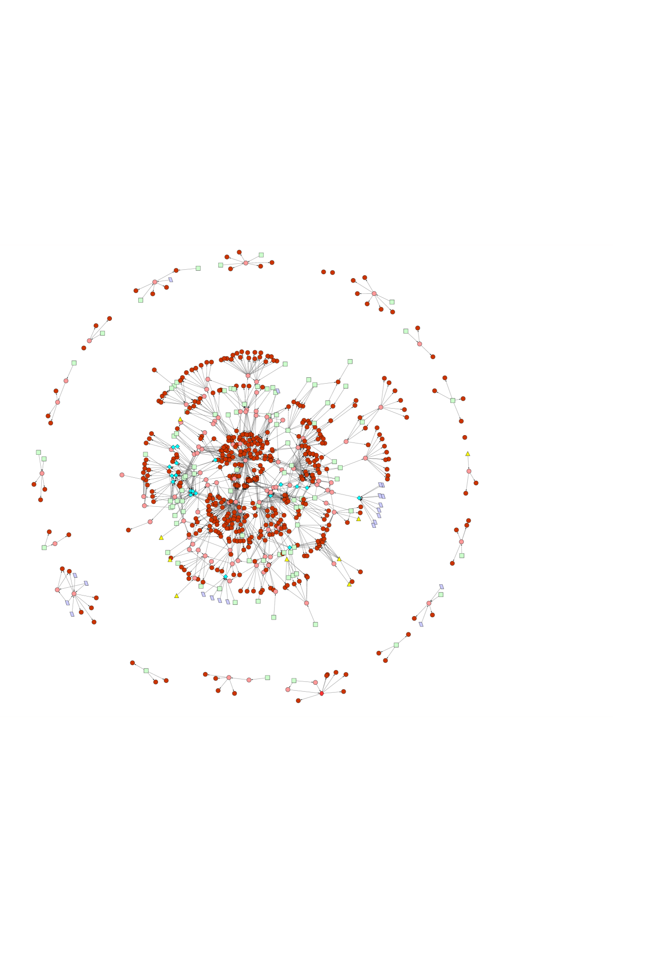
3.2 The regulatory network of E. coli metabolism as a Boolean dynamical system
We wanted to construct the simplest possible dynamical system utilizing the information regarding the network connections and regulatory logic in the database iMC1010v1 [41] to study the dynamics of the genetic network controlling E. coli metabolism. In the absence of kinetic data such as rate constants, etc., a differential equation based simulation of large scale genetic networks is not feasible at present and the large number of unknown parameters would also render the results of such a simulation difficult to interpret. Due to absence of kinetic information, the discrete time Boolean approach [57, 58, 99, 100, 59, 101, 102, 103, 104, 105, 106, 107, 108, 109] is a natural choice to study the dynamics of large scale genetic networks. Boolean simulations of smaller biological networks with a few nodes have also provided useful insights [60, 61, 62, 63, 64]. The discrete-time Boolean approach does not take into account the multiple time scales in the real system. It also does not describe large variations in concentrations as well as stochastic effects due to small numbers of molecules. Thus, the Boolean approach cannot be used for a detailed prediction of time courses and concentrations. We do not have the detailed empirical knowledge at the present time to treat these aspects of the system satisfactorily on a large scale. The Boolean approach can provide useful information about some qualitative features of the dynamics, e.g., the nature of the attractors of the system, and through that, insights regarding overall organization of the system.
We have used the information contained in the database iMC1010v1 to construct the following effective Boolean dynamical system of genes and external metabolites representing the genetic network controlling E. coli metabolism [48] (see section 3.3 for details):
| (3.1) |
Here is the configuration of gene at time . In this approach, time is taken as discrete, i.e., . Further, at any given time , a gene can be either on or off. So, = 1 (0) represents that at time gene is in on(off) state. The vector , whose component is , collectively denotes the configurations of all the 583 genes at time . The vector denotes the configuration of the 96 external metabolites in the environment. The component of vector is (). = 1 if metabolite is present in the external environment for uptake into the cell, and if metabolite is absent. The vector gives us the state of the genetic network at time and the vector represents the state of the external environment. The functions contain all the information about the internal wiring of the network (i.e., the input nodes that determine the state of gene ) as well as the Boolean logic of each gene’s regulation (i.e., given the configuration of all of gene ’s inputs at time , whether gene will be on or off at time ). Each function typically depends only upon those components of and that directly affect the expression of gene (see Fig. 3.2 for an example). Equation 3.1 expresses the fact that the on-off state of a gene at any time instant is controlled by the state of the genes at the previous time instant as well as the state of the external environment. Since the interaction of genes is mediated by transcription factors, a single time unit corresponds to the average time between the initiation of transcription of a gene coding for a transcription factor and the initiation of transcription of a gene regulated by that transcription factor. In our study, we update the state of all genes in the network synchronously. In general, note that the state of the external environment given by vector is a function of time . The concentration of metabolites in the external environment can change as the metabolic network uptakes or excretes some the metabolites across the cell boundary. However, for our study, we have considered external environment corresponding to buffered minimal media which are characterized by vectors that are constant in time. The treatment of external metabolites deciding the state of the environment is discussed in detail in section 3.3.1.
Stuart Kauffman introduced the framework of Boolean networks to study the dynamics of genetic networks about four decades ago [57, 58]. Since then Kauffman and others [57, 58, 99, 100, 59, 101, 102, 103, 104, 105, 106, 107, 108, 109] have extensively studied Boolean dynamical systems of the form:
| (3.2) |
where denotes the state of the gene at time and the vector denotes the state of all genes at time . In the above system, the state of genes is determined by only the state of other genes in the network. In the absence of detailed molecular data on real genetic regulatory networks, Kauffman and others used the Boolean approach to study biologically motivated random Boolean networks in order to gain insights about the system level dynamics of genetic networks. A random Boolean network is a system of binary nodes with inputs per node representing the regulatory mechanism. The state of any gene node at time in a random Boolean network is determined by the the state of its input nodes at previous time based on any one of the 2 possible Boolean functions with inputs. The Boolean function at each gene node is randomly chosen from the set of 2 possible Boolean functions.
Random Boolean networks have been studied extensively over the years by Kauffman and others. The study of random Boolean networks has led to several important insights regarding the dynamics of these systems. In particular, Kauffman found that random Boolean networks with large number of nodes possess an ordered regime where attractors have short periods and large basins [59]. In the ordered regime, the system was found to possess the property of homeostasis or robustness to perturbations of gene configurations. Recently, Kauffman and colleagues have also studied the Yeast regulatory network as a Boolean dynamical system where the connections between genes was based on real data while the Boolean function at each node determining the state of the gene at a given time instant based on the state of its input genes at previous time instant is randomly chosen out of a set of biologically plausible Boolean functions [105, 106]. In references [60, 61, 62, 63, 64, 110], the Boolean approach has been applied to study specific biological networks where detailed genetic data is available. These networks are smaller than the ones studied by Kauffman and colleagues, and have up to 40 distinct genes, proteins and other molecules [60, 61, 62, 63, 64, 110]. In reference [61], where a Boolean network of 180 nodes is considered, the network contains 15 distinct genes and proteins (with 12 nodes for each of them corresponding to 12 distinct cells). These models, apart from reproducing several observed phenomena of these biological systems, have also found that the networks possess the property of homeostasis, as well as robustness to genetic mutations.
This study is inspired by the work of Kauffman and extends his work in two important ways. First, it studies the genetic network controlling E. coli metabolism which has been reconstructed based on real data. The network studied here has 583 genes and 96 external metabolites which is much larger than the real biological systems studied earlier using the Boolean approach in references [60, 61, 62, 63, 64, 110]. The regulatory network contained in the database iMC1010v1 accounts for about half the genes presently believed to be involved in E. coli metabolism. The network considered here is more than an order of magnitude larger (in terms of the number of genes involved) than other real genetic networks considered as Boolean system which allows us a qualitatively different systemic view of the organization of the genetic network of an organism. Second, the present network is able to account for the effect of the external environment on the TRN dynamics through the vector in Eq. 3.1. Note that the system studied by Kauffman is described by the Eq. 3.2 instead of Eq. 3.1, which takes into account the effect of genes on other genes but not the effect of the external environment. Other works that investigated real biological systems as Boolean networks had only a few environmental signals [60, 61, 62, 63, 64, 110]. As a consequence of the database iMC1010v1, one is able to take into account the effect of external environment in a much more systematic and extensive way than before. We have studied here how the attractors of the Boolean dynamical system given by Eq. 3.1 depend upon the initial condition of the genes and the state of the external environment.
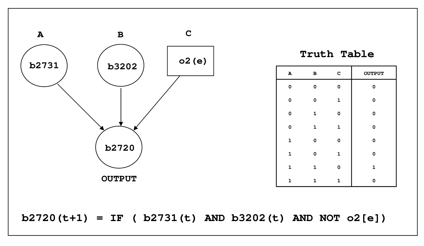
3.3 Construction of the Boolean dynamical system
We will now describe in detail the construction of the Boolean dynamical system given by Eq. 3.1 starting from the database iMC1010v1. As mentioned earlier, the database iMC1010v1 accounts for 583 genes whose state is determined by the state of 103 transcription factors, 96 external metabolites, 21 internal fluxes, 9 stimuli and 19 other conditions in the network. Further, the database iMC1010v1 gives us the Boolean input-output map for each gene node in the network in terms of the state of its input nodes. In this regulatory network, the state of various genes, transcription factors, external metabolites, internal fluxes, stimuli and conditions is represented as Boolean variables. Thus, the overall system contains 823 Boolean variables (583 genes, 103 transcription factors, 96 external metabolites, 21 internal fluxes, 9 stimuli and 19 conditions). In the present study, the 9 stimuli are assumed to be always absent. The state of the 583 genes, 103 transcription factors, 96 external metabolites, 19 conditions and 21 internal fluxes are respectively denoted by the vectors . The vectors can all in principle depend upon time . Here, (), the component of , equals unity if the gene is active or on in the cell at time and zero if the gene is inactive or off. (), the component of , equals unity if the transcription factor is present in the cell at time and zero if the transcription factor is absent. (), the component of , equals unity if the condition holds at time and zero if not. (), the component of , equals unity if the metabolic reaction in the above mentioned set of internal metabolic reactions is happening inside the cell at time (with a flux greater than a specified value) and zero if not. The state of a gene in the regulatory network at time is given by the equation:
| (3.3) |
The database iMC1010v1 gives us the form of the functions in terms of AND, OR and NOT operations on the Boolean arguments as mentioned at the end of section 3.2. The 103 transcription factors are coded for by a subset of 104 genes in the regulatory network. Of the 104 genes coding for transcription factors, 102 genes code for a single transcription factor each while two other genes together code for one transcription factor. The on-off state of the genes coding for transcription factors at the previous time instant decides the state of transcription factors at the given time instant. A single time step therefore corresponds to the average time for transcription and translation. The state of transcription factors at time is given by:
| (3.4) |
where the function
| (3.5) |
for 102 transcription factors that are coded for by single genes while for the transcription factor coded for by two genes
| (3.6) |
Substituting Eq. 3.4 in Eq. 3.3 gives us the equation
| (3.7) |
The above equation provides the dynamical rule for updating the gene configurations from one instant to the next, provided the status of the variables corresponding to external metabolites, conditions, internal fluxes, respectively, are known.
3.3.1 Treatment of external metabolites
In this study, we have considered external environment corresponding to buffered minimal media characterized by that are constant in time. For buffered media, we have
| (3.8) |
independent of time which represents a constant external environment for the cell. For each buffered medium considered, the components of m corresponding to the metabolites present in the external environment were set to unity and the remaining components were set to zero. The E. coli metabolic network iJR904 is capable of transporting 143 metabolites into and out of the cell. The 143 external metabolites in the metabolic network iJR904 include 131 organic molecules and 12 inorganic molecules. Further, 96 of the 143 external metabolites in the metabolic network iJR904 are also included in the regulatory network part of the database iMC1010v1. The 96 external metabolites accounted in the regulatory network can be divided into 86 organic molecules and 10 inorganic molecules. In this study, we have considered the following classes of minimal media:
-
(a)
List of 93 minimal media: Using the 96 external metabolites (86 organic and 10 inorganic external metabolites) contained in the regulatory network, we can construct in principle 86 aerobic and 86 anaerobic minimal media (i.e, in total 172 minimal media). A minimal medium is characterized by the availability of single organic source of carbon and the ions of ammonium, sulphate, phosphate, hydrogen, iron, potassium and sodium. The components of m corresponding to these metabolites were set to unity and others were set to zero in a given minimal medium. Oxygen was set to unity in the aerobic media and to zero in anaerobic media. FBA was performed for each of the 172 possible minimal media for the E. coli metabolic network iJR904 to obtain the optimal growth rate for each of the 172 minimal media (see Appendix B for details on FBA) . Using FBA, it was found that only 62 aerobic and 31 anaerobic minimal media supported nonzero growth. The list of 93 minimal media (62 aerobic and 31 anaerobic) is provided in Table LABEL:minimalmedialist. Note that in obtaining this list of 93 minimal media, we have used the FBA model without incorporating any regulatory constraints. We have used this list of 93 minimal media for obtaining most our results.
-
(b)
Library of 109732 media: Following Barrett et al [111], we obtained a list of 109732 media. The 143 external metabolites in the E. coli metabolic network were divided into the four different sets: carbon sources, nitrogen sources, sulphur sources and phosphorus sources. Note that the four sets are not mutually exclusive. For example, an amino acid is a carbon source as well as a nitrogen source. A large library of 109732 different media was obtained by picking a single metabolite from each of the four sets corresponding to carbon sources, nitrogen sources, sulphur sources and phosphorus sources. In addition, each media may or may not contain oxygen. Some of the work reported here uses this larger library of 109732 media.
| Serial number | Carbon Source | Abbreviation of the carbon source |
|---|---|---|
| 1 | 2-Dehydro-3-deoxy-D-gluconate | 2ddglcn |
| 2 | N-acetyl-D-glucosamine | acgam |
| 3 | L-Arabinose | arab-L |
| 4 | Cytidine | cytd |
| 5 | D-Fructose | fru |
| 6 | L-Fucose | fuc-L |
| 7 | D-Glucose 6-phosphate | g6p |
| 8 | D-Galactose | gal |
| 9 | D-Galactarate | galct-D |
| 10 | D-Galactonate | galctn-D |
| 11 | Galactitol | galt |
| 12 | D-Glucosamine | gam |
| 13 | D-Glucose | glc-D |
| 14 | D-Gluconate | glcn |
| 15 | D-Glucarate | glcr |
| 16 | L-idonate | idon-L |
| 17 | Inosine | ins |
| 18 | Lactose | lcts |
| 19 | Maltose | malt |
| 20 | Maltohexaose | malthx |
| 21 | Maltopentaose | maltpt |
| 22 | Maltotriose | malttr |
| 23 | Maltotetraose | maltttr |
| 24 | D-Mannose | man |
| 25 | Melibiose | melib |
| 26 | D-Ribose | rib-D |
| 27 | L-Rhamnose | rmn |
| 28 | D-Sorbitol | sbt-D |
| 29 | Trehalose | tre |
| 30 | Xanthosine | xtsn |
| 31 | D-Xylose | xyl-D |
| 32 | 3-(3-hydroxy-phenyl)propionate | 3hpppn |
| 33 | Acetate | ac |
| 34 | Acetoacetate | acac |
| 35 | D-Alanine | ala-D |
| 36 | L-Alanine | ala-L |
| 37 | L-Arginine | arg-L |
| 38 | L-Asparagine | asn-L |
| 39 | L-Asparate | asp-L |
| 40 | Citrate | cit |
| 41 | Fumarate | fum |
| 42 | L-Glutamine | gln-L |
| 43 | L-Glutamate | glu-L |
| 44 | Glycine | gly |
| 45 | Glycerol | glyc |
| 46 | Glycolate | glyclt |
| 47 | Hexadecanoate (n-C16:0) | hdca |
| 48 | D-Lactate | lac-D |
| 49 | L-Lactate | lac-L |
| 50 | L-Malate | mal-L |
| 51 | D-Mannitol | mnl |
| 52 | Octadecanoate (n-C18:0) | ocdca |
| 53 | Phenylpropanoate | pppn |
| 54 | L-Proline | pro-L |
| 55 | Pyruvate | pyr |
| 56 | D-Serine | ser-D |
| 57 | L-Serine | ser-L |
| 58 | Succinate | succ |
| 59 | L-tartrate | tartr-L |
| 60 | L-Threonine | thr-L |
| 61 | L-Tryptophan | trp-L |
| 62 | Tetradecanoate (n-C14:0) | ttdca |
3.3.2 Treatment of conditions
The 19 Boolean variables corresponding to conditions can be divided as follows:
-
•
15 of the 19 Boolean variables depend upon the configuration of a subset of transcription factors and external metabolites at time , i.e.,
(3.9) where the Boolean functions are given by the database iMC1010v1. The functions given by Eq. 3.9 can be substituted in Eq. 3.3 which eliminates these 15 variables from the dynamical system at the expense of more complicated effective dependence of on and .
-
•
Another condition variable corresponds to the growth of the cell. This variable representing the growth of the cell is fixed to unity as most media considered in this study give a nonzero growth rate for the cell.
-
•
Another condition variable corresponds to the pH of the external environment. In this study, pH is taken to be between 5.5 and 7, i.e., weakly acidic. For example, one of the habitats of E. coli is the human gut where the pH is weakly acidic. The pH condition affects only 3 genes in the network. For two of the genes that are affected by pH condition, the operative regulatory clause is ‘pH 4’. The Boolean variable corresponding to pH is fixed to zero (false) for these two genes. For the third gene the clause is ‘pH 7’. For this gene, the Boolean variable corresponding to pH is fixed to unity (true).
-
•
The remaining two condition variables correspond to ‘surplus FDP’ and ‘surplus PYR’ in the database iMC1010v1. They represent whether surplus amounts of fructose 1,6-bisphosphate and pyruvate are being produced in the cell. These two conditions depend upon the values of some of the internal fluxes and the presence of an external metabolite, fructose, through specified Boolean functions in the database. The variable corresponding to external fructose is treated as unity, if the minimal medium includes fructose and zero otherwise. The treatment of the internal fluxes is discussed next.
3.3.3 Treatment of internal fluxes
The state of some of the genes in the regulatory network is influenced by the state of 21 components of vector representing fluxes of internal metabolic reactions. As described in Covert et al [112], the fluxes of internal reactions in the database are surrogate for internal metabolite concentrations inside the cell that determine the state of genes in the regulatory network. The internal metabolite concentrations have been approximated by internal fluxes in the database iMC1010v1 as the database is intended to model the integrated metabolic and regulatory system f E. coli using the framework of FBA. Since FBA cannot determine the internal metabolite concentrations, the internal metabolite concentrations have been approximated by internal fluxes of reactions in the network. In this study, we have treated the variables corresponding to the internal fluxes in two distinct ways leading to two slightly different dynamical systems as discussed below.
-
(a)
System A: In the first approach, for a given external environment , we determined whether each of the 21 internal reactions in the E. coli metabolic network whose fluxes correspond to the 21 components of vector was ‘blocked’ or not [95, 75, 35]. A reaction is said to be blocked in a particular environmental condition, if under that medium no steady state flux is possible through it [95, 96, 75]. The algorithm to determine blocked reactions for a given environment is described in detail in section B.2 in Appendix B. An internal flux variable was set equal to zero for a medium (specified by vector ), if the reaction was found to be blocked for that medium, and unity otherwise. Thus, in this approach, the internal fluxes were not dynamical variables, but rather fixed parameters (albeit fixed with an eye on self-consistency).
-
(b)
System B: In the second approach, the Boolean variables corresponding to internal fluxes were allowed to be dynamical by making a simplifying assumption about their dynamics. In the metabolic network, the flux of a reaction is determined by the concentrations of the participating metabolites and the catalyzing enzymes. The enzyme concentrations are determined by the activity or state of their respective genes. In a discrete-time approximation, an enzyme is present at time if the genes coding for it were active at the previous time . Thus, the internal flux is set equal to unity if the genes coding for the enzyme catalyzing that metabolic reaction were active at the previous time , and zero otherwise. This could be done for a subset of 10 out of 21 internal reaction fluxes, since the genes of their catalyzing enzymes were part of the 583 genes in the database. Genes coding for the enzymes of the remaining 11 internal reaction fluxes were not part of the regulatory network database and hence the corresponding could not be made dynamical variables in this fashion. These latter were fixed as in part (a) for each medium by checking their blocked status for the medium under consideration. The approach (b) introduces feedbacks in the genetic regulatory network.
The above treatment defines the substitutions to be made in Eq. 3.3 for the variables and . Each component of c in Eq. 3.3 is either a specified Boolean function of , m, and , or is a suitably chosen Boolean constant. Each component of is, in turn, either a suitably chosen Boolean constant or a specified Boolean function of . The above mentioned substitutions together with Eq. 3.4 make the right hand side of Eq. 3.3 a function of only and , i.e., Eq. 3.3 reduces to
| (3.10) |
which is the same as Eq. 3.1. The functions define the final dynamical system, and include information coming from the functions , as well as the dependence of , and on and .
Note that the choices (a) and (b) for the variables yield different dynamical systems for Eq. 3.1 which we denote as system A and system B, respectively. In system B, 6 out of 583 genes have additional links from other genes in the set compared to system A. Programs implementing the two dynamical systems A and B are discussed in Appendix C.
3.4 Homeostasis: The attractor is insensitive to any perturbation of the genes
The trajectories of the Boolean dynamical system given by Eq. 3.1 depend on the initial state of the genes and the state of the environment. In this section, we investigate the dependence of the attractors on the initial condition of the genes for a given fixed environmental condition. Starting from 10000 randomly chosen initial conditions of the genes, i.e., vectors, we determined the attractors of the dynamical system A for a fixed environment corresponding to glucose aerobic minimal medium. For glucose aerobic minimal medium, the system reached a fixed point attractor for each of the 10000 initial conditions of the genes. For each of the 10000 initial conditions, the fixed point attractor was reached in a maximum of 4 time steps. Further, the same fixed point attractor was obtained for each of the 10000 initial conditions of the genes, under glucose aerobic minimal medium. This seems to suggest that a unique fixed point is the global attractor for the genetic network under glucose aerobic minimal medium regardless of the initial conditions of the genes. Examples are shown in Fig. 3.3 for glucose aerobic minimal medium for four different initial conditions of the genes. Similarly, we determined the attractors of the dynamical system A for each of the 93 buffered minimal media listed in Table LABEL:minimalmedialist starting from 10000 randomly chosen initial conditions of the genes in the network. For each of the 93 different buffered media, we found that the system reached a fixed point attractor in maximum of 4 time steps independent of the initial conditions of the genes in the network. The attractor was also determined for each of the 109732 media in the larger library mentioned in section 3.3.1 starting from a single randomly chosen initial condition of the genes. A fixed point attractor was found for each of the 109732 buffered media. In principle, there are 2583 initial conditions of the genes and one may argue that only a small amount of the state space has been sampled in these simulations. In the next chapter, an analytical argument will be presented based on the architecture of the regulatory network as to why a unique final configuration or attractor independent of the initial condition of the genes is inevitable for each fixed environment . Thus, we found that as long as the external environment remains fixed, the genetic network controlling E. coli metabolism will revert to a unique configuration of its genes after any perturbation of gene states.
The dynamical system B includes some additional links between genes compared to system A as was mentioned earlier. The attractors of the system B were obtained for each of the 93 buffered minimal media listed in Table LABEL:minimalmedialist starting from 1000 randomly chosen initial conditions of the genes for each minimal media. For system B, we obtained 36 distinct attractors (8 fixed point attractors and 28 two-cycles) for 89 of the 93 buffered minimal media. For the remaining minimal media, we obtained distinct attractors ( fixed point attractors and two-cycles). The attractor was again reached in a maximum of 4 time steps. For each of the two-cycles, it was found that most of the genes (562 to 567 out of 583) were in fact frozen in a fixed configuration, and only 16 to 21 genes oscillated back and forth between zero and one with period two. These 21 genes are listed in Table 3.2. Furthermore, for any given medium, it was found that each of the 562 frozen genes had the same configuration across all the attractors (36 or 10). This means that for any given medium, most genes (562 or more out of 583) end up in the same fixed configuration independent of the initial conditions of the genes. One can show that there are no other attractors of the system B, using the structural properties of the regulatory network. We have also checked that the 562 frozen genes end up in the same configuration in both system A and system B for any given medium.
Together, the results obtained here for dynamical systems A and B imply that the regulatory network controlling E. coli metabolism exhibits a high degree of homeostasis, in that it is highly insensitive to initial conditions of the genes. Further, for any given medium, all genetic perturbations die out very quickly, restoring an overwhelming majority of the genes to a configuration that is independent of the perturbation.
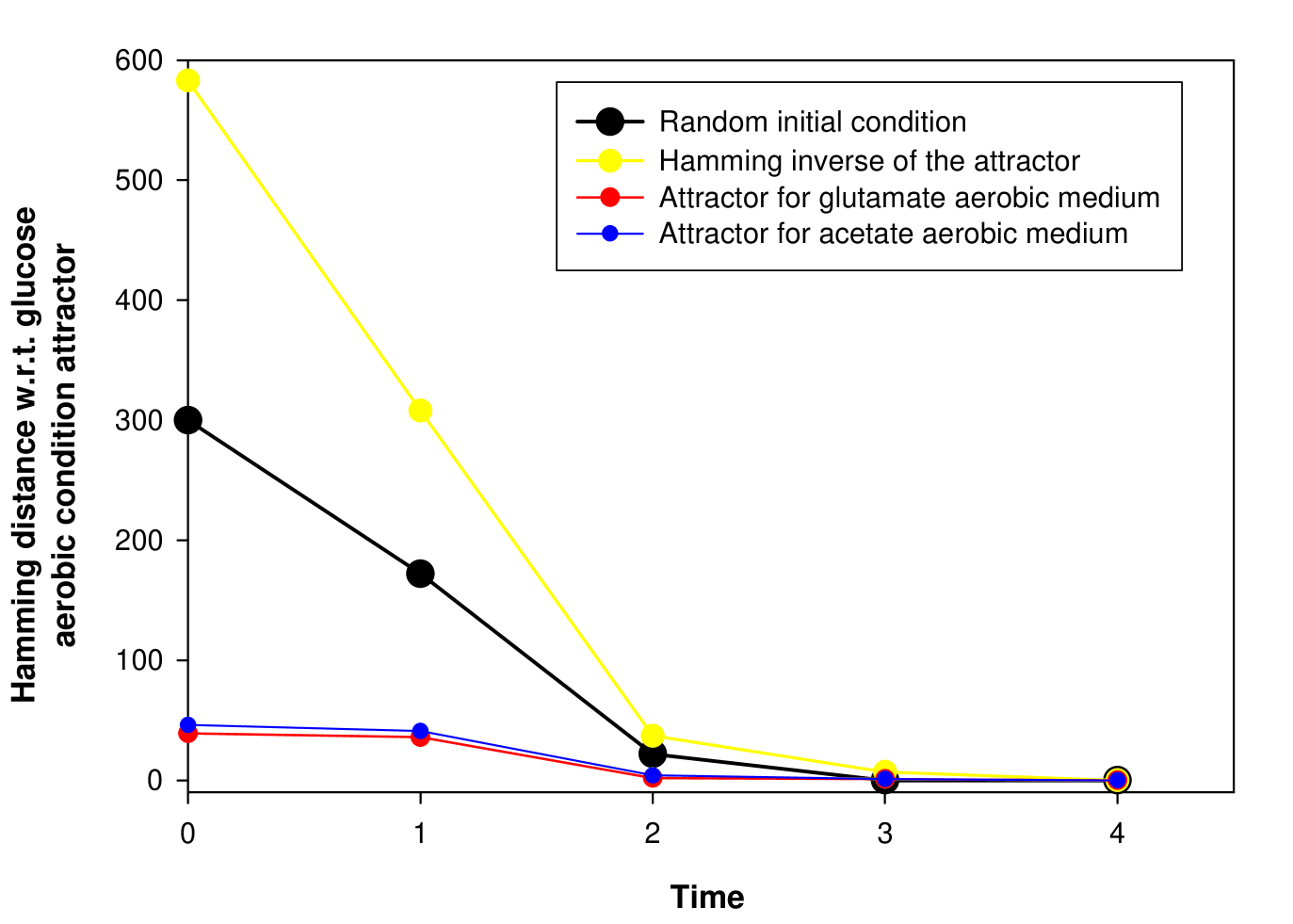
| Gene | bnumber |
|---|---|
| nagC | b0676 |
| nagA | b0677 |
| nagB | b0678 |
| nagE | b0679 |
| deoR | b0840 |
| uxaB | b1521 |
| kdgR | b1827 |
| uxaA | b3091 |
| uxaC | b3092 |
| exuT | b3093 |
| exuR | b3094 |
| kdgK | b3526 |
| glmU | b3730 |
| kdgT | b3909 |
| uxuA | b4322 |
| uxuB | b4323 |
| uxuR | b4324 |
| deoC | b4381 |
| deoA | b4382 |
| deoB | b4383 |
| deoD | b4384 |
3.5 Flexibility: The system mounts a highly flexible response to changed environments
In the last section, we have seen that the genetic network controlling E. coli metabolism exhibits the property of homeostasis or robust adaptation to internal perturbations of gene configurations for a fixed external environment. While this property of homeostasis is very useful for any given environmental condition, the organism also needs to exhibit a robust and flexible response to external perturbations corresponding to changes in the environment. In this section, we investigate the sensitivity of the attractors of the genetic network to changes in the environmental conditions. We studied the flexibility of the genetic network to environmental changes in two ways.
First, we determined the hamming distance between attractor states of the system A corresponding to pairs of minimal media. For the set of 93 buffered minimal media listed in Table LABEL:minimalmedialist, we had obtained the attractors of the system A starting from different initial conditions of the genes. The attractor was found to be a fixed point for any given minimal medium independent of initial conditions of the genes. Thus, a set of 93 fixed point attractors was obtained for the set of 93 minimal media listed in Table LABEL:minimalmedialist. We found the largest hamming distance between any two attractors out of this set for 93 minimal media to be 114.
We had also obtained the attractors of the dynamical system A for each of the 109732 media contained in the larger library mentioned in section 3.3.1. For each of the 109732 media, a fixed point attractor was obtained. We then ran ‘constrained FBA’ for each of the 109732 attractors for the larger library of 109732 buffered media to determine which of them support a nonzero growth rate for their corresponding buffered media (for details of constrained FBA, see section B.3 in Appendix B). We obtained a nonzero growth rate for the attractors corresponding to 15427 buffered media. We then computed the pairwise hamming distances among this set of 15427 attractors also. The largest hamming distance between any pair of attractors was found to be 145. The distribution of these hamming distances is trimodal as shown in Fig. 3.4. The trimodal distribution obtained here is similar to that found and discussed by Barrett et al [111]. Thus, although the attractor for a fixed environmental condition is unique, the attractors for two different environmental conditions can be quite far apart. Therefore, while the system is insensitive to fluctuations of gene configurations for a fixed external environment, it can move to quite a different attractor when it encounters a changed environment. Thus, the system shows flexibility of response to changed environmental conditions.
Second, we determined the number of media in which any gene is on across the set of attractors for 15427 buffered media. This number for any gene can range from 0 to 15427. We found that across these 15427 conditions the genes that had a configuration which differed between any pair of attractors were drawn from a set of 374 out of the 583 genes in the network. Of these 374 genes, 66 genes code for transcription factors and 308 genes code for metabolic enzymes. The remaining 209 genes had the same configuration (75 off and 134 on) in all the 15427 attractors. The variability of a gene’s configuration across different environmental conditions can be characterized by the standard deviation of its value (0 or 1) across this set. We found this standard deviation to range from zero to close to its maximum possible value 0.5. The mean of the standard deviations for the 374 genes whose configuration can differ across the set of 15427 attractors is 0.20. The histogram of standard deviation values is shown in Fig. 3.5. These observations quantify the considerable variety in a gene’s variability across environmental conditions.
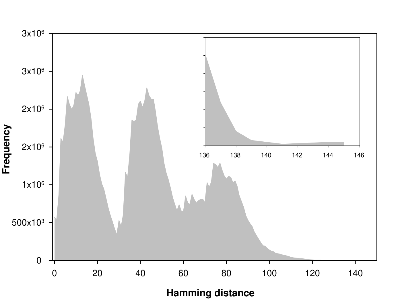
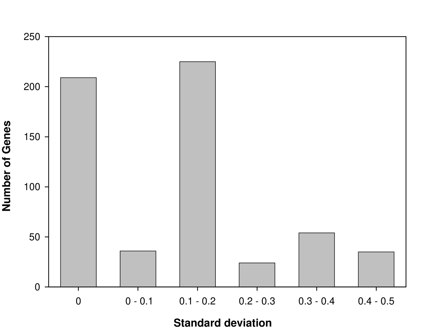
3.6 Adaptability: The regulatory network’s response to changed media increases metabolic efficiency
In this section, we tracked how the metabolic response of the cell, as measured by its growth rate computed using FBA, changes when its environment changes. A reaction in the metabolic network can be assumed to be off if none of the enzymes catalyzing it are being produced, or, equivalently, in our dynamical system, if the genes coding for those enzymes are in the off state. For any configuration of the metabolic genes, FBA can thus be used to compute the growth rate of the cell by turning off all reactions whose corresponding genes are in the off state in that configuration, thereby capturing the effect of gene regulation on metabolic function (see section B.3 in Appendix B). We computed this ‘constrained FBA’ growth rate for each of the attractors of the dynamical system A for the 93 minimal media listed in Table LABEL:minimalmedialist. 81 of them, listed in Table LABEL:optimalitytable, gave a nonzero growth rate. Starting from an initial condition of the genes in dynamical system A that corresponds to the attractor for any one of the 81 buffered minimal media listed in Table LABEL:optimalitytable, say X, we computed the time course of the genetic network configuration in another buffered medium, say Y, until the system reached the attractor corresponding to minimal medium Y. For each of the genetic network configurations in the trajectory, i.e., from the attractor for medium X to the attractor for medium Y, we computed the growth rate using constrained FBA. This effectively tracks how the constrained growth rate of the cell changes with time after its environment changes suddenly from X to Y. The result is shown in Fig. 3.6 for the cases where the carbon source in X is glutamate and in Y is glutamine, lactate, fucose or acetate. In the attractor of X the growth rate is low for the medium Y. We find that genetic network configuration changes with time so as to typically increase the growth rate.
We found that for the 81 minimal media listed in Table LABEL:optimalitytable, the growth rate in the attractor configuration of the medium was greater than the average growth rate in the other 80 attractors by a factor of 3.5 (averaged over the 81 media). Moreover, the average time to move to the attractor configuration from initial conditions corresponding to attractors for 80 remaining media was only 2.6 time steps. In other words, regulatory dynamics enables the cell to adapt to its environment to increase its metabolic efficiency very substantially, fairly quickly.
We then considered the set of 15427 media whose respective attractor configurations gave a nonzero growth rate following constrained FBA. We also computed the pure FBA growth rate for each of these 15427 media without imposing any regulatory constraints from the respective attractors for these media. We determined the ratio of the constrained FBA growth rate to the pure FBA growth rate for each of the 15427 media. The average value of this ratio was found to be as high as 0.815 and was less than 0.5 for only 7% of the media. The histogram of these ratios is shown in Fig. 3.7. This shows that the regulatory dynamics results in a close-to-optimal metabolic functioning under a large set of environments. This observation also lends support to the usefulness of FBA in probing metabolic organization.
We remark that in a dynamical system of the type given by Eq. 3.1, it is of course not surprising that the attractor of the genes’ configuration depends upon the external metabolite configuration . Our results related to flexibility and adaptability are an attempt to quantify the change in the attractors as the external environment is varied and to show that the change is functionally useful in the survival of the organism.
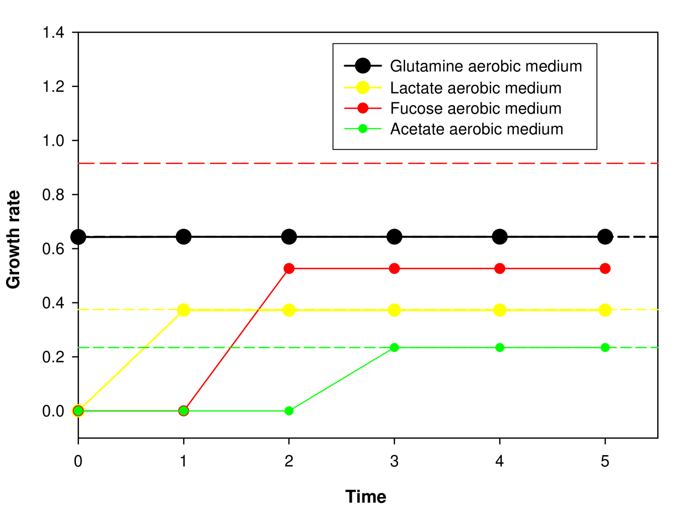
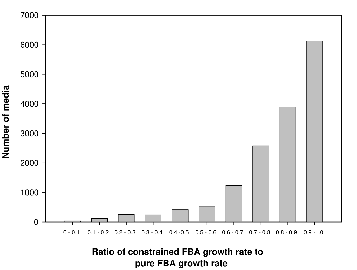
| Serial | Minimal | Oxygen | Growth Rate with | Growth Rate with no | Ratio |
|---|---|---|---|---|---|
| number | media | availability | regulatory constraints | regulatory constraints | (GRreg/GRpure) |
| (GRreg) | (GRpure) | ||||
| 1 | ac | aerobic | 0.234 | 0.234 | 0.998 |
| 2 | ala-D | aerobic | 0.416 | 0.423 | 0.985 |
| 3 | ala-L | aerobic | 0.416 | 0.423 | 0.985 |
| 4 | arab-L | aerobic | 0.785 | 0.786 | 0.998 |
| 5 | arab-L | anaerobic | 0.220 | 0.222 | 0.992 |
| 6 | arg-L | aerobic | 0.743 | 0.784 | 0.948 |
| 7 | asn-L | aerobic | 0.452 | 0.452 | 0.999 |
| 8 | asp-L | aerobic | 0.451 | 0.451 | 0.998 |
| 9 | cytd | aerobic | 0.826 | 0.872 | 0.948 |
| 10 | cytd | anaerobic | 0.282 | 0.394 | 0.716 |
| 11 | ddglcn | aerobic | 0.830 | 0.831 | 0.998 |
| 12 | ddglcn | anaerobic | 0.226 | 0.228 | 0.993 |
| 13 | fru | aerobic | 0.955 | 0.957 | 0.998 |
| 14 | fru | anaerobic | 0.297 | 0.299 | 0.992 |
| 15 | fuc-L | aerobic | 0.526 | 0.915 | 0.575 |
| 16 | fuc-L | anaerobic | 0.156 | 0.158 | 0.993 |
| 17 | fum | aerobic | 0.439 | 0.439 | 0.998 |
| 18 | g6p | aerobic | 0.990 | 0.992 | 0.998 |
| 19 | g6p | anaerobic | 0.377 | 0.380 | 0.992 |
| 20 | gal | aerobic | 0.944 | 0.946 | 0.998 |
| 21 | gal | anaerobic | 0.270 | 0.272 | 0.992 |
| 22 | galct-D | aerobic | 0.663 | 0.664 | 0.998 |
| 23 | galct-D | anaerobic | 0.209 | 0.210 | 0.993 |
| 24 | galctn-D | aerobic | 0.830 | 0.831 | 0.998 |
| 25 | galctn-D | anaerobic | 0.226 | 0.228 | 0.993 |
| 26 | galt | aerobic | 1.007 | 1.009 | 0.998 |
| 27 | galt | anaerobic | 0.253 | 0.255 | 0.993 |
| 28 | gam | aerobic | 0.955 | 0.957 | 0.998 |
| 29 | gam | anaerobic | 0.297 | 0.299 | 0.992 |
| 30 | glc-D | aerobic | 0.955 | 0.957 | 0.998 |
| 31 | glc-D | anaerobic | 0.297 | 0.299 | 0.992 |
| 32 | glcn | aerobic | 0.876 | 0.877 | 0.998 |
| 33 | glcn | anaerobic | 0.241 | 0.243 | 0.990 |
| 34 | glcr | aerobic | 0.663 | 0.664 | 0.998 |
| 35 | glcr | anaerobic | 0.209 | 0.210 | 0.993 |
| 36 | gln-L | aerobic | 0.644 | 0.644 | 0.999 |
| 37 | glu-L | aerobic | 0.670 | 0.674 | 0.994 |
| 38 | glyc | aerobic | 0.555 | 0.555 | 0.998 |
| 39 | glyclt | aerobic | 0.177 | 0.177 | 0.998 |
| 40 | hpppn | aerobic | 1.124 | 1.125 | 0.999 |
| 41 | idon-L | aerobic | 0.866 | 0.867 | 0.998 |
| 42 | idon-L | anaerobic | 0.207 | 0.208 | 0.992 |
| 43 | ins | aerobic | 0.888 | 0.889 | 0.998 |
| 44 | ins | anaerobic | 0.350 | 0.352 | 0.995 |
| 45 | lac-D | aerobic | 0.410 | 0.413 | 0.992 |
| 46 | lac-L | aerobic | 0.372 | 0.375 | 0.992 |
| 47 | lcts | aerobic | 1.900 | 1.903 | 0.998 |
| 48 | lcts | anaerobic | 0.566 | 0.571 | 0.992 |
| 49 | mal-L | aerobic | 0.427 | 0.439 | 0.971 |
| 50 | malt | aerobic | 1.911 | 1.914 | 0.998 |
| 51 | malt | anaerobic | 0.593 | 0.598 | 0.992 |
| 52 | malthx | aerobic | 5.826 | 5.835 | 0.998 |
| 53 | malthx | anaerobic | 1.995 | 2.010 | 0.992 |
| 54 | maltpt | aerobic | 4.824 | 4.832 | 0.998 |
| 55 | maltpt | anaerobic | 1.591 | 1.603 | 0.992 |
| 56 | malttr | aerobic | 2.867 | 2.871 | 0.998 |
| 57 | malttr | anaerobic | 0.890 | 0.897 | 0.992 |
| 58 | maltttr | aerobic | 3.822 | 3.828 | 0.998 |
| 59 | maltttr | anaerobic | 1.186 | 1.195 | 0.992 |
| 60 | man | aerobic | 0.955 | 0.957 | 0.998 |
| 61 | man | anaerobic | 0.297 | 0.299 | 0.992 |
| 62 | melib | aerobic | 1.900 | 1.903 | 0.998 |
| 63 | melib | anaerobic | 0.566 | 0.571 | 0.992 |
| 64 | mnl | aerobic | 1.020 | 1.025 | 0.995 |
| 65 | pro-L | aerobic | 0.754 | 0.762 | 0.990 |
| 66 | pyr | aerobic | 0.346 | 0.348 | 0.992 |
| 67 | rib-D | aerobic | 0.750 | 0.751 | 0.998 |
| 68 | rib-D | anaerobic | 0.139 | 0.140 | 0.992 |
| 69 | rmn | aerobic | 0.526 | 0.915 | 0.575 |
| 70 | rmn | anaerobic | 0.156 | 0.158 | 0.993 |
| 71 | sbt-D | aerobic | 1.020 | 1.025 | 0.995 |
| 72 | sbt-D | anaerobic | 0.256 | 0.258 | 0.992 |
| 73 | ser-D | aerobic | 0.346 | 0.348 | 0.992 |
| 74 | ser-L | aerobic | 0.354 | 0.356 | 0.994 |
| 75 | succ | aerobic | 0.469 | 0.469 | 0.998 |
| 76 | tre | aerobic | 1.911 | 1.914 | 0.998 |
| 77 | tre | anaerobic | 0.593 | 0.598 | 0.992 |
| 78 | xtsn | aerobic | 0.857 | 0.859 | 0.998 |
| 79 | xtsn | anaerobic | 0.346 | 0.348 | 0.995 |
| 80 | xyl-D | aerobic | 0.785 | 0.786 | 0.998 |
| 81 | xyl-D | anaerobic | 0.220 | 0.222 | 0.992 |
3.7 Robustness of the network to gene knockouts
In this section, we investigate the robustness of the network functionality to successive gene knockouts. We considered the progressive decline of metabolic performance for an ensemble of 1000 ‘random knockout trajectories’. Each trajectory was constructed as follows: One out of 583 genes was chosen at random and knocked out, i.e., its was set to be identically zero. The constrained FBA growth rate was then determined for the attractors of the resultant dynamical system of 582 genes for each of the 81 minimal media listed in Table LABEL:optimalitytable. If a nonzero growth rate was obtained for at least one of the 81 minimal media, we continued and knocked out another gene at random from the remaining 582 genes. This process of knocking out a randomly chosen gene from the network is repeated until the attractors for all the 81 media in the truncated network become dysfunctional (i.e., gave a zero growth rate). The number of knockout steps, , needed for the network to become metabolically dysfunctional for all the 81 media was determined for each of the 1000 random knockout trajectories considered. Figure 3.8 shows the number or frequency of trajectories with a given value of . The curve fits the exponential distribution with . Thus, we find that the chance of survival of the organism decreases exponentially with the number of gene knockouts.
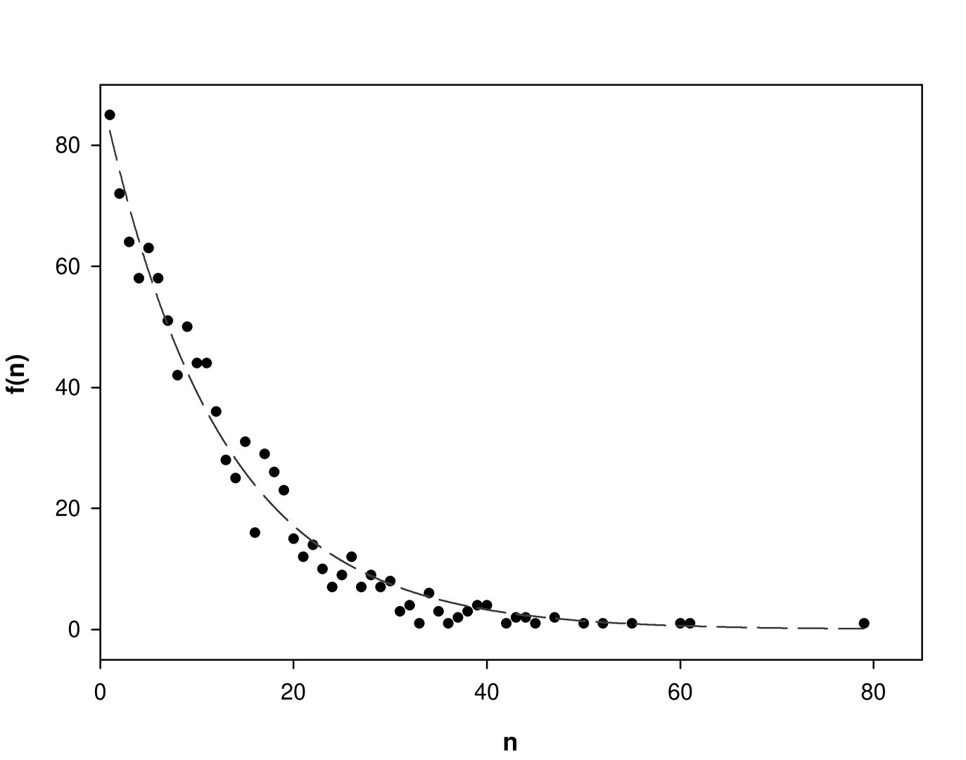
Chapter 4 Design features of the genetic network controlling E. coli metabolism
In chapter 3, we have studied the regulatory network of E. coli metabolism contained in the database iMC1010v1 [41] as a Boolean dynamical system. We found that the regulatory network of E. coli metabolism exhibits two biologically important system level properties: homeostasis and flexibility of response to changed environments. In this chapter, we explore the relationship between the structure of the genetic network controlling E. coli metabolism and the observed system level dynamical properties discussed earlier. Our study reveals that some very simple architectural features of the genetic network controlling E. coli metabolism are responsible for several of the observed system level dynamical properties.
4.1 The regulatory network of E. coli metabolism is essentially an acyclic graph
The directed graph of the regulatory network of E. coli metabolism as contained in the database iMC1010v1 was shown in Fig 3.1. In Fig. 3.1, we can see that there is a large connected component and few disconnected components. The large connected component accounts for most (86%) nodes in the regulatory network.
We found the regulatory network for dynamical system A to be an acyclic directed graph with maximal depth 4. The largest connected component of Fig. 3.1 is shown as a hierarchical inverted tree in Fig. 4.1, where all links are pointing downwards. At the bottom of the hierarchy are the nodes that have no outgoing links in the regulatory network. We refer to the nodes at the bottom of the hierarchy as ‘leaves’ of the acyclic graph. The leaves of the regulatory network are the 479 genes coding for enzymes. The largest connected component of the regulatory network shown in Fig. 4.1 has 409 genes coding for enzymes at the bottom of the hierarchy. At the top of the hierarchy are the nodes that have no incoming links in the regulatory network. We refer to the nodes at the top of the hierarchy as ‘root nodes’ of the acyclic graph. The depth of a node in the acyclic graph is the length of the longest path to it from a root node. Root nodes correspond to external metabolites and other variables that have fixed values in the dynamical system A such as internal reaction fluxes, certain conditions, etc. In our simulations of the dynamical system given by Eq. 3.1 in chapter 3, we consider only buffered media that are characterized by vector constant in time. Thus, the variables corresponding to external metabolites are held fixed for a particular simulation, and by virtue of their root location, these variables act as control variables of the dynamical system. The genes coding for transcription factors are at intermediate levels in the acyclic graph.
The above mentioned structural characteristics of the regulatory network for dynamical system A explains why
-
(a)
there are only fixed point attractors of this dynamical system,
-
(b)
their basin of attraction is the entire configuration space,
-
(c)
it takes at most 4 time steps to reach the attractors from any initial configuration, and
-
(d)
the attractor configuration depends upon the medium.
The configuration of the external environment represented by vector determines the configuration of the root level in the acyclic graph. For any fixed environment, the configuration of the root nodes are fixed. This then fixes the configurations of all nodes at the next level or depth 1 at the next time instant () and subsequent times irrespective of their values at time , because the input variables to the Boolean functions controlling them are fixed. This then fixes the configurations of all nodes at depth 2 at time irrespective of their configurations at time , and so on, until at time , the configuration of the leaf nodes at maximum depth (depth 4) are fixed irrespective of the configuration these nodes had held earlier. Thus, in 4 time steps, all nodes in the graph have reached a fixed configuration and the attractor is a fixed point. The same kind of considerations apply when we start from any arbitrary initial condition of genes as long as the configuration of the root nodes is held fixed. This implies that for a fixed external environment, starting from any initial configuration of the genes the system will reach a unique fixed point which is a global attractor. Thus, the basin of attraction is the entire configuration space of the genes.
A change in the medium or external environment is a change in the configuration of root nodes at the top of the hierarchy. The change of the configuration of root nodes percolates down the hierarchy in a maximum of 4 time steps resulting in a new fixed point attractor. Thus, the hierarchical and acyclic structure of the graph, along with external metabolites as root nodes or control variables explains the insensitivity of the attractors to initial condition or perturbation of the genes’ configuration as well as responsiveness of the attractors to changed environments.
The acyclicity of the transcriptional regulatory network of E. coli was noted earlier by Shen-Orr et al [37]. Shen-Orr et al had found that the known regulatory network of E. coli was devoid of cycles of length 2. There were only autoregulatory loops in the known regulatory network of E. coli compiled largely from RegulonDB database [36]. The autoregulatory loops are not included in the database iMC1010v1 studied here. Ma et al [46] also observed the hierarchical acyclic structure of the E. coli regulatory network. They found the maximum depth of the acyclic regulatory network to be 5. The regulatory network studied by Ma et al [46] included parts of the network that regulate systems other than metabolism. Here, we have studied the database iMC1010v1 that represents only the part of the known E. coli regulatory network that controls metabolism. Balaszi et al [47] had earlier observed that the control of the graph representing the E. coli regulatory network is in the hands of environmental signals. We remark that the acyclic structure of the E. coli regulatory network along with root control by environmental variables was noted by previous studies mentioned above. However, the present work is the first one that brings these facts about the structure of the E. coli regulatory network together to study its dynamics and elaborate upon the consequences of the observed architecture for homeostasis and response flexibility of the system.
Note that the graph of the regulatory network representing the dynamical system B is not completely acyclic. We allow the internal fluxes that affect the state of genes in the regulatory network to be dynamical in system B. Our treatment of internal fluxes in the dynamical system B effectively leads to some of the genes coding for enzymes which are leaves in the dynamical system A to have outgoing links that feedback to genes coding for transcription factors. Thus, the feedback from internal fluxes results in a few cycles in the regulatory network representing the dynamical system B. However, the feedback due to internal fluxes affect only 5 genes coding for transcription factors and 16 genes downstream of these coding for enzymes (21 genes in all). Due to the small depth and the highly disconnected structure of the regulatory network at the level of the genes coding for transcription factors in system A, the few cycles in the network of system B turn out to be short and localized. This results in the low period attractors and small ‘twinkling islands’ in the dynamics described in chapter 3 for system B. The oscillating genes are drawn from the set of 21 genes mentioned above. The rest of the 562 genes get fixed to the same configuration as in system A for any medium. Thus, in this study, we find that the genetic network regulating E. coli metabolism is largely an acyclic graph where the root control lies with environmental variables.
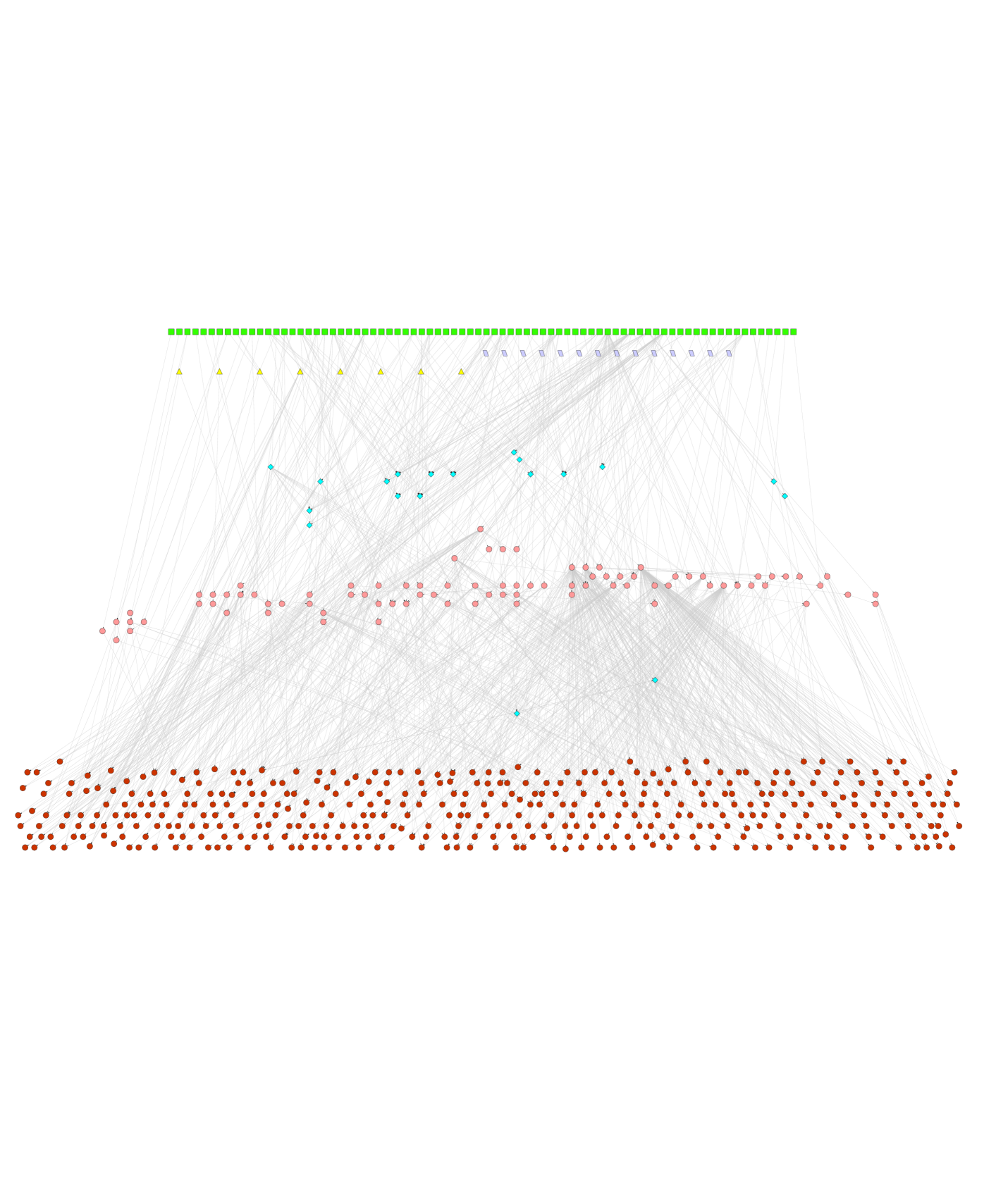
4.2 Disconnected structure of the ‘reduced dynamical system’: modularity, flexibility and evolvability
The leaf nodes corresponding to the genes coding for enzymes in the acyclic graph representing the regulatory network of E. coli metabolism have no outgoing links and their states do not determine the state of other nodes in the network. So, it is worthwhile to investigate the dynamics of the ‘reduced dynamical system’ obtained from the full system of Fig. 3.1 by removing the leaves corresponding to the enzyme coding genes at the bottom of the hierarchy. When leaf nodes in the system are removed along with all their links, we are left with Fig. 4.2 representing the reduced dynamical system. The reduced dynamical system shown in Fig. 4.2 is a disconnected graph with unexpectedly large number of disconnected components. The largest connected component of the full network shown in Fig. 4.1 has broken up into 38 disconnected components in Fig. 4.2. There are several small components containing upto only 4 nodes at depth and one component with 27 genes coding for transcription factors at depth in the reduced dynamical system. The latter component is regulated by oxygen, some inorganic sources of nitrogen, certain amino acids and sugars. The smaller components in the reduced dynamical system are typically regulated by single metabolites or groups of biochemically related metabolites. This procedure reduces the number of outgoing links for global regulators drastically. For example, the gene b3357 coding for Crp is left with only 3 outgoing links in the reduced system of Fig. 4.2 instead of 105 in the full system of Fig. 3.1.
Two components of a dynamical system that are disconnected from each other are dynamically independent as two nodes belonging to different disconnected components do not affect the states of each other. Thus, the dynamics of each disconnected component can be analyzed independent of the other disconnected components. The dynamics of the ‘reduced dynamical system’ shown in Fig. 4.2, in particular its attractors and basins of attraction, can be reconstructed from those of its disconnected components. Such a disconnected or ‘product’ structure of a dynamical system greatly simplifies its mathematical analysis. Modularity of biological systems refers to the existence of subsystems that are relatively independent of each other. We may regard each disconnected component in Fig. 4.2 as defining a core of a module. The modularity of the present genetic regulatory network is then nothing but the property that it is composed of disconnected components at this level of description.
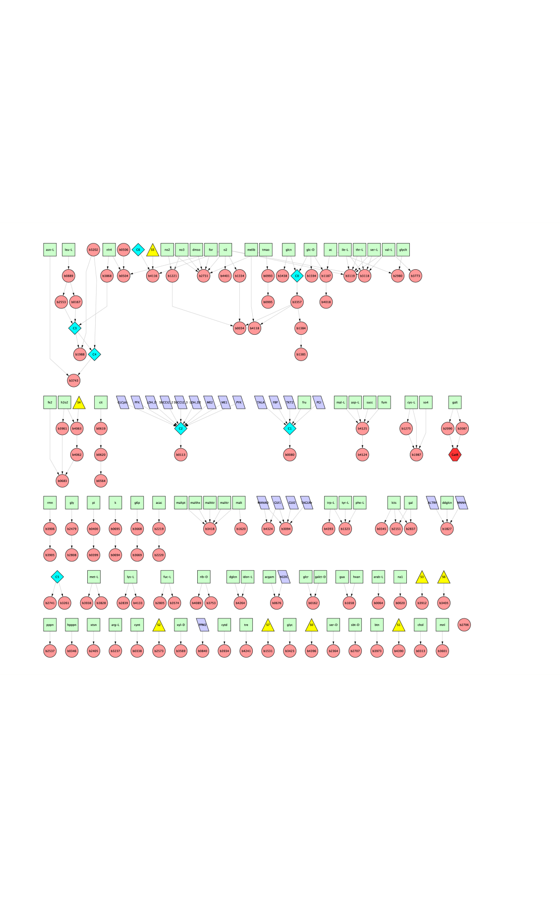
Starting from a disconnected component of Fig. 4.2 (or a module core) the genes downstream from it which code for enzymes (and do not feedback into the upper layers) may be regarded as constituting the rest of the module. Thus, a single genetic module is a disconnected component of Fig. 4.2 together with all its downstream leaves. Restoring the leaves and their links in Fig. 4.2 will take us back to Fig. 3.1 which contains the large connected component shown in Fig. 4.1. As the full system shown in Fig. 3.1 has a large connected component and a few disconnected components as opposed to many disconnected components in the reduced system shown in Fig. 4.2, this means that leaf nodes typically receive links from more than one module core of the reduced dynamical system. The structure of the acyclic graph of the regulatory network resembles that of a banyan tree which has multiple trunks emanating from independent roots and in which leaves receive sustenance from more than one root. In the present architecture, there is no direct crosstalk between the module cores of the reduced dynamical system at the level of transcription factor coding genes but the module cores can affect common leaf nodes corresponding to enzyme coding genes. This enables many leaf nodes to be influenced by several root nodes corresponding to environmental variables. This ‘multitasking’ adds to the complexity of cellular response to different environments and possibly contributes to greater metabolic efficiency. When the environment is changed from one minimal medium to another, it corresponds to replacement of one carbon source by another which may belong to a different module core of the reduced dynamical system. The genetic network needs to respond to the change of medium by activating genes coding for enzymes that catalyze metabolic reactions needed to break down the new carbon source and process its moieties. The connections of the leaf nodes to the modules above them must be such that the genes coding for enzymes catalyzing the input metabolic pathway of the new carbon source get activated, given our finding that the constrained FBA growth rate increases as the new attractor is reached (see section 3.6 in chapter 3).
The location and dynamical autonomy of the modules in the reduced dynamical system could also contribute to evolvability. If a new module is added to the reduced dynamical system of Fig. 4.2, it would not affect the dynamics of the existing modules. Thus, the organism can explore new environmental niches characterized by new food sources without jeopardizing existing capabilities. This may be a particular case of the more general observation that the architectural features of organisms responsible for their flexibility to environmental conditions also contribute to their evolvability [113, 114].
| Abbreviation | Name |
|---|---|
| C0 | CRP noGLC |
| C1 | Surplus FDP |
| C2 | Surplus PYR |
| C3 | NRI_low |
| C4 | NRI_hi |
| C5 | Growth |
| C6 | pH |
| S0 | Dipyridyl |
| S1 | High NAD |
| S2 | Heat shock |
| S3 | Stress |
| S4 | Oxidative stress |
| S5 | LBMedia |
| S6 | High osmolarity |
| S7 | Salicylate |
4.3 Almost all input functions are canalyzing in the E. coli regulatory network
Kauffman and colleagues studied extensively the dynamics of random Boolean networks in an attempt to gain understanding of the system level behaviour of real genetic regulatory networks [59]. They constructed random Boolean networks with binary nodes and inputs per node. The Boolean function that decides the state of each node at time based on the state of the input nodes at time was chosen at random from the set of possible Boolean functions of inputs in a random Boolean network. By studying random Boolean networks, Kauffman and others have found that the system can be in two different dynamical regimes: ordered and chaotic. Kauffman found that random Boolean networks with and large are deep in the ordered regime for random choice of Boolean functions. For , the random Boolean networks for random choice of Boolean functions are in the chaotic regime. Further, it was found that random Boolean networks with and large are exactly in the phase transition between the ordered and chaotic regimes for random choice of Boolean functions. It was shown that biasing the choice of Boolean functions in the generation of random Boolean networks can drive networks with into the ordered regime [59]. It has been shown by Kauffman and his colleagues that stability to perturbations in the random Boolean networks with can arise due to the canalyzing property of input functions [59, 102, 105, 106]. A canalyzing Boolean function has at least one input such that at least one of the two values of this input determines the output of the function [59]. For example, the AND, OR and NOT functions satisfy the canalyzing property while the XOR function does not satisfy the canalyzing property. For a given number of inputs, , the fraction of Boolean functions that are canalyzing decreases as increases.
On the basis of above mentioned findings, Kauffman had suggested that the distribution of Boolean functions in real genetic regulatory networks should be biased towards the set of canalyzing functions. In reference [102], Harris et al compiled Boolean rules for eukaryotes from the available literature and found all rules in their compilation to be canalyzing. For the present regulatory network of E. coli metabolism, the frequency distribution of the number of genes with regulatory inputs is given in Table 4.2. We found that Boolean functions for of the genes in the regulatory network of E. coli metabolism to possess the canalyzing property. Only genes had input functions that were not canalyzing. The above results establish the preponderance of canalyzing Boolean functions in the regulatory network of E. coli metabolism.
| Number of regulatory inputs | Number of Genes |
| 1 | 259 |
| 2 | 189 |
| 3 | 68 |
| 4 | 39 |
| 5 | 10 |
| 6 | 4 |
| 8 | 2 |
4.4 The dynamical system achieves flexibility even though it is far from the ‘edge of chaos’
As mentioned earlier, by studying extensively the dynamics of random Boolean networks, Kauffman had found that these systems can exist in two broad regimes: ordered and chaotic. In the ordered regime, the attractors of the dynamical system have a large ‘frozen core’ of genes locked in fixed configuration along with a few ‘twinkling islands’ of genes that may switch states between the two allowed values. In the chaotic regime, the number of genes in the frozen core is much less than the number of genes in the twinkling islands. One might expect that a dynamical system whose attractors have large frozen cores and very small twinkling islands is rather rigid and therefore unlikely to be adaptable to the external environment and also unlikely to be evolvable. This expectation led Kauffman to the conjecture that genetic regulatory systems ought to be close to the ‘edge of chaos’, the boundary that separates the ordered regime from the chaotic regime in the space of dynamical systems (see [59]).
However, in the previous chapter, we have shown the regulatory network of E. coli metabolism to be deep in the ordered regime, since it always falls into the same attractor that is a fixed point or has isolated low period cycles for all initial conditions of genes in a few time steps. Thus, all or most genes in the the regulatory network of E. coli metabolism get frozen for a fixed environment. In other words, the dynamical system studied by us is far from the edge of chaos. We have seen above that this property of homeostasis is an inevitable consequence of the hierarchical, largely acyclic architecture of the regulatory network. Simultaneously, we have shown in the last chapter that the system is also highly responsive to changes in the environment. How have these two properties managed to co-exist? The answer lies in the observation that root nodes of the hierarchical, acyclic graph of the regulatory network are primarily the environmental variables (i.e., the external metabolites in the present network). The attractor configuration is thus a function of the external environment, specified by the vector representing the state of the 96 external metabolites in the medium. For any fixed vector corresponding to a buffered medium, there is a global attractor in which most or all genes in the network have frozen configurations. However, when vector changes the genes ‘unfreeze’ and move to a new attractor configuration. The modular organization of the network with a lot of crosstalk between modules at the leaf level (enzyme coding genes) ensures that the melting and refreezing is quite substantial. Furthermore, the same architecture that produces this flexibility of response to the external environment can also enhance evolvability.
The present architecture as an alternative to the edge of chaos hypothesis for simultaneously producing homeostasis and flexibility has not been noticed earlier because the earlier literature has primarily focussed on the abstract genetic network itself without much reference to the environmental control variables that abound in the real systems. We have observed this architecture in the present work because the dynamical system studied here systematically accounts for the effect of external metabolites on the state of the genetic network controlling E. coli metabolism. This possibility has become evident because the database iMC1010v1 brings together, within the same network, genes as well as nodes describing external environmental signals, on a large scale.
Chapter 5 Discussion and Future Outlook
In this thesis, we have studied the large scale structure and system level dynamics of certain biological networks. Further, we have tried to explain the observed system level dynamical properties of the biological networks studied in terms of their underlying structure. In this chapter, we now summarize some of the results reported in this thesis and discuss possible implications as well as limitations associated with our work. We also mention some future directions of research and speculations based on work reported here.
5.1 Metabolic networks: low degree metabolites, essential reactions, functional modules
5.1.1 Summary of the results, discussion and speculations
In chapter 2, we have introduced the notion of ‘uniquely produced’ (‘UP’) and ‘uniquely consumed’ (‘UC’) metabolites in the metabolic network. We have designated a metabolite that is both UP and UC as a ‘UP-UC’ metabolite in the network. A UP-UC metabolite has only one reaction producing it and one reaction consuming it in the network. We have designated a set of reactions connected by UP-UC metabolites as a ‘UP-UC cluster’ in the metabolic network. Under any steady state, the flux of the reaction producing a UP-UC metabolite is proportional to the flux of the reaction consuming it. Hence, in any steady state, the fluxes of all reactions that are part of a single UP-UC cluster in the metabolic network are always proportional to each other. We have determined the list of UP(UC) metabolites and UP-UC clusters of reactions in the metabolic networks of E. coli, S. cerevisiae and S. aureus. Further, we have used the computational technique of flux balance analysis (FBA) to determine essential reactions for growth in the metabolic networks of E. coli, S. cerevisiae and S. aureus.
In chapter 2, we have shown that UP-UC metabolites in the metabolic network lead to correlated UP-UC clusters of reactions in the network. We found that large UP-UC clusters are over-represented in the real metabolic network as opposed to randomized networks with same local connectivity as the real network. We then showed that UP-UC clusters at the metabolic level correspond, with a high probability, to sets of genes forming expression modules at the regulatory level in E. coli. We have used here only the operon information in determining the correspondence between UP-UC clusters in the metabolic network and sets of coexpressed genes in regulatory network. It is possible for genes that do not belong to the same operon to be coexpressed inside the cell. Thus, an extended analysis of E. coli gene expression data may find a better correspondence between UP-UC clusters at the metabolic level and sets of coexpressed genes at the regulatory level. Further, the analysis of gene expression data to check coregulation of genes corresponding to UP-UC clusters of reactions should be extended to other organisms where operon information is not available.
Metabolic networks inside different organisms have been shown to follow a power law degree distribution [25, 28]. It has been suggested that the power law degree distribution of real networks contributes towards its robustness [33]. In particular, it has been emphasized that networks with power law degree distribution are vulnerable to selective attack on its high degree nodes or hubs, while removal of many low degree nodes from these networks have negligible effect on the functionality of the system [33]. For example, in the case of the internet, the removal of high degree nodes corresponding to routers with many connections can turn out to be fatal for the communication system. Further, for the S. cerevisiae protein-protein interaction network, the essentiality of a protein was also found to be correlated with the degree of the protein in the network [34]. However, in case of the metabolic network, the metabolites participate in reaction processes where they are produced or consumed. We can only control the reaction process through its catalyzing enzyme that is a product of some gene. It is unclear how a biological process can lead to removal of metabolites from the network. A removal of high degree metabolite from the metabolic network would require elimination of all reactions in which the metabolite participates or knockout of all genes associated with reactions in which the metabolite is involved. Further, genetic mutations effectively correspond to removal of biochemical reactions from the metabolic network. Thus, in case of the metabolic network, one is interested in determining the effect of removing a reaction rather than the effect of removing a metabolite. In chapter 2, we have shown that most globally essential reactions in the metabolic networks of E. coli, S. cerevisiae and S. aureus either produce or consume a low degree UP or UC metabolite. The essential reactions may involve other metabolites of higher degree, but their essentiality is due to their uniqueness in producing or consuming an intermediate low degree UP or UC metabolite that is needed for the eventual production of biomass. Thus, we have shown here that, in a consideration of robustness or fragility of metabolic networks to naturally occurring perturbations, it is the role of low degree metabolites that needs to be considered rather than high degree metabolites. This is an example of how the study of dynamical properties (in this case, flows) and functionality at the system level can alter one’s perspective on what is significant for robustness or fragility of real world complex systems. We remark that the importance of low degree nodes in determining the robustness or fragility of complex networks has also been observed elsewhere [115, 116]. There the crashes of an evolving catalytic network were found to be due to ‘core-shifts’ caused by changes in low degree nodes of the network.
The existence of essential reactions in the metabolic network is an indicator of the fragility in the system. Even though the metabolic networks we have studied have many reaction nodes, a small perturbation such as the removal of a single essential reaction node from the network, destroys the functionality of the complete metabolic network. One way of dealing with this fragility is by introducing redundancy at the level of genetic network by associating genes coding for isozymes with essential reactions. Isozymes are multiple enzymes catalyzing a single reaction in the metabolic network. We have to knockout multiple genes at the same time in order to remove an essential reaction with associated isozymes from the metabolic network. Hence, we may expect essential reactions in the metabolic network to have a greater probability of being associated with isozymes than non-essential reactions. However, in an earlier paper [117], Papp et al showed that both essential and non-essential reactions in the metabolic network of S. cerevisiae are equally likely to be associated with isozymes. In that paper, isozymes were found to be associated with greater probability with reactions carrying high flux rather than with essential reactions in the metabolic network [117]. This finding suggests that organisms in the course of evolution have developed redundancies in the genetic network predominantly to associate isozymes with metabolic reactions carrying high flux rather than with essential reactions in the network.
This raises the question: why has evolution tolerated the fragility associated with essential reactions? The finding that essential reactions can be tagged by UP or UC metabolites may provide some insight into this. UP or UC metabolites that participate in very few reactions perhaps do so in part because some feature of their chemical structure prohibits ready association with other molecules in nature. If so, the low degree of UP or UC metabolites is a consequence of constraints coming from chemistry. Then evolution seems to tolerate essential reactions that produce or consume such metabolites because chemistry has left it with no other choice.
Alternatively, the fragility associated with low degree metabolites may be a byproduct of some other desirable property that contributes to evolvability or robustness of the system, such as modularity. In chapter 2, we have shown that UP-UC metabolites which have low degree in the network lead to correlated clusters of reactions in the metabolic network. This raises the question: if UP-UC metabolites contribute to modularity, could it be that the evolutionary advantages of that have outweighed the disadvantage of the above mentioned fragility caused by the same low degree metabolites? Is it the case that evolution has preferred ‘chemically constrained’ low degree metabolites in spite of the fragility they cause because they contribute to modularity?
A goal in biology is to understand highly evolved biological organization in terms of simpler and more inevitable structures [118]. In chapter 2, we have presented evidence that certain regulatory modules, in particular certain operons, mirror the UP-UC structure of the metabolites whose production and consumption they regulate in E. coli. This could be an example of how the origin of certain regulatory structure can be traced to simple chemical constraints. In future, we hope to shed light on this by investigating metabolic and regulatory networks inside many other organisms.
The fragility caused by low degree metabolites in metabolic networks can have potential applications in medicine. We have observed that essential reactions are explained by UP/UC structure in three organisms. Thus, it is likely that UP/UC structure explains essential reactions in other organisms that are pathogens for humans. This generates candidate targets for therapeutic intervention. It is conceivable that drugs could be found that incapacitate the enzymes of one or the other essential reactions in pathogens.
5.1.2 Caveats regarding metabolic networks
We now discuss some limitations and caveats associated with our results reported in chapter 2. The results have been obtained by using the metabolic network databases iJR904 [66], iND750 [67] and iSB619 [68] for E. coli, S. cerevisiae and S. aureus, respectively. These databases were reconstructed using the annotated genome sequences for the three organisms and the available biochemical information in the literature. Since the annotation of the fully sequenced genomes of E. coli, S. cerevisiae and S. aureus is not yet complete, the list of reactions contained in the three metabolic network databases iJR904, iND750 and iSB619 is still incomplete.
We may expect additions to the list of biochemical reactions in the reconstructed metabolic network databases in future based on more complete annotation information. The addition of reactions to the reconstructed metabolic network databases can introduce alternate pathways for certain crucial metabolites required for the eventual production of biomass metabolites in the databases for the three organisms studied here. Thus, the introduction of alternate pathways may affect the set of essential metabolic reactions obtained using FBA for the three organisms. Similarly, the inclusion of additional reactions in the metabolic network databases would render some of the presently UP(UC) metabolites non-UP(non-UC).
In this context, it is worth noting that for the metabolic network databases as they stand, the present definition of UP(UC) metabolites allows us to establish a connection between distinct properties of the metabolic network. In chapter 2, we have shown that UP-UC metabolites lead to UP-UC clusters which are correlated sets of reactions in the metabolic network. The genes corresponding to UP-UC clusters were shown to predict regulatory modules in E. coli. We have also shown that most essential metabolic reactions are explained by their association with a UP or UC metabolite. Also, most of our results have been shown to hold for metabolic networks inside three distinct organisms. This suggests that our definition of UP(UC) metabolites and reactions does capture a certain useful pattern in the metabolic network. We remark that a reduction in the number of UP(UC) metabolites and essential reactions would only improve the correspondence of UP-UC clusters and regulatory modules described in section 2.3 and between the theoretically predicted and experimentally observed essential genes discussed in section 2.6.4.
5.2 The genetic regulatory network controlling metabolism in E. coli
5.2.1 Summary of results
In chapter 3, we have studied the genetic network controlling E. coli metabolism as represented in the database iMC1010v1 [41] as a Boolean dynamical system. We have constructed an effective Boolean dynamical system of genes and external metabolites using the information contained in the database iMC1010v1. We have studied the dependence of the attractors of the Boolean dynamical system representing the genetic network controlling E. coli metabolism to changes in initial conditions of genes and configuration of the external environment. Robustness is an inherent property of living systems which enables them to maintain their functionalities in the face of diverse perturbations [119, 120, 121]. Biological systems encounter externally induced perturbations in the form of changes in the environment and internal perturbations such as fluctuations in gene configurations. In chapter 3, we have shown that the genetic network controlling E. coli metabolism for a fixed external environment has essentially a unique attractor for the configuration of the genes regardless of the initial conditions or perturbations of gene configurations. So, we found the attractors of the dynamical system to be fixed points or low period cycles for any given fixed environmental condition and the system exhibits the property of homeostasis. However, robustness is a more general property than homeostasis which concerns itself with maintaining system functionality rather than system state. In chapter 3, we have then shown that when the dynamical system encounters a changed external environment, the system again flows and stabilizes to another unique attractor state regardless of the initial configuration of genes; however, the attractor for the changed environment may be widely separated from the attractor for the previous environment. We found the genetic network controlling E. coli metabolism as a dynamical system to be flexible to different environmental conditions as their attractors show a wide variation. In chapter 3, using the technique of FBA, we have further shown that the attractors of the genetic network for most environmental conditions allow optimal functioning of the underlying metabolic network. Thus, we have shown that the robustness of the genetic network controlling E. coli metabolism manifests itself in two different ways. When the system encounters internal perturbations in form of changes in genes’ configuration for a fixed external environment, the system returns to the present attractor. When the system encounters external perturbations in form of changed environment, the system moves to a new attractor that maintains the systems functionality in the sense of maintaining growth rate of the organism. Further, we have shown that the robust behaviour of the genetic network in moving to a different stable attractor state in response to a changed external environment also ensures metabolic efficiency for the organism.
In chapter 4, we have studied in detail the design features of the genetic network controlling E. coli metabolism in order to understand the origin of the observed system level dynamical properties of homeostasis and response flexibility. We have found the genetic network controlling E. coli metabolism as represented in the database iMC1010v1 to be hierarchical and an largely acyclic graph. Cycles where they did exist were found to be of small length and localized. The nodes with no incoming links in the genetic network are referred to as the root nodes of the hierarchy which correspond to different external metabolites. The nodes with no outgoing links in the genetic network are referred to as the leaves of the hierarchy which correspond to genes coding for metabolic enzymes. The nodes at the intermediate level of the hierarchical acyclic graph have both incoming and outgoing links in the genetic network and correspond to genes coding for transcription factors. The observed hierarchical architecture of the genetic network controlling E. coli metabolism with root control in the hands of external metabolites endows the system with the twin dynamical properties of homeostasis and response flexibility. Thus, the robust behaviour of the dynamical system has its origin in the underlying architecture or topology of the genetic network.
As mentioned above, the genetic network controlling E.coli metabolism as represented in the database iMC1010v1 lacks feedback from genes to other genes via transcription factors. The models studied originally by Kauffman [57, 59] were random Boolean networks. Those networks had substantial feedbacks between genes and hence had more complicated attractors and dynamics. One of our main results is that the genetic network controlling E.coli metabolism as a real biological system is structured (and hence departs from random networks) in such a way that it has simple attractors and dynamics. Thus, while at the abstract level the Boolean dynamical system studied by us is not very different from Kauffman’s (apart from the inclusion of the external environment), our dynamical results are quite different because the underlying network has a very different structure from the one considered by Kauffman.
In chapter 4, we have shown that removing the leaf nodes at the bottom of the hierarchy corresponding to the genes coding for metabolic enzymes along with their links from the full graph shown in Fig. 3.1 leads to a subgraph shown in Fig. 4.2 with many disconnected components. The various disconnected components shown in Fig. 4.2 are dynamically independent of each other and may be regarded as modules of the genetic network. The different disconnected components shown in Fig. 4.2 are regulated by different external metabolites. Thus, for any given environmental condition, only a subset of the disconnected components shown in Fig. 4.2 get switched on. The highly disconnected structure at the level of genes coding for transcription factors compared to the highly connected structure of the full network implies that the leaf nodes corresponding to the genes coding for metabolic enzymes get incoming links from many different disconnected components shown in Fig. 4.2. Thus, although there is a lack of crosstalk between disconnected components shown in Fig. 4.2, there is a lot of crosstalk between the modules at the leaf level, that of genes coding for metabolic enzymes in the genetic network.
In chapter 4, we have argued that the above mentioned disconnected structure at the level of genes coding for transcription factors can contribute towards the evolvability of the genetic network. Since the different disconnected components are regulated by different subsets of external metabolites in the environment, if a population of such cells encounters an environment where a particular set of external metabolites is consistently absent, then the species can discard the disconnected components regulated by these external metabolites from the genetic network without a loss of functionality with respect to other external metabolites. Conversely, if the population encounters a new set of external metabolites in a sustained manner, it can develop a new module with pathways controlled by this new set without affecting the existing functionality, thereby adapting itself to the new niche.
5.2.2 Caveats and speculations regarding regulatory networks
The results reported in chapters 3 and 4 have been obtained using the integrated regulatory and metabolic network database iMC1010v1 [41] for E. coli and there are limitations that stem from the reconstructed database itself. The database iMC1010v1 for E. coli has been reconstructed using various literature sources. The database iMC1010v1 describes the regulation of 583 genes in E. coli. Of the 583 regulated genes in the database iMC1010v1, 479 genes code for metabolic enzymes in E. coli. These 479 enzyme coding genes are a subset of the 904 enzyme coding genes associated with various reactions in the E. coli metabolic network database iJR904. Thus, the database iMC1010v1 does not describe the regulation of a large fraction of genes coding for metabolic enzymes in E. coli. In the database iMC1010v1, the set of 583 genes are regulated by a set of 96 external metabolites. In the E. coli metabolic network iJR904, there are 143 external metabolites which can be transported across the cell boundary. The set of 96 external metabolites accounted in the database iMC1010v1 are a subset of the 143 external metabolites contained in the metabolic network database iJR904. Thus, the database iMC1010v1 does not completely account for the effect of all possible external metabolites that the E. coli can uptake or excrete on the state of genes in the regulatory network. Further, the present incomplete genetic network database iMC1010v1 of 583 genes and 96 external metabolites could have many connections as false positives or false negatives, especially the latter. It is also possible that some of the Boolean rules in the database iMC1010v1 may be incorrect or incomplete due to lack of detailed experimental data for different possible environmental conditions. Hence, we expect modifications and expansion of the present database iMC1010v1 describing the genetic network controlling E. coli metabolism in the near future. This could modify our results on the dynamics of the genetic network controlling E. coli metabolism reported in this thesis.
We next ask the question: How would the future introduction of additional gene nodes and connections into the existing network database iMC1010v1 affect the results reported in this thesis? If new nodes and connections corresponding to genes coding for metabolic enzymes are added to the present database iMC1010v1, it is unlikely to affect our qualitative conclusions about the nature of attractors of the genetic network controlling E. coli metabolism significantly. The reason is that most of the genes coding for metabolic enzymes are likely to be leaves of the genetic network like the nodes at the bottom of Fig. 4.1, in which case they would have no outgoing links and would not affect the dynamics of other gene nodes in the network. However, the inclusion of genes coding for metabolic enzymes as well as additional connections to existing genes in the genetic network would add to the constraints on FBA. It would be then interesting to see the extent to which regulatory dynamics enhances metabolic efficiency in different environmental conditions for an enlarged genetic network accounting for the regulation of most genes coding for enzymes in the E. coli metabolic network.
If new nodes and connections corresponding to genes coding for transcription factors are added to the present database iMC1010v1, it can affect our qualitative conclusions about the dynamics and the nature of the attractors of the genetic network controlling E. coli metabolism. In particular, the introduction of feedback loops or cycles between genes coding for transcription factors could lead to longer cycles as attractors of the dynamical system. This is a question to be ultimately settled by more detailed knowledge of the empirical facts. Several regulatory systems with feedbacks are known, e.g., the Yeast cell-cycle network and the Drosophila segment polarity network [61, 62]. Several genes in E. coli are known to have autoregulatory self-loops [36] that are not included in the present database iMC1010v1. The introduction of autoregulatory loops in the present network could produce two-cycles at the individual nodes even at constant input. Earlier works have observed that apart from self-loops, the transcriptional regulatory network of E. coli is largely acyclic [37, 46, 47] and has a small depth of about 5. We remark that the lack of feedback from genes to other genes via transcription factors is not an assumption on our part, rather it reflects the way this biological system actually is as captured in the present database iMC1010v1 and also in other studies [37, 46, 47].
In addition to the feedback from genes to other genes via transcription factors, discussed above, there can be another kind of feedback in the genetic network controlling E.coli metabolism. This is the feedback of the concentrations of internal metabolites in the metabolic network into the genetic network. The feedback of internal metabolite concentrations could affect both the genes coding for enzymes and genes coding for transcription factors. In the database iMC1010v1, the effect of internal metabolite concentrations on the state of the genes has been approximated via fluxes of internal reactions in the metabolic network. In the present database iMC1010v1, there are 21 internal fluxes affecting the state of genes in the network. The feedback of these 21 internal fluxes from the metabolic network affect the state of only 5 genes coding for transcription factors and 16 genes downstream of these coding for metabolic enzymes in the present network. In chapter 3, we found that these 21 genes in the present network which get affected by metabolic feedback via internal fluxes may have their states undetermined across the different attractors for a given fixed environment. The state of these 21 genes can oscillate back and forth between zero and one in the two-cycle attractors obtained for any given fixed environment. This set of 21 genes in the genetic network controlling E.coli metabolism forms the twinkling island.
We may expect introduction of additional feedback from internal metabolite concentrations into the genetic network during the future network expansion. If the additional feedback from internal metabolite concentrations affect enzyme coding genes in the genetic network, then it is unlikely to change our qualitative conclusions about the observed dynamics of the system. Since the enzyme coding genes happen to be the leaf nodes of the hierarchical acyclic graph, they do not affect other nodes in the genetic network controlling E.coli metabolism. Thus, the effect of feedback from internal metabolite concentrations on to an enzyme coding gene is unlikely to affect the dynamics of other nodes in the genetic network. If the additional feedback from internal metabolite concentrations affect genes coding for transcription factors in the genetic network, then it can change our qualitative conclusions about the observed dynamics of the system. It is possible that there is a larger set of genes forming the twinkling island, and possibly longer cycles as attractors of the genetic network controlling E. coli metabolism. In chapter 4, we have shown that the genetic network controlling E. coli metabolism has a highly disconnected structure at the level of genes coding for transcription factors. This disconnected architecture of the network at the level of genes coding for transcription factors as well as the overall small depth (4) of that graph suggests that the introduction of addition feedback loops at the level of genes coding for transcription factors may only lead to cyclic attractors which are of low period and localized. We further showed that most Boolean functions in the present database iMC1010v1 satisfy the canalyzing property. These canalyzing functions may provide additional stability to the network when additional feedback loops get introduced.
The metabolic network needs to function at all times as it is responsible for utilizing the nutrients available in the external environment to produce the key molecules required for growth and maintenance of the cell. The lack of feedback between genes coding for transcription factors in the genetic network controlling E. coli metabolism observed here may be expected. However, it is known that there are many feedback loops at the level of the metabolic network where the concentration of an internal metabolite that is the end product of a metabolic pathway regulates the activity of the enzyme or the protein catalyzing the reaction at the start of the pathway. Such processes where the activity of the enzymes or proteins that are products of genes at the leaf level in the acyclic graph representing the genetic network controlling E.coli metabolism are controlled by internal metabolite concentrations are not included in the database iMC1010v1. Further, the regulation of enzyme activity by internal metabolite concentrations occurs at a much faster time scale than transcription processes inside the cell. E. coli is known to double its population in about 20 minutes in rich medium while transcriptional process inside cells occur in the order of minutes to hours. Thus, it is possible that metabolism being a functionality that needs to be active whenever food is available is largely regulated without cycles at the genetic level, with feedbacks typically entering at the level of metabolites regulating enzymes to ensure efficient functioning on a faster time scale. Feedback loops or cycles are expected in systems exhibiting explicit temporal phenomena such as cell cycle or circadian rhythms. Nevertheless it would be important to explore these questions with an enlarged database representing the genetic network controlling E.coli metabolism. We further need to check the universality of the observed architecture for the genetic network controlling E. coli metabolism in other organisms as and when an integrated metabolic and regulatory network database like iMC1010v1 becomes available for them.
In chapter 3, we have approximated the nonzero flux of an internal reaction by the activity of the gene coding for the enzyme catalyzing the reaction in the metabolic network. Hence, we have converted the metabolic feedback via internal fluxes into effective feedbacks from enzyme coding genes to other genes. This was done in order to have a simplified dynamics and a closed system of the genes alone (along with external metabolites). We remark that there exist in the literature alternative ways of treating metabolic feedback on regulation and in particular the flux variables. These include the regulatory FBA [112, 41, 65] and dynamic FBA [122, 123] in which the fluxes and the genes are dynamically coupled to each other. However, in these methods one makes an arbitrary choice of the flux vector out of many alternative flux vectors satisfying the constraints. Another method, SR-FBA [124], has been proposed that systematically accounts for multiple optimal metabolic steady states given a regulatory state. However, SR-FBA cannot be used for dynamical simulations since it only yields the various steady states for the metabolic-regulatory system. In chapter 3, our treatment of the internal fluxes is simpler compared to the above mentioned methods in that it eliminates the flux variables in favour of an effective feedback of the genes upon other genes. In the context of the present database, we believe that our broad conclusions would not change significantly because of our simplified approach to the treatment of the internal fluxes since the feedbacks from the fluxes affect only 5 genes coding for transcription factors and 16 genes downstream of these coding for enzymes, thus affecting only 21 genes out of 583. A better treatment of the feedbacks from internal metabolites than is achieved by our approach and the other approaches mentioned above requires metabolite concentrations which are difficult to compute at the present time due to the paucity of kinetic information for such large scale networks.
We end this chapter with a comment relating our results presented in chapters 3 and 4 to earlier works by Kauffman and a speculation. Kauffman [57, 59] has found biologically motivated random Boolean networks to possess multiple attractors that he has interpreted as different cell types of a multicellular organism. In chapters 3 and 4, we have studied the nature of the attractors of the genetic network regulating E. coli metabolism. Since E. coli is a prokaryote, perhaps it is not surprising that we get a much simpler picture of its genetic network exhibiting a much higher degree of order in the dynamics than the systems investigated by Kauffman. While we have shown in chapter 3 that the configuration of the genetic network regulating E. coli metabolism can settle down into different attractors, yet, unlike Kauffman, for whom different attractors were realized via different initial conditions of the genes, in our case the different attractors are realized when the control variables corresponding to external metabolites have different configurations. In chapter 3, we have shown that when the control variables are held fixed, there is none (or very little) multiplicity of attractors irrespective of the initial conditions of genes. The architecture and dynamics we have found in chapters 3 and 4 is probably quite suitable for prokaryotic lifestyle and evolution. The question remains open whether for eukaryotes and especially multicellular ones, the hypothesis that associates different cell types with different attractors of the regulatory network is valid. While that hypothesis remains an enticing possibility, it is worth noting that the simple architecture of the genetic network regulating E. coli metabolism described in detail in chapter 4 could have its uses in the eukaryotic case as well. Environmental control through the root nodes corresponding to external metabolites of the cellular attractors can itself cause a cell to differentiate into another type, the environment being determined in the multicellular case by the state of other cells in the organism. The modular structure of the the genetic network regulating E. coli metabolism at the intermediate level of the essentially acyclic graph described in chapter 4 would even permit a cell to hop through several attractors in the course of development of the organism as the environmental cues to this cell change. Such an architecture could thus contribute to developmental flexibility and, potentially, evolvability of eukaryotes as well. The multiplicity of internal attractor basins pointed out by Kauffman would be an asset in keeping the cell in its new attractor after a transient environmental cue has caused it to shift from one basin to another. It would be interesting to investigate these questions when a database similar to iMC1010v1 becomes available for a multicellular organism.
Appendix A List of UP-UC clusters in the E. coli metabolic network
The table below lists the 85 UP-UC clusters of various sizes in the E. coli metabolic network iJR904 [66]. The abbreviations of reactions and metabolites, the description of the metabolic pathway where the reaction occurs, the reaction equation and Gene-Protein-Reaction (GPR) association is taken from the database iJR904. After identifying the gene(s) for each reaction in every cluster using the GPR association, we determined which of the genes associated with a cluster are in the same operon. For a given cluster, genes in the same operon are coloured with the same shade (red, brown or pink). Furthermore, we have added information obtained using flux balance analysis (FBA) as to whether each reaction is ‘active’ or ‘inactive’. Active reactions in the E. coli metabolic network are those that were found to have a non-zero flux for at least one of the 89 flux vectors each corresponding to a different minimal medium (see section 2.5.1 in chapter 2). Inactive reactions are those that had a zero flux for all the 89 flux vectors. Reactions for which the corresponding gene name was not available in the database have been labelled as NA in the GPR association column. Of these 85 UP-UC clusters, 69 clusters are such that genes are identified for at least two distinct reactions in the cluster. The remaining 16 clusters are shaded blue.
![[Uncaptioned image]](https://cdn.awesomepapers.org/papers/06d0c751-aca3-489b-a94a-a696d66f547f/x14.png)
![[Uncaptioned image]](https://cdn.awesomepapers.org/papers/06d0c751-aca3-489b-a94a-a696d66f547f/x15.png)
![[Uncaptioned image]](https://cdn.awesomepapers.org/papers/06d0c751-aca3-489b-a94a-a696d66f547f/x16.png)
![[Uncaptioned image]](https://cdn.awesomepapers.org/papers/06d0c751-aca3-489b-a94a-a696d66f547f/x17.png)
![[Uncaptioned image]](https://cdn.awesomepapers.org/papers/06d0c751-aca3-489b-a94a-a696d66f547f/x18.png)
![[Uncaptioned image]](https://cdn.awesomepapers.org/papers/06d0c751-aca3-489b-a94a-a696d66f547f/x19.png)
![[Uncaptioned image]](https://cdn.awesomepapers.org/papers/06d0c751-aca3-489b-a94a-a696d66f547f/x20.png)
Appendix B Flux Balance Analysis (FBA)
Flux balance analysis (FBA) is a computational modelling technique that can be used to obtain a prediction for the fluxes of all reactions in the metabolic network and growth rate of the organism under the assumption of steady state without the detailed knowledge of rate constants [79, 80, 81, 82, 83, 84, 53, 85, 86, 87, 54, 55, 56, 88, 89, 66, 90, 91, 67, 92, 11]. The FBA approach has been primarily developed by Palsson group [22] and will be described here in some detail.
B.1 FBA modelling approach
B.1.1 Inputs for FBA model
-
1.
List of metabolic reactions along with stoichiometric coefficients of metabolites: The key requirement for modelling an organism’s metabolism using FBA is the list of all biochemical reactions along with stoichiometric coefficients of the involved metabolites that can happen inside the cell. The list of reactions must include all enzyme catalyzed internal reactions that can occur within the cell boundary and all transport processes across the cell boundary. The transport reactions must include both the diffusion and active transport mechanisms across the membrane. The list of reactions that can happen within a cell is largely known for many organisms due to availability of their annotated genomes and biochemical literature [22, 23, 24].
-
2.
Reversibility of reactions: Due to thermodynamic constraints certain reactions inside the cell are practically irreversible while other reactions are reversible. The net flux of a reversible reaction can be either in forward direction or backward direction for different environmental conditions. However, a reaction that is practically irreversible can have net flux in only one direction. Hence, the knowledge of reversibility of a reaction limits the allowable range of flux through a reaction.
-
3.
Flux capacity constraints: Based on limitations on the association rates of certain enzymes that catalyze reactions in the metabolic network, we can impose limitations on the maximum flux that can flow through a given reaction. Such constraints for certain reactions will limit the solution space of attainable flux distributions.
-
4.
Growth medium: In principle, an organism has the capability to uptake certain metabolites from its environment. These are the external metabolites that can be transported across the cell boundary. However, all external metabolites are not available for uptake in any given growth medium or environment. Hence, we need to define the growth medium for the organism. The growth medium essentially constrains the maximum uptake rates of various transport reactions across the cell boundary. If an external metabolite is not available for uptake in the growth medium then the maximum flux of the reaction that transports the external metabolite into the cell is set equal to 0. If an external metabolite is available for uptake in the growth medium then the flux of the reaction that transports the external metabolite into the cell is allowed to have a nonzero value.
-
5.
Biomass composition: We require the biomass composition of the organism in terms of ratios of key metabolic precursors that contribute to the unit production of biomass. The biomass composition is added to the metabolic network as a fictitious reaction. The stoichiometric coefficients of the biomass metabolites are based on experimentally derived proportions of the metabolite precursors that contribute to unit biomass production.
B.1.2 Assumptions in FBA model
-
1.
Steady state condition: The most important assumption made in the FBA modelling technique is that under any given environmental condition the organism reaches a steady state. A steady state condition is defined as one wherein the concentration of all metabolites and velocities of all reactions in the network are constant.
-
2.
Optimal metabolic functioning: The second assumption made in FBA is that the cell tries to adjust its intracellular machinery or reaction fluxes so as to maximize its growth rate or biomass production.
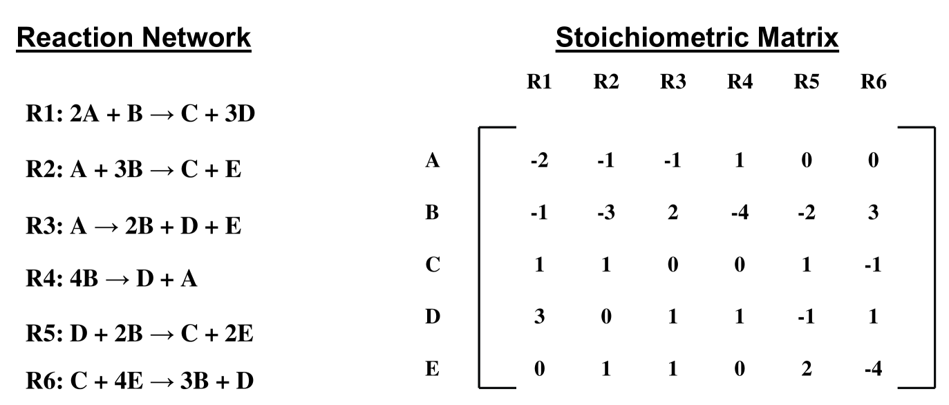
B.1.3 Computation of reaction fluxes
-
1.
Transformed network: Starting from the original reconstructed network (containing both reversible and irreversible reactions), we can obtain a transformed network by replacing each reversible reaction with two irreversible reactions (one each for the forward and backward direction). Such a transformed network has the advantage that the fluxes of all reactions in the transformed network can take only positive values, i.e.,
(B.1) where is the flux of reaction and is the number of reactions in the network. All the results presented in this thesis have been obtained using the transformed metabolic network.
-
2.
Stoichiometric matrix: The list of reactions along with the stoichiometric coefficients of the involved metabolites can be compactly represented in the form of the stoichiometric matrix. The stoichiometric matrix is a matrix of dimensions where denotes the number of metabolites and denotes the number of reactions in the metabolic network. Thus, the rows of the stoichiometric matrix correspond to various metabolites and the columns correspond to various reactions in the metabolic network. The stoichiometric matrix for a hypothetical reaction network is shown in Fig. B.1.
-
3.
Mass balance: The rate of change of concentration of a metabolite is given by the equation
(B.2) where is the concentration of metabolite , is the stoichiometric coefficient of metabolite in reaction , is the flux of reaction and is the number of reactions in the network. The above equation states that the rate of change of concentration of a metabolite is the difference between the sum of the rates at which the metabolite is produced and the sum of the rates at which the metabolite is consumed. Thus, each metabolite achieves a dynamic mass balance in the network and no mass is lost during the process. In any steady state, the above equation can be written as
(B.3) and the stoichiometric constraints can be represented by the equation
(B.4) where is the stoichiometric matrix and is the column vector representing the reaction fluxes, i.e., = (,,…,)T. In FBA, we are interested in determining the steady state flux through reactions in the metabolic network. For the metabolite A in the hypothetical reaction network shown in Fig. B.1, the steady state condition gives the equation
(B.5) where is the flux of reaction . Hence, under steady state condition, we will get a linear equation relating various fluxes for each metabolite in the network. We can determine the fluxes of reactions in the network by solving the system of linear equations relating various fluxes. However, the number of metabolites in an organism’s metabolic network is typically much less than the number of reaction fluxes to be determined. Hence, the steady state solution of reaction fluxes satisfying Eq. B.4 is underdetermined. Hence, we get a space of possible solutions satisfying the stoichiometric constraints given by Eq. B.4. The solution space can be further limited by imposing flux capacity constraints for some reactions, i.e.,
(B.6) where is the upper limit of reaction flux .
-
4.
Linear optimization: To obtain a particular solution or flux distribution from the space of possible solutions given by Eq. B.4 and flux capacity constraints for a given growth medium, linear optimization is used to find a flux distribution is the solution space that gives the optimal value for an objective function [125, 126, 127, 79, 80, 81, 82]. The most commonly used objective function is maximization of biomass production rate. Other objective functions that have been tried include maximization of ATP production and minimization of ATP utilization. Hence, one obtains a particular solution or flux distribution for a given growth medium satisfying Eq. B.4 and the flux capacity constraints such that the growth rate reaction flux has the maximum value. Some of the internal reaction fluxes and growth rate predicted using FBA for few growth media in E. coli have been shown to be consistent with experimental data [55, 56, 89].
B.1.4 Limitations of the FBA model
-
1.
Using the FBA model, we can determine only the steady state reaction fluxes in the network for a given growth medium. We cannot use the technique to predict various internal metabolite concentrations in the network.
-
2.
The regulation of metabolic reactions or pathways is completely neglected in FBA and linear optimization is used to determine the reaction or pathway flux.
-
3.
Using linear optimization, we obtain only a particular flux vector or distribution as the solution that maximizes the growth rate or biomass reaction. There are usually multiple optimal solutions that satisfy the governing constraints due to redundancies in the metabolic network [128, 129]. However, the FBA modelling approach is able to fix the value of most reaction fluxes in the network [130] and only a few reaction fluxes remain underdetermined for any given growth medium.
B.2 Blocked reactions
‘Strictly detailed balanced’ reactions [95, 96] or ‘blocked’ reactions [75] are reactions that can have only a zero flux under any steady state. The main reason for the presence of blocked reactions in various reconstructed metabolic networks is the presence of dead end internal metabolites. A dead end internal metabolite is one that either does not have a reaction consuming it or does not have a reaction producing it in the network. Since in any steady state the metabolite concentrations are constant, the sum of the fluxes of reactions producing a metabolite is equal to the sum of the fluxes of reactions consuming the metabolite. As the dead end metabolites lack either a reaction producing it or a reaction consuming it, the fluxes of reactions that involve such metabolites are guaranteed to have a zero value under any steady state. In FBA, we are interested in the steady state flux distribution for the metabolic network. The blocked reactions can be removed from the reconstructed metabolic network for any steady state analysis such as FBA. The results such as optimal growth rate and set of essential reactions obtained by implementing FBA on the original network and reduced network are the same. In this thesis, we refer to the network obtained after removing blocked reactions from the original metabolic network as the ‘reduced network’ (see also section 2.6.2 in chapter 2).
B.2.1 Algorithm to determine blocked reactions
We will now describe an algorithm previously published by Burgard et al [75] to determine blocked reactions in the metabolic
network.
Burgard et al identify reactions in the metabolic network that have their maximum and minimum flux both equal to zero for any growth
medium.
Such reactions are blocked in the metabolic network for that growth medium.
To determine blocked reactions in the metabolic network, Burgard et al solved the following linear programming (LP) problem:
Maximize flux subject to stoichiometric constraints
| (B.7) |
and flux capacity constraints
| (B.8) |
where is the stoichiometric coefficient of metabolite in reaction , is the flux of reaction that is being checked for blocked status, is the number of reactions and is the upper limit of reaction flux in the network. A reaction is said to be always blocked if the maximum flux that is obtained by solving the above mentioned LP problem is equal to zero for all possible media.
In FBA, we are interested in determining the maximum flux through the biomass reaction, given the stoichiometric constraints (Eq. B.4) and flux capacity constraints (Eq. B.6). However, while determining blocked reactions, we are interested in determining the maximum flux through the reaction being checked for blocked status, given the stoichiometric constraints and flux capacity constraints.
B.3 Constrained FBA
The state of the genetic network at any time instant is given by the configuration of its genes. In the Boolean approach, any gene in the network at a given time instant may be either active or inactive. If a gene is active, the protein coded by the gene is produced in the cell. A reaction in the metabolic network can be assumed to be off if none of the enzymes catalyzing it are being produced, or, equivalently, if the genes coding for those enzymes are in the off state. Thus, the state of the genetic network for any external environment determines the subset of reactions in the metabolic network that can happen under that condition.
In ‘pure FBA’, we leave the flux through all internal reactions unconstrained, i.e., all internal reactions are allowed to have a nonzero flux value, to determine the optimal growth rate of the cell for any given medium. Using the state of the genetic network at any time for a given medium, we can turn off all reactions whose corresponding genes are in the off state in the genetic configuration in the input to the FBA model [112]. Using FBA, we can then determine the optimal growth rate of the cell for a given medium by constraining the maximum flux through the reactions turned off by the genetic configuration to zero. This variant of FBA technique where the constraints from the state of the genetic network are incorporated to determine the growth rate of the cell may be termed as ‘constrained FBA’. Constrained FBA captures the effect of gene regulation on metabolic function. Using constrained FBA, one can track the optimal growth rate as a function of time as the configuration of the genes changes according to the dynamics of the genetic regulatory network, as also discussed earlier by Covert et al [112, 41]. One can also calculate the growth rate in the attractor configuration for any given medium. The growth rate obtained from constrained FBA for any configuration of the genes is, by definition, less than or equal to that obtained from pure FBA (for the same medium).
Appendix C Computer Programs
In this Appendix, we describe some of the computer programs used to obtain results presented in this thesis.
These programs can be downloaded from the associated website:
http://areejit.samal.googlepages.com/programs
The website contains detailed instructions to run various codes. These codes are free to use, modify and distribute for academic research. For any further queries regarding the programs contact Areejit Samal at:
areejit.samal@gmail.com
The codes mentioned below are meant for execution on any Linux Operating System. The programs have been mainly written using C++. The GNU g++ compiler was used for compiling the C++ programs. We have connected different C++ programs using shell scripts. The bash shell must be used as the default environment to run these shell scripts.
C.1 Program to determine UP-UC clusters
The C++ program UPUC.cpp can be used to determine UP-UC metabolites, UP/UC reactions and UP-UC clusters in the E. coli metabolic network iJR904. The program can be modified to determine UP-UC clusters in any metabolic network.
There are two associated input files with this program: Amatrix.txt and Metabolites.txt.
-
•
The input file Amatrix.txt contains the bipartite matrix of dimensions 618 1177 for the E. coli metabolic network iJR904.
-
•
The input file Metabolites.txt contains the list of 618 internal metabolites corresponding to rows of the bipartite matrix .
To run the program UPUC.cpp, download the three files: UPUC.cpp, Amatrix.txt and Metabolites.txt from the associated website (mentioned at the beginning of this Appendix) and put them in a single directory on a Linux system.
Compile the code by invoking the command:
g++ UPUC.cpp
followed by the instruction:
./a.out
to run the program.
The program generates the following output files: UPUCmet.txt, UPUCreac.txt and UPUCcluster.txt.
-
•
The output file UPUCmet.txt contains the UP(UC) status for each of the 618 internal metabolites in the E. coli metabolic network.
-
•
The output file UPUCreac.txt contains the UP/UC status for each of the 1176 reactions in the E. coli metabolic network.
-
•
The output file UPUCcluster.txt contains the UP-UC clusters in the E. coli metabolic network. Each line of this output file represents a single UP-UC cluster of reactions.
In addition to the three output files, the program UPUC.cpp prints out the number of UP-UC metabolites, the number of UP/UC reactions and the size distribution of UP-UC clusters in the E. coli metabolic network.
C.2 Program to determine essential reactions
The shell script Essential.sh can be used to determine essential reactions in the E. coli metabolic network iJR904 using the technique of flux balance analysis (FBA) for a specified growth medium.
The script requires the following files: glpsol, Essential.cpp, Sij.txt, Rxnlist.txt and Media.txt associated with it.
-
•
The executable file glpsol is the GNU linear programming kit solver that is used to solve the linear programming problem.
-
•
The C++ program Essential.cpp generates the MPS file for the linear programming problem to be solved.
-
•
The input file Sij.txt contains the stoichiometric matrix for the E. coli metabolic network iJR904. The dimensions of the matrix is 761 1463. The rows of the matrix correspond to metabolites and the columns correspond to reactions.
-
•
The list of 1463 reactions in the E. coli metabolic network iJR904 corresponding to the 1463 columns of the stoichiometric matrix contained in the file Sij.txt are listed in the input file Rxnlist.txt.
-
•
The input file Media.txt contains the configuration of the growth medium. At present, the growth medium is set to glucose aerobic minimal medium. The file Media.txt consists of two columns. The first column corresponds to external metabolites that the cell can uptake. The second column of the input file Media.txt corresponds to the maximum uptake rate of each external metabolite. The second column should be suitably modified to represent different growth media.
The script and its associated files can be downloaded from the associated website.
Invoke the shell script using the command:
sh Essential.sh
The program prompts you to enter the reaction to be knocked out. The program outputs the optimal growth rate of the organism for the truncated network where the reaction knocked out is absent. The steady state reaction fluxes for the truncated network is stored in the output file Flux.txt for the simulated growth medium.
C.3 Program to determine blocked reactions
The shell script Blocked.sh can be used to determine blocked status of a reaction in the E. coli metabolic network iJR904 using the algorithm by Burgard et al [75] for a specified growth medium.
The script requires the following files: glpsol, Blocked.cpp, Sij.txt, Reversible.txt and Media.txt associated with it.
-
•
The executable file glpsol is the GNU linear programming kit solver that is used to solve the linear programming problem.
-
•
The C++ program Blocked.cpp generates the MPS file for the linear programming problem to be solved.
-
•
The input file Sij.txt contains the stoichiometric matrix for the E. coli metabolic network iJR904. The dimensions of the matrix is 761 1463. The rows of the matrix correspond to metabolites and the columns correspond to reactions.
-
•
The list of 1463 reactions in the E. coli metabolic network iJR904 corresponding to the 1463 columns of the stoichiometric matrix contained in the file Sij.txt are listed in the input file Rxnlist.txt.
-
•
The list of reversible reactions in the E. coli metabolic network is contained in the input file Reversible.txt. While determining the blocked status of a reaction, we need to set the maximum flux through reactions that are exact reverse of the reaction being tested for the blocked status to zero, in order to avoid trivial cycles in the network.
-
•
The input file Media.txt contains the configuration of the growth medium. At present, the growth medium is set to be glucose aerobic minimal medium. The file Media.txt consists of two columns. The first column corresponds to external metabolites that the cell can uptake. The second column of the input file Media.txt corresponds to the maximum uptake rate for each external metabolite. The second column should be suitably modified to represent different growth media.
The script and its associated files can be downloaded from the associated website.
Invoke the shell script using the command:
sh Blocked.sh
The program prompts you to enter the reaction to be tested for blocked status. The program then outputs the maximum flux possible for the reaction being tested for blocked status under the given growth medium. If the maximum flux possible is zero, then the reaction being tested is blocked under the simulated growth medium.
C.4 Program to simulate the genetic network controlling E. coli metabolism as a Boolean dynamical system
The programs associated with the simulation of the genetic network controlling E. coli metabolism are contained in the following archive: SJ.tar.gz. Download the archive from the associated website and extract it using the command:
tar zxvf SJ.tar.gz
on a Linux operating system. The successful execution of this command will create a directory named “ECMC1010” in the current directory.
The directory ECMC1010 has two sub-directories inside it: System1A and System1B which contain the data and programs for the two dynamical systems A and B, respectively.
C.4.1 Dynamical system A
Inside the directory System1A, there are two sub-directories DATA and PROG.
-
•
In the directory DATA, the file ENV.txt gives a list of variables whose values remain fixed at all times for a given initial configuration of genes and minimal medium considered. There are 128 such variables: 1 to 96 are the external metabolites, 97 to 117 are the 21 fluxes, then the two conditions corresponding to pH and Growth, followed by the 9 stimuli which are set to be always absent in our study. We need to determine the column vector of 128 boolean variables (in the order mentioned in the file ENV.txt) for a given minimal medium to determine the attractor of the dynamical system.
-
•
We study mostly the system under the 93 minimal media, which are listed in the file MinMedia contained in directory DATA. Each line of the file MinMedia corresponds to a different minimal medium.
-
•
We fix the 21 fluxes variables for a given medium based on their blocked reaction status for that medium. For the 93 minimal media listed in the file MinMedia the information about blocked status for each of the 21 fluxes is contained in the file FLUX1Aminmedia contained in directory DATA. Here each column of the file FLUX1Aminmedia contains the blocked status information for the 21 fluxes for the minimal medium mentioned at the corresponding line of the file MinMedia. If a reaction flux is blocked for a given medium then it is set as 0 else 1. The fluxes represented in the 21 rows of the file FLUX1Aminmedia are in the same order as in the file ENV.txt.
-
•
For example, the 23rd line of file MinMedia is glucose aerobic minimal medium (see file glcaermedia) and hence the 23rd column of FLUX1Aminmedia file contains the blocked status information for the 21 fluxes for the glucose aerobic minimal medium (see file glcaerFLUX).
-
•
The system contains 583 genes and we need to start with some initial condition for the 583 genes. There are in principle possible initial conditions of genes. One possible initial condition is contained in the file INITIAL in the directory DATA.
-
•
The genes corresponding to each line of the file INITIAL are contained in the file TRNgenes in the directory DATA.
The program env.cpp in PROG directory is used to determine the vector of 128 fixed variables for a given medium. Compile the program using the command:
g++ PROG/env.cpp
Run the program as follows:
./a.out File1 File2 File3
Here,
-
•
File1 is a file containing the external metabolites in the minimal medium, i.e., one of the lines of the file MinMedia.
-
•
File2 should contain the column corresponding to the minimal medium of File1 in the file FLUX1Aminmedia, i.e., blocked reaction status of the 21 fluxes for the minimal medium studied.
-
•
File3 is the output file that will store the vector of 128 variables.
File1, File2 and File3 are command line arguments and can take any string as a name.
The program GP1A.cpp contained in the folder PROG is used to determine which proteins or transcription factors (TF) are on/off given the configuration of genes at the previous time instant.
Compile the program using the command:
g++ PROG/GP1A.cpp
Run the program as follows:
./a.out File1 File2
Here,
-
•
File1 should contain the configuration of 583 genes at the previous time instant. It can be DATA/INITIAL.
-
•
File2 is the output file containing the state of transcription factors at current time instant. The lines in the output file File2 correspond to transcription factors listed in the file TF in directory DATA.
Given the state of transcription factors at the current time instant (calculated using GP1A.cpp) and the fixed values of 128 variables for the simulated minimal medium (calculated using env.cpp), we can use TRN1A.cpp in the PROG directory to calculate the state of the 583 genes at the next time instant.
Compile the program using the command:
g++ PROG/TRN1A.cpp
Run the program as follows:
./a.out File1 File2 File3
Here,
-
•
File1 should contain the state of the transcription factors at the current time instant given the state of the genes at previous time instant.
-
•
File2 should contain the values of the 128 fixed variables.
-
•
File3 is the output file in which state of the 583 genes at the current time instant is stored.
We have connected these programs using a shell script attractor.sh which can be used to compute the attractor for a given minimal medium and initial configuration of genes. The shell script attractor.sh is contained in the directory System1A. The shell script first starts with the initial configuration of genes and a defined minimal medium and computes the state of the 583 genes for the next 200 time steps. Then a small perl script, attractor.pl in the PROG directory, is invoked to determine the attractor of the system. We are assuming here that the system reaches the attractor in 200 time steps.
Run the shell script using the command:
sh attractor.sh File1 File2 File3 File4
where,
-
•
File1 should contain the minimal medium.
-
•
File2 should contain the blocked status of 21 fluxes for the minimal medium in File1.
-
•
File3 should contain the initial configuration of genes.
-
•
File4 is the output file where the attractor is stored.
For example, run the script as follows:
sh attractor.sh DATA/glcaermedia DATA/glcaerFLUX DATA/INITIAL steady.txt
The output is stored in the file steady.txt, i.e., it contains the attractor for the glucose aerobic minimal medium for the initial configuration of genes specified in the file DATA/INITIAL.
If the attractor is of period 1, i.e., a fixed point, then this vector is contained in a line of the output file steady.txt. If the attractor is of period 2, i.e., a two cycle, then the two vectors are contained in two lines of the output file steady.txt.
There are some other files in the directory DATA:
-
•
TRN1A.txt gives the rules for the update of each of the 583 genes.
-
•
GP1A.txt gives the Gene Protein association for transcription factors in the model.
-
•
Condition1A.txt gives the rules for 17 out of the 19 conditions. The remaining two conditions, pH and Growth, are set using the program env.cpp.
In these files, stands for the NOT operator, for the AND operator and for the OR operator.
C.4.2 Dynamical system B
Inside the directory System1B, there are two sub-directories DATA and PROG.
-
•
In the directory DATA, the file ENV.txt gives a list of variables whose values remain fixed at all times for a given initial configuration of genes and minimal medium considered. There are 118 such variables: 1 to 96 are the external metabolites, 97 to 107 are the 11 fluxes, then the two conditions corresponding to pH and Growth, followed by the 9 stimuli which are set to be always absent in our study. We need to determine the column vector of 118 boolean variables (in the order mentioned in the file ENV.txt) for a given minimal medium to determine the attractor.
-
•
We study mostly the system under the 93 minimal media, which are listed in the file MinMedia contained in directory DATA. Each line of the file MinMedia corresponds to a different minimal medium.
-
•
We fix the 11 fluxes variables for a given medium based on their blocked reaction status for that medium. For the 93 minimal media listed in the file MinMedia the information about blocked status for each of the 11 fluxes is contained in the file FLUX1Bminmedia contained in directory DATA. Here each column of the file FLUX1Bminmedia contains the blocked status information for the 11 fluxes for the minimal medium mentioned at the corresponding line of the file MinMedia. If a reaction flux is blocked for a given medium then it is set as 0 else 1. The fluxes represented in the 11 rows of the file FLUX1Bminmedia are in the same order as in the file ENV.txt.
-
•
For example, the 23rd line of file MinMedia is glucose aerobic minimal medium (see file glcaermedia) and hence the 23rd column of FLUX1Bminmedia file contains the blocked status information for the 11 fluxes for the glucose aerobic minimal medium (see file glcaerFLUX).
-
•
The system contains 583 genes and we need to start with some initial condition for the 583 genes. There are in principle possible initial conditions of genes. One possible initial condition is contained in the file INITIAL in the directory DATA.
-
•
The genes corresponding to each line of the file INITIAL are contained in the file TRNgenes in the directory DATA.
The program env.cpp in PROG directory is used to determine the vector of 118 fixed variables for a given medium. Compile the program using the command:
g++ PROG/env.cpp
Run the program as follows:
./a.out File1 File2 File3
Here,
-
•
File1 is a file containing the external metabolites in the minimal medium, i.e., one of the lines of the file MinMedia.
-
•
File2 should contain the column corresponding to minimal medium of File1 in the file FLUX1Bminmedia, i.e., blocked reaction status of the 11 fluxes for the minimal medium studied.
-
•
File3 is the output file that will store the vector of 118 variables.
File1, File2 and File3 are command line arguments and can take any string as a name.
The program GP1B.cpp contained in the folder PROG is used to determine which proteins or transcription factors (TF) are on/off given the configuration of the genes at the previous time instant.
Compile the program using the command:
g++ PROG/GP1B.cpp
Run the program as follows:
./a.out File1 File2
Here,
-
•
File1 should contain the configuration of the 583 genes at the previous time instant. It can be DATA/INITIAL.
-
•
File2 is the output file containing the state of the transcription factors at the current time instant. The lines in the output file File2 correspond to transcription factors listed in the file TF in directory DATA.
Given the state of the transcription factors at the current time instant (calculated using GP1B.cpp) and the fixed values of 118 variables for minimal medium (calculated using env.cpp), we can use TRN1B.cpp in the PROG directory to calculate the state of the 583 genes at the next time instant.
Compile the program using the command:
g++ PROG/TRN1B.cpp
Run the program as follows:
./a.out File1 File2 File3
Here,
-
•
File1 should contain the state of the transcription factors at the current time instant given the state of the genes at previous time instant.
-
•
File2 should contain the values of the 118 fixed variables.
-
•
File3 is the output file in which state of the 583 genes at the current time instant is stored.
We have connected these programs using a shell script attractor.sh which can be used to compute the attractor of the system for a given minimal medium and initial configuration of genes. The shell script attractor.sh is contained in the directory System1B. The shell script first starts with a initial configuration of genes and a defined minimal medium and computes the state of the 583 genes for the next 200 time steps. Then a small perl script, attractor.pl in the PROG directory, is invoked to determine the attractor. We are assuming here that the system reaches the attractor in 200 time steps.
Run the shell script using the command:
sh attractor.sh File1 File2 File3 File4
where,
-
•
File1 should contain the minimal medium.
-
•
File2 should contain the blocked status of 11 fluxes for the minimal medium in File1.
-
•
File3 should contain the initial configuration of genes.
-
•
File4 is the output file where the attractor is stored.
For example, run the script as follows:
sh attractor.sh DATA/glcaermedia DATA/glcaerFLUX DATA/INITIAL steady.txt
The output is stored in the file steady.txt, i.e., it contains the attractor for the glucose aerobic minimal medium for the initial configuration of genes specified in the file DATA/INITIAL.
If the attractor is of period 1, i.e., a fixed point, then this vector is contained in a line of the output file steady.txt. If the attractor is of period 2, i.e., a two cycle, then the two vectors are contained in two lines of the output file steady.txt.
There are some other files in the directory DATA:
-
•
TRN1B.txt gives the rules for the update of each of the 583 genes.
-
•
GP1B.txt gives the Gene Protein association for transcription factors and enzymes in the model.
-
•
Condition1B.txt gives the rules for 17 out of the 19 conditions. The remaining two conditions, pH and Growth, are set using the program env.cpp.
In these files, stands for the NOT operator, for the AND operator and for the OR operator.
References
- [1] Watts DJ, Strogatz SH: Collective dynamics of ‘small-world’ networks. Nature 1998, 393:440–442.
- [2] Jain S, Krishna S: Autocatalytic sets and the growth of complexity in an evolutionary model. Phys Rev Lett 1998, 81:5684–5687.
- [3] Barabasi AL, Albert R: Emergence of scaling in random networks. Science 1999, 286:509–512.
- [4] Strogatz SH: Exploring complex networks. Nature 2001, 411:268–276.
- [5] Albert R, Barabasi AL: Statistical mechanics of complex networks. Rev Mod Phys 2002, 74:47–97.
- [6] Bornholdt S, Schuster HG: Handbook of Graphs and Networks: from the Genome to the Internet. Wiley-VCH 2003.
- [7] Hartwell LH, Hopfield JJ, Leibler S, Murray AW: From molecular to modular cell biology. Nature 1999, 402:C47–C52.
- [8] Kitano H: Computational systems biology. Nature 2002, 420:206–210.
- [9] Alon U: Biological Networks: The Tinkerer as an Engineer. Science 2003, 301:1866–1867.
- [10] Barabasi AL, Oltvai ZN: Network biology: Understanding the cell’s functional organization. Nat Rev Genet 2004, 5:101–113.
- [11] Palsson BO: Systems Biology: Properties of Reconstructed Networks. Cambridge University Press 2006.
- [12] Alon U: An Introduction to Systems Biology: Design Principles of Biological Circuits. Chapman & Hall 2007.
- [13] Alm E, Arkin AP: Biological networks. Curr Opin Struct Biol 2003, 13:193–202.
- [14] Bray D: Molecular networks: the top-down view. Science 2003, 301:1864–1865.
- [15] Babu MM, Lucsombe N, Gerstein M, Teichmann S: Structure and evolution of gene regulatory networks. Curr Opin Struc Biol 2004, 14:283–291.
- [16] Mangan S, Alon U: Structure and function of the feed-forward loop network motif. Proc Natl Acad Sci USA 2003, 100:11980–11985.
- [17] Guet C, Elowitz M, Hsing W, Leibler S: Combinatorial synthesis of genetic networks. Science 2002, 296:1466–1470.
- [18] Barkai N, Leibler S: Robustness in simple biochemical networks. Nature 1997, 387:855–857.
- [19] Bhalla US, Iyenger R: Emergent properties of networks of biological signaling pathways. Science 1999, 283:339–340.
- [20] von Dassow G, Meir E, Munro EM, Odell GM: The segment polarity network is a robust developmental module. Nature 2000, 406:188–192.
- [21] Kacser H, Burns JA: The control of flux. Symp Soc Exp Biol 1973, 25:65–104.
- [22] UCSD Systems Biology Research Group: http://gcrg.ucsd.edu/.
- [23] KEGG Database: http://www.genome.jp/kegg/.
- [24] Ecocyc Database: http://ecocyc.org/.
- [25] Jeong H, Tombor B, Albert R, Oltvai ZN, Barabasi AL: The large-scale organization of metabolic networks. Nature 2000, 407:651–654.
- [26] Harary F: Graph Theory. Addison-Wesley Publishing Company 1969.
- [27] Bollobas B: Random Graphs. Academic Press 1985.
- [28] Wagner A, Fell DA: The small world inside large metabolic networks. Proc R Soc Lond B 2001, 268:1803–1810.
- [29] Ma HW, Zeng AP: The connectivity structure, giant strong component and centrality of metabolic networks. Bioinformatics 2003, 19:1423–1430.
- [30] Broder A, Kumar R, Maghoul F, Raghavan P, Rajagopalan S, Stata R, Tomkins A, Wiener J: Graph structure in the web. Computer Networks 2000, 33:309–320.
- [31] Csete M, Doyle J: Bow ties, metabolism and disease. Trends Biotechnol 2004, 22:446–450.
- [32] Arita M: The metabolic world of Escherichia coli is not small. Proc Natl Acad Sci USA 2004, 101:1543–1547.
- [33] Albert R, Jeong H, Barabasi AL: Error and attack tolerance of complex networks. Nature 2000, 406:378–382.
- [34] Jeong H, Mason SP, Barabasi AL, Oltvai ZN: Lethality and centrality in protein networks. Nature 2001, 411:41–42.
- [35] Samal A, Singh S, Giri V, Krishna S, Raghuram N, Jain S: Low degree metabolites explain essential reactions and enhance modularity in biological networks. BMC Bioinformatics 2006, 7:118.
- [36] RegulonDB Database: http://regulondb.ccg.unam.mx/.
- [37] Shen-Orr S, Milo R, Mangan S, Alon U: Network motifs in the transcriptional regulation network of Escherichia coli. Nat Genet 2002, 31:64–68.
- [38] Lee TI, Rinaldi NJ, Robert F, Odom DT, Bar-Joseph Z, Gerber GK, Hannett NM, Harbison CT, Thompson CM, Simon I, Zeitlinger J, Jennings EG, Murray HL, Gordon DB, Ren B, Wyrick JJ, Tagne JB, Volkert TL, Fraenkel E, Gifford DK, Young RA: Transcriptional regulatory networks in Saccharomyces cerevisiae. Science 2002, 298:799–804.
- [39] Guelzim N, Bottani S, Bourgine P, Kepes F: Topological and causal structure of the yeast transcriptional regulatory network. Nat Genet 2002, 31:60–63.
- [40] Lucsombe N, Babu MM, Yu H, Snyder M, Teichmann S, Gerstein M: Genome analysis of regulatory network dynamics reveals large topological changes. Nature 2004, 431:308–312.
- [41] Covert MW, Knight EM, Reed JL, Herrgard MJ, Palsson BO: Integrating high-throughput and computational data elcidates bacterial networks. Nature 2004, 429:92–96.
- [42] Milo R, Shen-Orr S, Itzkovitz S, Kashtan N, Chklovskii D, Alon U: Network Motifs: Simple Building Blocks of Complex Networks. Science 2002, 298:824–827.
- [43] Ronen M, Rosenberg R, Shraiman BI, Alon U: Assigning numbers to the arrows: Parameterizing a gene regulation network by using accurate expression kinetics. Proc Natl Acad Sci USA 2002, 99:10555–10560.
- [44] Conant GC, Wagner A: Convergent evolution of gene circuits. Nat Genet 2003, 34:264–266.
- [45] Wagner A: Does Selection Mold Molecular Networks? Science Signaling 2003, pe:41–43.
- [46] Ma HW, Buer J, Zeng AP: Hierarchical structure and modules in the Escherichia coli transcriptional regulatory network revealed by a new top-down approach. BMC Bioinformatics 2004, 5:199.
- [47] Balazsi G, Barabasi AL, Oltvai ZN: Topological units of environmental signal processing in the transcriptional regulatory network of Escherichia coli. Proc Natl Acad Sci USA 2005, 102:7841–7846.
- [48] Samal A, Jain S: The regulatory network of E. coli metabolism as a Boolean dynamical system exhibits both homeostasis and flexibility of response. BMC Systems Biology 2008, 2:21.
- [49] Alon U, Surette MG, Barkai N, Leibler S: Robustness in bacterial chemotaxis. Nature 1999, 397:168–171.
- [50] Yi TM, Huang Y, Simon MI, Doyle J: Robust perfect adaptation in bacterial chemotaxis through integral feedback control. Proc Natl Acad Sci USA 2000, 97:4649–4653.
- [51] Ingolia NT: Topology and robustness in the Drosophila segment polarity network. PLoS Biol 2004, 2:e123.
- [52] Bornholdt S: Less Is More in Modeling Large Genetic Networks. Science 2005, 310:449–450.
- [53] Varma A, Palsson BO: Stoichiometric flux balance models quantitatively predict growth and metabolic by-product secretion in wild-type Escherichia coli W3110. Appl Environ Microbiol 1994, 60:3724–3731.
- [54] Edwards JS, Palsson BO: The Escherichia coli MG1655 in silico metabolic genotype: its definition, characteristics, and capabilities. Proc Natl Acad Sci USA 2000, 97:5528–5533.
- [55] Edwards JS, Ibarra RU, Palsson BO: In silico predictions of Escherichi coli metabolic capabilities are consistent with experimental data. Nat Biotechnol 2001, 19:125–130.
- [56] Ibarra RU, Edwards JS, Palsson BO: Escherichi coli K-12 undergoes adaptive evolution to achieve in silico predicted optimal growth. Nature 2002, 420:186–189.
- [57] Kauffman SA: Metabolic stability and epigenesis in randomly constructed genetic nets. J Theor Biol 1969, 22:432–467.
- [58] Kauffman SA: Homeostasis and differentiation in random genetic control networks. Nature 1969, 224:177–178.
- [59] Kauffman SA: Origins of Order: Self-Organization and Selection in Evolution. Oxford University Press 1993.
- [60] Sanchez L, Thieffry D: A logical analysis of the Drosophila gap-gene system. J Theor Biol 2001, 211:115–141.
- [61] Albert R, Othmer HG: The topology of the regulatory interactions predicts the expression pattern of the segment polarity genes in Drosophila melanogaster. J Theor Biol 2003, 223:1–18.
- [62] Li F, Long T, Lu Y, Ouyang Q, Tang C: The yeast cell-cycle network is robustly designed. Proc Natl Acad Sci USA 2004, 101:4781–4786.
- [63] Espinosa-Soto C, Padilla-Longoria P, Alvarez-Buylla ER: A gene regulatory network model for cell-fate determination during Arabidopsis thaliana flower development that is robust and recovers experimental gene expression profiles. Plant Cell 2004, 16:2923–2939.
- [64] Li S, Assmann SM, Albert R: Predicting essential components of signal transduction networks: A dynamic model of guard cell abscisic acid signaling. PLoS Biol 2006, 4(10):e312.
- [65] Herrgard MJ, Lee BS, Portnoy V, Palsson BO: Integrated analysis of regulatory and metabolic networks reveals novel regulatory mechanisms in Saccharomyces cerevisiae. Genome Res 2006, 16:627–635.
- [66] Reed JL, Vo TD, Schilling CH, Palsson BO: An expanded genome-scale model of Escherichia coli K-12 (iJR904 GSM/GPR). Genome Biol 2003, 4:R54.1–R54.12.
- [67] Duarte NC, Herrgard MJ, Palsson BO: Reconstruction and validation of Saccharomyces cerevisiae iND750, a fully compartmentalized genome-scale metabolic model. Genome Res 2004, 14:1298–1309.
- [68] Becker SA, Palsson BO: Genome-scale reconstruction Staphylococcus aureus N315: an initial draft to the two-dimensional annotation. BMC Microbiol 2005, 5:8.
- [69] Graphviz: http://www.graphviz.org/.
- [70] Pfeiffer T, Sanchez-Valdenebro I, Nuno JC, Montero F, Schuster S: METATOOL: for studying metabolic networks. Bioinformatics 1999, 15:251–257.
- [71] Schuster S, Klamt S, Weckwerth W, Moldenhauer F, Pfeiffer T: Use of network analysis of metabolic systems in bioengineering. Bioprocess Biosyst Eng 2002, 24:363–372.
- [72] Stelling J, Klamt S, Bettenbrock K, Schuster S, Gilles ED: Metabolic network structure determines key aspects of functionality and regulation. Nature 2002, 420:190–193.
- [73] Papin JA, Price ND, Palsson BO: Extreme pathway lengths and reaction participation in genome-scale metabolic networks. Genome Res 2002, 12:1889–1900.
- [74] Reed JL, Palsson BO: Genome-scale in silico models of E. coli have multiple equivalent phenotypic states: assessment of correlated reaction subsets that comprise network states. Genome Res 2004, 14:1797–1805.
- [75] Burgard AP, Nikolaev EV, Schilling CH, Maranas CD: Flux coupling analysis of genome-scale metabolic network reconstructions. Genome Res 2004, 14:301–312.
- [76] Kannan R, Tetali P, Vempala S: Simple Markov-chain algorithms for generating bipartite graphs and tournaments. Random Structures and Algorithms 1999, 14:293–308.
- [77] Maslov S, Sneppen K: Specificity and stability in topology of protein networks. Science 2002, 296:910–913.
- [78] Milo R, Itzkovitz S, Kashtan N, Levitt R, Shen-Orr S, Ayzenshtat I, Sheffer M, Alon U: Superfamilies of Evolved and Designed Networks. Science 2004, 303:1538–1542.
- [79] Savinell JM, Palsson BO: Optimal selection of metabolic fluxes for in vivo measurement. I. Development of mathematical methods. J Theor Biol 1992, 155:201–214.
- [80] Savinell JM, Palsson BO: Optimal selection of metabolic fluxes for in vivo measurement. I. Application to Escherichia coli and hybridoma cell metabolism. J Theor Biol 1992, 155:215–242.
- [81] Varma A, Palsson BO: Metabolic capabilities of Escherichia coli: I. Synthesis of biosynthetic precursors. J Theor Biol 1993, 165:477–502.
- [82] Varma A, Palsson BO: Metabolic capabilities of Escherichia coli: II. Optimal growth patterns. J Theor Biol 1993, 165:503–522.
- [83] Varma A, Boesch BW, Palsson BO: Biochemical production capabilities of Escherichia coli. Biotechnol Bioeng 1993, 42:59–73.
- [84] Varma A, Boesch BW, Palsson BO: Stoichiometric interpretation of Escherichia coli glucose catabolism under various oxygenation rates. Appl Environ Microbiol 1993, 59:2465–2473.
- [85] Varma A, Palsson BO: Metabolic flux balancing: Basic concepts, scientific and practical use. Bio/Technology 1994, 12:994–998.
- [86] Pramanik J, Keasling JD: Stoichimetric model of Escherichia coli metabolism: incorporation of growth-rate dependent biomass compostion and mechanistic energy requirements. Biotechnol Bioeng 1997, 56:398–421.
- [87] Pramanik J, Keasling JD: Effect of Escherichia coli biomass composition on central metabolic fluxes predicted by a stoichiometric model. Biotechnol Bioeng 1998, 60:230–238.
- [88] Schilling CH, Covert MW, Famili I, Church GM, Edwards JS, Palsson BO: Genome-scale metabolic model of Helicobacter pylori 26695. J Bacteriol 2002, 184:4582–4593.
- [89] Segre D, Vitkup D, Church GM: Analysis of optimality in natural and perturbed metabolic networks. Proc Natl Acad Sci USA 2002, 99:15112–15117.
- [90] Forster J, Famili I, Fu P, Palsson B, Nielsen J: Genome-scale reconstruction of the Saccharomyces cerevisiae metabolic network. Genome Res 2003, 13(2):244–253.
- [91] Kauffman KJ, Prakash P, Edwards JS: Advances in flux balance analysis. Curr Opin Biotechnol 2003, 14:491–496.
- [92] Almaas E, Kovacs B, Vicsek T, Oltvai ZN, Barabasi AL: Global organization of metabolic fluxes in the bacterium Escherichia coli. Nature 2004, 427:839–843.
- [93] Singh S, Jain S: unpublished.
- [94] Mahadevan R, Palsson BO: Properties of Metabolic Networks: Structure vs. Function. Biophys J 2005, 88:L7–L9.
- [95] Schuster S, Schuster R: Detecting strictly detailed balanced subnetworks in open chemical reaction networks. J Math Chem 1991, 6:17–40.
- [96] Heinrich R, Schuster S: The Regulation of Cellular Systems. Chapman & Hall 1996.
- [97] Gerdes SY, Scholle MD, Campbell JW, Balazsi G, Ravasz E, Daugherty MD, Somera AL, Kyrpides NC, Anderson I, Gelfand MS, Bhattacharya A, Kapatral V, D’Souza M, Baev MV, Grechkin Y, Mseeh F, Fonstein MY, Overbeek R, Barabasi AL, Oltvai ZN, Osterman AL: Experimental determination and system level analysis of essential genes in Escherichia coli MG1655. J Bacteriol 2003, 184:152–164.
- [98] Cytoscape: http://www.cytoscape.org/.
- [99] Thomas R: Boolean formalisation of genetic control circuits. J Theor Biol 1973, 42:565–583.
- [100] Derrida B, Weisbuch G: Evolution of overlaps between configurations in random Boolean networks. J Physique 1986, 47:1297–1303.
- [101] Bornholdt S, Sneppen K: Neutral mutations and punctuated equilibrium in evolving genetic networks. Phys Rev Lett 1998, 81:236–239.
- [102] Harris SE, Sawhill BK, Wuensche A, Kauffman SA: A model of transcriptional regulatory networks based on biases in the observed regulation rules. Complexity 2002, 7:23–40.
- [103] Shmulevich I, Dougherty ER, Kim S, Zhang W: Probabilistic Boolean Networks: A Rule-based Uncertainty Model for Gene Regulatory Networks. Bioinformatics 2002, 18(2):261–274.
- [104] Aldana-Gonzalez M, Coppersmith S, Kadanoff LP: Perspectives and problems in nonlinear science, A celebratory volume in honor of Lawrence Sirovich, Springer, New York 2003 chap. Boolean Dynamics with Random Couplings.
- [105] Kauffman SA, Peterson C, Samuelsson B, Troein C: Random Boolean network models and the yeast transcriptional network. Proc Natl Acad Sci USA 2003, 100:14796–14799.
- [106] Kauffman SA, Peterson C, Samuelsson B, Troein C: Genetic networks with canalyzing Boolean rules are always stable. Proc Natl Acad Sci USA 2004, 101:17102–17107.
- [107] Serra R, Villani M, Agostini L: On the dynamics of random Boolean networks with scale-free outgoing connections. Physica A 2004, 339:665–673.
- [108] Klemm K, Bornholdt S: Stable and unstable attractors in Boolean networks. Phys Rev E 2005, 72:055101.
- [109] Greil F, Drossel B: Dynamics of Critical Kauffman Networks under Asynchronous Stochastic Update. Phys Rev Lett 2005, 95:048701.
- [110] Braunewell S, Bornholdt S: Superstability of the yeast cell-cycle dynamics: Ensuring causality in the presence of biochemical stochasticity. J Theor Biol 2007, 245:638–643.
- [111] Barrett CB, Herring CD, Reed JL, Palsson BO: The Global Transcriptional Regulatory Network for Metabolism in Escherichia coli Exhibits Few Dominant Functional States. Proc. Natl. Acad. Sci. USA 2005, 102(52):19103–19108.
- [112] Covert MW, Schilling CH, Palsson BO: Regulation of Gene Expression in Flux Balance Models of Metabolism. J Theor Biol 2001, 213:73–78.
- [113] Ancel LW, Fontana W: Plasticity, Evolvability, and Modularity in RNA. J Exp Zool 2000, 288:242–283.
- [114] Kirschner MW, Gerhart JC: The Plausibility of Life: Resolving Darwin’s Dilemma. Yale University Press 2005.
- [115] Jain S, Krishna S: Crashes, recoveries and core shifts in a model of evolving networks. Phys Rev E 2002, 65:026103.
- [116] Jain S, Krishna S: Large extinctions in an evolutionary model: The role of innovation and keystone species. Proc Natl Acad Sci USA 2002, 99:2055–2060.
- [117] Papp B, Pal C, Hurst LD: Metabolic network analysis of the causes and evolution of enzyme dispensability in yeast. Nature 2004, 439:661–664.
- [118] Morowitz HJ: A theory of biochemical organization, metabolic pathways, and evolution. Complexity 1999, 4:39–53.
- [119] Stelling J, Sauer U, Szallasi Z, Doyle III FJ, Doyle J: Robustness of cellular functions. Cell 2004, 118:675–685.
- [120] Kitano H: Biological robustness. Nat Rev Genet 2004, 5:826–837.
- [121] Wagner A: Robustness and Evolvability in Living Systems. Princeton University Press 2005.
- [122] Mahadevan R, Edwards JS, Doyle FJ: Dynamic Flux Balance Analysis of Diauxic Growth in Escherichia coli. Biophys J 2002, 83:1331–1340.
- [123] Luo RY, Liao S, Tao GY, Li YY, Zeng S, Li YX, Luo Q: Dynamic analysis of optimality in myocardial energy metabolism under normal and ischemic conditions. Mol Sys Biol 2006, 2:31.
- [124] Shlomi T, Eisenberg Y, Sharan R, Ruppin E: A genome-scale computational study of the interplay between transcriptional regulation and metabolism. Mol Sys Biol 2007, 3:101.
- [125] Papoutsakis ET: Equations and calculations for fermentations of butyric acid bacteria. Biotechnol Bioeng 1984, 26:174–187.
- [126] Fell DA, Small JA: Fat synthesis in adipose tissue. An examination of stoichiometric constraints. J Biochem 1986, 238:781–786.
- [127] Majewski RA, Domach MM: Simple constrained optimization view of acetate overflow in E. coli. Biotechnol Bioeng 1990, 35:731–738.
- [128] Lee S, Phalakornkule C, Domach MM, Grossmann IE: Recursive MILP model for finding all alternate optima in LP models for metabolic networks. Comp Chem Eng 2000, 24:711–716.
- [129] Phalakornkule C, Lee S, Zhu T, Koepsel R, Ataai MM, Grossmann IE, Domach MM: A MILP based flux alternative generation and NMR experimental design strategy for metabolic engineering. Metab Eng 2001, 3:124–137.
- [130] Klamt S, Schuster S: Calculating as many fluxes as possible in underdetermined metabolic networks. Mol Biol Rep 2002, 29:243–248.
Acknowledgements
I would like to thank Prof. Sanjay Jain and Prof. Shobhit Mahajan under whose guidance the work reported in this thesis was completed.
I thank Prof. Sanjay Jain for suggesting the questions addressed in this thesis. The work reported in this thesis has been done in close collaboration with him. He introduced me to the area of complex networks and systems biology. I have learned the subject from him through numerous scientific discussions we had in the last five years. He has through his actions influenced my personality and outlook.
I would like to thank Prof. Shobhit Mahajan for always being there for me. He has been very patient to take care of my problems and encouraged me. He has also shown a lot of faith and confidence in me. I am indebted to him for his help during M.Sc. Physics. His critical comments and practical advice have helped me immensely. He has been a pillar of strength in my life.
I thank Shalini Singh, Varun Giri, Dr. Sandeep Krishna and Dr. N. Raghuram for discussions and collaborations. The work reported in Chapter 2 has been done in collaboration with them. I would also like to thank Dr. Sandeep Krishna, Shalini Singh and Varun Giri for developing the flux balance analysis (FBA) program used by our group. The program has been used for obtaining various results in this thesis.
I thank Shalini and Varun for their friendship and help. We went together to many conferences in India. I enjoyed their company during these trips. I would like to thank Varun for spending a lot of his time everyday speculating on various matters with me and keeping our discussions lively.
I would like to thank Aditya, Amit, Anubhav, Gagandeep, Utkarsh and Vinay for discussions and their questions. It was a learning experience for me while they were doing their projects with Prof. Sanjay Jain.
I thank Prof. Amitabha Mukherjee for being part of my Ph.D. advisory committee and for discussions.
I would like to thank all the members of Department of Physics and Astrophysics, University of Delhi, who have helped me during M.Sc. and Ph.D. programme. In this regard, I would like to thank Prof. S. Annapoorni, Prof. Debajyoti Choudhury, Prof. Patrick Das Gupta, Dr. Nivedita Deo, Dr. R. S. Kaushal, Dr. Daksh Lohiya, Dr. Awadhesh Prasad, Dr. T. R. Seshadri and Dr. Poonam Silotia for their help. I would like to thank Mrs. M. Dawar for facilitating various administrative matters.
I would like to especially thank Prof. D. S. Kulshreshtha for his affection, encouragement and help during the past six years.
I would like to thank Council of Scientific and Industrial Research (CSIR), Government of India for Junior Research Fellowship (JRF) (2003 - 2005) and Senior Research Fellowship (SRF) (2005 -). In this regard, I would like to thank my senior and dear friend Md. Naimuddin for his tips that were instrumental in cracking the CSIR UGC JRF(NET) examination the very first time during my Masters.
I would like to thank Prof. Ram Ramaswamy for chairing my CSIR JRF to SRF evaluation. I also thank him for various discussions and encouragement. I would like to thank Dr. Ravi Mehrotra for chairing my CSIR SRF extension evaluation and discussions.
I would like to thank Prof. Bernhard Palsson and Dr. Jennifer Reed for kindly providing the GPR association of the E. coli metabolic network iJR904. I also thank all past and present members of the Palsson group for making their reconstructions of metabolic and regulatory networks freely available to the scientific community through their website http://gcrg.ucsd.edu/. Without the availability of these reconstructed networks, the work reported in this thesis would not be possible.
I would like to thank Prof. Uri Alon for encouraging me during a conference held at NCBS, Bangalore in December 2003. The discussions I had with him helped me in deciding the problems to pursue.
In the past five years, I have visited various universities and research institutions in India. I thank Himachal Pradesh University, IISc Bangalore, IIT Kanpur, NCBS Bangalore, SNBNCBS Kolkata, and University of Pune for their hospitality and infrastructural support. I would like to also thank Dr. Kanury Rao, ICGEB, Delhi and all his group members for the opportunity to spend two months in their lab.
During my Ph.D., I have also been very fortunate to visit various research groups outside India working in the area of complex networks. In this regard, I would like to thank Dr. Johannes Berg (University of Koln), Dr. Oliver Ebenhoh (Max Planck Institute for Molecular Plant Physiology, Potsdam), Dr. Alessandro Giuliani (ISS, Rome), Prof. Hanspeter Herzel (Humboldt University, Berlin), Prof. Herrmann-Georg Holzhutter (Charite, Humboldt University, Berlin), Prof. Juergen Jost (Max Planck Institute for Mathematics in the Sciences, Leipzig), Prof. Francois Kepes (Genopole, Evry), Dr. Konstantin Klemm (University of Leipzig), Prof. Matteo Marsili (ICTP, Trieste), Prof. Olivier Martin (LPTMS, Orsay), Prof. Hildegard Meyer-Ortmanns (Jacobs University, Bremen), Dr. Jari Saramaki (HUT, Helsinki), Prof. Stefan Schuster (University of Jena), Prof. Frank Schweitzer (ETH, Zurich), Prof. Roberto Serra (European Center for Living Technology, Venice) Prof. Andreas Wagner (University of Zurich) and Dr. Martin Weigt (ISI, Torino) for their kind support. I would like to also thank all the group members of the above mentioned scientists for their hospitality during my visits.
I also had a chance to attend a lot of conferences and schools where I was unable to follow most of the talks. But this time was the most fruitful as I made a lot of friends in various scientific institutions. I would like to thank Akhilesh, Amitabha, Arnab, Bhaswar, Bino, Brojen, Dharmendra, Dhiraj, Dipanjan, Florian, Jeremiah, Johannes, Julien, Moin, Niko, Rajat, Rajesh, Ramachandran, Shilpi, Sonika, Srikanth, Sudhanshu, Vaibhao, Viren, Vishal and Vivek for all the good times.
In the last ten years, I have spent most of my time in the University of Delhi, North Campus. I wish to thank Amit, Gaurav, Geetanjali, Harish, Jaswant, Jiten, Keshwarjit, Kopal, Manish, Pooja, Pranav, Sandip, Sanil, Sunil, Sushil, Uddipan, Umeshkanta, Varun, Vikrant, Vikas, Wasim and Yogesh for their company.
I wish to especially thank Jiten for his friendship, help and encouragement during the past seven years. I am grateful to him for getting me to focus in life during M.Sc. Physics. He has always inspired me by his intelligence, modesty and generosity.
During the past five years, I have realized that Ph.D. time is full of confusions and tensions. It is very easy to make mistakes and give up under certain situations. In such situations, you need a patient, mature and understanding friend. During the last four years, I have found such a friend in Pranav.
Due to interdisciplinary nature of my work, it becomes very essential that you have friends from other fields of science with whom you can discuss your research, get suggestions and criticisms. In the last two years, I had many such stimulating discussions with Dhiraj.
In the end, I want to mention that in spite of all my shortcomings, my parents still continue to sacrifice their life for me and love me more and more with each passing day.
Areejit Samal