Subband Splitting: Simple, Efficient and Effective Technique for Solving Block Permutation Problem in Determined Blind Source Separation
Abstract
Solving the permutation problem is essential for determined blind source separation (BSS). Existing methods, such as independent vector analysis (IVA) and independent low-rank matrix analysis (ILRMA), tackle the permutation problem by modeling the co-occurrence of the frequency components of source signals. One of the remaining challenges in these methods is the block permutation problem, which may cause severe performance degradation. In this paper, we propose a simple and effective technique for solving the block permutation problem. The proposed technique splits the entire frequency bands into several overlapping subbands and sequentially applies BSS methods (e.g., IVA, ILRMA, or any other method) to each subband. Since the splitting reduces the size of the problem, the BSS methods can effectively work in each subband. Then, the permutations among the subbands are aligned by using the separation result in one subband as the initial values for the other subbands. Additionally, we propose SS-IVA and SS-ILRMA by combining subband splitting (SS) with IVA and ILRMA. Experimental results demonstrated that our technique remarkably improves the separation performance without increasing computational cost. In particular, our SS-ILRMA achieved the separation performance comparable to the oracle method (frequency-domain independent component analysis with the ideal permutation solver). Moreover, SS-ILRMA converged faster than conventional IVA and ILRMA.
1 Introduction
Determined blind source separation (BSS) is a technique for separating the source signals from multichannel observed signals. It is usually formulated as an optimization problem of the demixing matrices in the time-frequency domain. To separate the signals with this formulation, addressing the permutation problem is essential. Namely, the order of extraction target must be kept consistent across all frequencies[1, 2]. While a permutation solver[3, 4, 5, 6, 7, 8, 9] is required in frequency-domain independent component analysis (FDICA)[1, 2], later methods, e.g., independent vector analysis (IVA)[10, 11, 12, 13, 14, 15, 16, 17, 18, 19, 20, 21, 22], independent low-rank matrix analysis (ILRMA)[23, 24, 25, 26, 27, 28, 29, 30], and those assisted by deep learning [31, 32, 33, 34, 35, 36, 37, 38], model the co-occurrence of the frequency components and align the permutation within the optimization algorithms.
Although these methods can align the permutation to some extent, they sometimes fail due to block permutation problem[16, 28, 29, 8, 36]. That is, several frequency blocks with inconsistent permutations may arise and cause severe performance degradation. To deal with the block permutation problem, the following three types of approaches have been employed in many existing methods. The first one utilizes an external permutation solver tailored for block permutation problem[29, 8]. The second one incorporates spatial information (e.g., the directions of the sources) into BSS algorithms[28, 21, 22]. The last approach is to improve the source models. In particular, aiming to precisely model the frequency-band-wise structures of the sources, several methods incorporated subband structures into the source model of IVA and ILRMA[16, 17, 18, 19, 20, 30]. These three approaches have mitigated the block permutation problem. However, some of these methods may require additional computational costs for external solvers (the first approach), while others may require efforts to develop optimization algorithms, especially when incorporating more sophisticated source models (the second and third approaches).
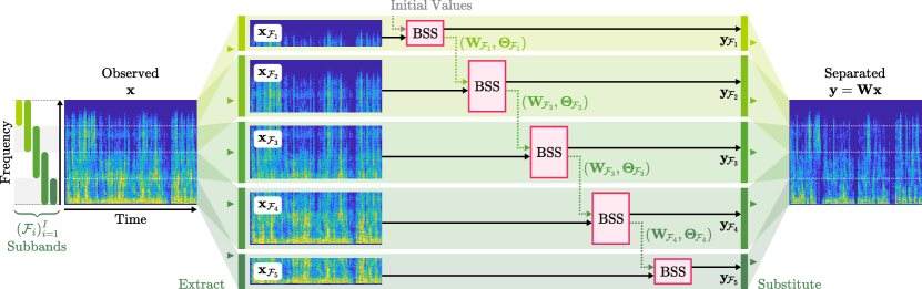
In this paper, we propose a simple technique named subband splitting (SS) to enhance the separation performance of existing BSS algorithms111 The same proposal has already been uploaded on arXiv[39] . As illustrated in Fig. 1, our technique splits the entire frequency bands into several overlapping subbands and then sequentially applies BSS algorithms to each subband. Owing to the splitting, the size of the optimization problem in each subband is reduced, and therefore source separation can be more easily done. Then, the separation results from one subband are used to initialize BSS algorithms in the subsequent subbands, which aligns the permutations across all subbands. Notably, our technique does not require any modification to the BSS algorithms nor additional computational cost. Therefore, it can be directly combined with various BSS algorithms and can improve their separation performance without paying additional costs.
We additionally propose SS-IVA and SS-ILRMA, in which IVA and ILRMA are sequentially applied to each subband. They demonstrate the usefulness of our technique. The experimental results showed that our technique improved the separation performance of both IVA and ILRMA. The robustness of ILRMA was especially improved, achieving a separation performance comparable to the oracle method (FDICA with the ideal permutation solver (IPS)). Moreover, the proposed SS-IVA and SS-ILRMA empirically required fewer iterations and shorter runtime to converge, compared to the conventional IVA and ILRMA.
The rest of the paper is organized as follows. Section 2 outlines determined BSS and the block permutation problem. In Section 3, we propose the subband splitting technique for arbitrary BSS algorithms. In Section 4, we propose SS-IVA and SS-ILRMA and experimentally investigate their separation performance and runtime. Section 5 concludes the paper.

(a) Observed

(b) IVA (SDRi = 1.29 dB)

(c) Our SS-IVA (SDRi = 14.44 dB)
2 Preliminaries
2.1 Determined BSS
Determined BSS can be formulated as an optimization problem of the demixing matrices in the time-frequency domain. Let be a vector of source signals at the th bin, where and are frequency and time indices, respectively. The -channel observed signal is approximated using the frequency-wise mixing matrix as . In a determined situation (i.e., ), the th separated signal at the th bin is extracted using the th demixing vector as follows:
| (1) |
Then, the separated signals are obtained by
| (2) |
where
| (3) |
is the demixing matrix. For notational simplicity, we omit the indices to represent all the components altogether as , and . Then, the linear operation in Eq. (2) for all frequencies and times is shortly represented as for brevity.
To separate the sources using Eq. (2), addressing the permutation problem is essential. Namely, the extraction target of demixing vector in Eq. (1) must be consistent across all frequencies . A standard approach to the permutation problem is to model the co-occurrence of the frequency components. For instance, IVA [10, 11] considers the frequency-directional group structure, which results in the minimization problem of the following objective function:
| (4) |
where . ILRMA[23] utilizes nonnegative matrix factorization (NMF) [42] to model low-rankness of the power spectrograms of sources. The typical objective function is
| (5) |
where represents the set of auxiliary variables for NMF, and are the basis and activation matrices, respectively, and is the number of bases.
2.2 Block Permutation Problem
Despite the great success of the above methods, they occasionally fail in separation due to the block permutation problem[16, 28, 29, 8, 36]. Figure 2 illustrates such a failure by an example of signals separated by IVA, where and each of the two source signals is colored either green or red. As in Fig. 2 (b), three frequency blocks appeared in this case: the lower- and higher-frequency blocks extracting the green source and the middle-frequency block for the red source. Consequently, IVA did not keep consistent permutations among these frequency blocks, resulting in poor separation performance.
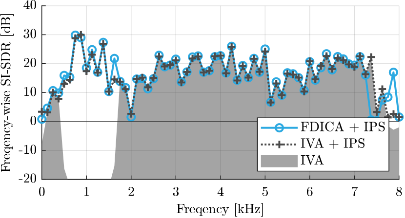
However, even when the block permutation problem arises, the demixing matrices obtained for each frequency block are often optimized correctly, except for their permutations. As an example, Fig. 3 displays the frequency-wise separation performance of the result shown in Fig. 2 (b). We calculated the frequency-wise version of the scale-invariant signal-to-distortion ratio (SI-SDR) of the separated signals in the time-frequency domain as follows:
| (6) |
where is the scaled version of the th true source signal at the th bin, i.e.,
| (7) |
and complex conjugation is denoted by . The area filled with light gray in Fig. 3 corresponds to the separation result of IVA in Fig. 2 (b). The dotted line shows IVA + IPS, where IPS ideally resolved the permutation problem of the result of IVA so that the correlation between the separated signal and the true source is maximized (see Eq. (26)). For reference, the blue line indicates FDICA with IPS (FDICA + IPS). In this example, the separation performance of IVA was extremely bad within 0.5 to 1.5 kHz, which corresponds to the middle-frequency block in Fig. 2 (b), where the red source is extracted. However, IVA + IPS was comparable to that of FDICA + IPS across all frequencies, which highlights that if the block permutation was circumvented, then IVA performs effectively. This observation motivates us to propose some specialized techniques to avoid the block permutation problem for IVA or other existing BSS algorithms.
While the block permutation problem arises from various factors, one major factor is considered to be the difficulty in handling the complicated structure of audio signals. In speech signals, for example, there are two main components: vowels dominating the lower-frequency bands and consonants appearing in the higher-frequency bands. When a BSS algorithm attempts to separate the sources, it must align the permutations of these two components, which is not straightforward since they appear in different frequency bands and at different times. At the same time, locally looking at a narrower frequency band (e.g., the mid-frequency block in Fig. 2 (b)), only a few components are dominant and have a simple structure. Therefore, it should be easy for existing BSS algorithms to resolve permutations inside such narrower bands. If we split the BSS problem into a set of several BSS problems in the narrower frequency bands, then we can focus on how to align the permutations between the multiple bands. The block permutation solvers can be used for this approach with some additional computational costs, but we can resolve the block permutation problem without an additional cost, as described in the next section.
3 Proposed Method
To solve the block permutation problem without paying additional costs, we propose a simple technique named subband splitting. The proposed method splits all the frequencies into several subbands and sequentially separates them using existing BSS methods. Narrowing the frequency band makes it easier to resolve permutations within each subband. Then, the permutations between the subbands are aligned by using the separation result in one subband as the initial values for the subsequent subbands. As in Fig. 2 (c), our method enhances the separation performance of IVA without modifying the algorithm. Here, we introduce the proposed technique and describe the way to generate the subbands used in our technique. Subsequently, we note the number of iterations and the computational cost of the proposed technique.
3.1 Subbands and BSS Method
In the proposed method, the entire frequencies are split into subbands , where the th subband is the set of frequency indices,
| (8) |
is the number of frequency bins, and and are the lower and upper bounds for the th subband , respectively. All frequency indices must be contained in at least one subband, and hence must satisfy
| (9) |
Additionally, the adjacent subbands must overlap, i.e.,
| (10) |
For notational convenience, let the separation procedure of a BSS algorithm (e.g., IVA and ILRMA) be written as
| (11) |
where the BSS algorithm receives an observed signal , an initial value of the demixing matrix , and initial values of other auxiliary variables (e.g., NMF variables and of ILRMA in Eq. (5) or any other variables necessary for the BSS algorithm). After running the BSS algorithm, it returns separated signals , the corresponding demixing matrix , and the corresponding auxiliary variables .
3.2 Proposed Method: Subband Splitting
Using the above notation, the proposed subband splitting for any BSS algorithm is given as follows:
| (12) |
where is the operator that extracts the part of variables corresponding to the th subband . The extracted part is indicated by the subscript as
| (13) |
The operator substitutes the extracted part of the variables back into their original location as
| (14) |
namely, the part of optimization variables associated with the subband are replaced with the latest optimization result provided by . The proposed method repeats Eq. (12) for so that is applied to all the subbands.
Note that and for the auxiliary variables should be defined similarly, depending on the BSS algorithms used in each subband. Specific definitions of the extraction/substitution operators for SS-IVA and SS-ILRMA are described in Section 4.1
The most important aspect of the proposed method is the existence of the overlap of the subbands. In the overlapping part , the output of within the th subband is carried over to the th subband as the initial value for . Therefore, within the th subband, the BSS algorithm is induced to obtain the same permutation as that obtained in the th subband. This initialization strategy can keep consistent permutation among the subbands if there are sufficient overlaps.
3.3 Subband Generation by Shift Rules
To generate the subbands, we define shift rules that constantly shift the subbands upward or downward:
| (15) |
where is the amount of shift.
To easily compare the settings for subbands, we introduce subband parameter . The parameter determines the width of subband and the parameter controls the amount of shift as follows:
| (16) |
where is the ceiling function. That is, the width of each subband is times the entire number of frequency bins . The subband is shifted by the amount of another times the bandwidth .
To ensure that all the frequencies, including the highest and the lowest, are updated by the same number, we set the first bounds as follows:
| (17) |
Using Eq. (17), all the frequency bins are included in subbands. Namely, for every frequency (including the lowest and the highest), BSS methods are applied by the same number, i.e., times222 This may not be true when is neither an integer nor a divisor of . For example, when , BSS methods are applied either 2 or 3 times for each frequency bin, where denotes the flooring function. . Note that the first and the last bounds overflow the entire frequency band , i.e., or holds for smaller and larger . Such bounds are clipped to the range of to when each subband is calculated (see Eq. (8)), and then the corresponding subbands become narrower than . For instance, the first subband and (when is a divisor of ) the last subband have only frequency bins.
Figure 4 illustrates an example of the subbands generated by the above rule. Here, the subband parameter is set to , i.e., the bandwidth is , and the amount of shift is . All the frequency bins are included in 2 subbands. The subband splitting with the shift rule is summarized in Alg. 1, where any BSS method can be used for .

3.4 Number of Inner Iteration and Computational Cost
Two iterations appear in the proposed method: (i) the outer iteration , where is sequentially applied to the subbands , and (ii) the inner iteration that corresponds to the iterative updates in .
Here, we confirm the relationship between the parameter , the number of inner iterations , and the total number of updates , i.e., how many times the demixing matrix is updated for each frequency 333 The total number of updates of the demixing matrix for each frequency will be the same because every frequency bin is included in the same number of subbands, as described in Section 3.3. . Since the proposed method runs BSS algorithms times duplicated for each frequency, the total number of updates increases as increases, i.e.,
| (18) |
For example, in Fig. 4, all the frequency bins are updated twice because .
With fixing the number of inner iterations , the overall computational cost becomes times larger due to the duplicated run of the BSS algorithm. This increase in computational cost can be canceled by dividing the number of inner iterations by . Namely, given a total number of updates , set the number of inner iterations as follows444 The increase in computational cost due to the duplicated runs of BSS algorithms is canceled using Eq. (19) when the cost of BSS algorithms depends linearly on the number of frequency bins. This condition is satisfied with AuxIVA[12] and ILRMA[23]. :
| (19) |
Note that the proposed method can improve memory efficiency because each subband is narrower than usual.
4 Experiment
In this section, we propose SS-IVA and SS-ILRMA by combining our subband splitting with IVA and ILRMA, respectively. We also describe a conventional subband-aware method, which we call overlapped-clique-based IVA (OC-IVA) here. We then evaluate their separation performance and computational costs using speech signals. We also evaluate the separation performance of SS-ILRMA using music signals.
4.1 Proposed Method: SS-IVA and SS-ILRMA
4.1.1 SS-IVA
4.1.2 SS-ILRMA
The proposed SS-ILRMA uses ILRMA[23] for in Alg. 1. Note that ILRMA has auxiliary variables for NMF, i.e., the basis matrices and the activation matrices . Therefore, the operation of and for must be defined, as well as , and in Eqs. (13) and (14). Here, we define the extraction operation for as follows:
| (20) |
where
| (21) |
and substitution operation to do the reverse. Namely, it extracts the part of basis matrices associated with the subband , similar to demixing matrices . At the same time, it carries over the activation matrices optimized in the th subband to the th subband as initial values. This definition is based on the following intuition that the activation roughly reflects whether the th source is active at each time, and they become similar in two adjacent subbands. Carrying over a common activation matrices provides a stronger bond between the subbands and helps avoiding block permutation problems.
4.2 Comparison Method: OC-IVA[18]
To compare our subband splitting with conventional subband-aware methods, we tested OC-IVA, which is an extension of IVA[18]. Similar to the proposed method, OC-IVA considers overlapping subbands to estimate demixing matrices. The significant difference with our SS-IVA is that OC-IVA separates all frequency bands simultaneously using an algorithm derived from the following objective function:
| (22) |
where we generate the subbands in the same way with our method. Note that the first term models the subband-wise group structure (see Eq. (4) for comparison to the original IVA). Comparison with OC-IVA helps to see whether optimizing the subbands simultaneously or sequentially yields better performance.
4.3 Experimental Settings
We evaluated BSS methods using two-channel mixtures of two sources, i.e., . The speech and music signals were obtained from SiSEC 2011[40] dataset. For speech signals (Section 4.4 and 4.5), 8 speech signals were obtained from dev1 in underdetermined speech and music mixtures task[40]. Then, all 56 possible pairs (considering their permutations) were used as source signals. Their duration was 10 s, and the sampling frequency was 16 kHz. For music signals (Section 4.6), we used 4 songs from professionally produced music recordings task[40]. For each song, two instruments (including vocals, guitars, violins, and synth) were chosen as in [23, Table 3] (the paper proposed ILRMA). They were downsampled to 16 kHz.
The observed signals were generated by convolving room impulse responses in [41] with downsampling to 16 kHz. The reverberation time was 160 ms. The pair of source directions were , , and . The spacing between the two microphones was 8 cm, and the distance between the sources and the center of the microphones was 1 m.
The demixing matrices were initialized with identity matrices. All elements of the initial value for and were drawn from the uniform distribution , where five different seeds were used.
The window length and the hop size of STFT were set to 2048 and 1024 samples, respectively. The Hann window was used for the window function. The Nyquist frequency was omitted from the optimization target, i.e., the number of frequency bins was .
The source-to-distortion ratio improvement (SDRi) [43] was used to evaluate separation performance. In addition, we define permutation consistency, a weighted accuracy of permutation, as follows:
| (23) | ||||
where is the frequency-wise weight given by the power of each frequency, i.e.,
| (24) |
is Kronecker’s delta,
| (25) |
is the index of correct permutation that achieves the highest correlation between the source and separated signal at each frequency, i.e.,
| (26) |
where , is the th permutation (i.e., ), and is the set of all permutations of elements. Permutation consistency takes the values between and , and the higher, the better. The experiments were performed with MATLAB R2024b on AMD Ryzen 9 5950X (3.40 GHz, 16 core).
| Method (: ours) | SDRi [dB] | Permutation consistency [%] | |||||||||||||
|---|---|---|---|---|---|---|---|---|---|---|---|---|---|---|---|
| — | — | ||||||||||||||
| IVA | Vanilla | [12] | — | 6.11 | — | — | — | — | 85.42 | — | — | — | — | ||
| OC | [18] | — | — | 10.05 | 9.13 | 6.94 | 9.76 | — | 96.16 | 92.97 | 88.3 | 94.69 | |||
| SS | — | — | 10.09 | 10.34 | 10.82 | 10.90 | — | 96.25 | 96.81 | 97.55 | 97.77 | ||||
| SS | — | — | 10.73 | 11.00 | 10.96 | 10.53 | — | 97.29 | 97.65 | 97.60 | 95.98 | ||||
| ILRMA | Vanilla | [23] | 2 | 8.90 | — | — | — | — | 91.71 | — | — | — | — | ||
| Vanilla | [23] | 10 | 8.56 | — | — | — | — | 89.91 | — | — | — | — | |||
| SS | 2 | — | 10.01 | 11.29 | 11.50 | 10.82 | — | 94.79 | 97.75 | 98.09 | 96.46 | ||||
| SS | 10 | — | 8.91 | 11.06 | 11.03 | 9.84 | — | 92.02 | 96.90 | 96.93 | 93.97 | ||||
| SS | 2 | — | 11.25 | 11.67 | 12.06 | 11.95 | — | 97.91 | 98.78 | 99.60 | 99.49 | ||||
| SS | 10 | — | 10.57 | 10.97 | 11.71 | 11.79 | — | 96.15 | 97.21 | 98.86 | 99.12 | ||||
| FDICA + IPS | — | 12.20 | — | — | — | — | 100.00 | — | — | — | — | ||||
4.4 Separation Performance for Speech Signals
We evaluated the separation performance of BSS methods using speech signals. The total number of updates was fixed to 100. The parameters and were set to 2 or 4 to ensure that is a divisor of 100 (= ) and that is a divisor of 1024 (= ). The number of bases for ILRMA was set to 2 and 10. We also tested FDICA + IPS, the oracle method that individually separates each frequency via FDICA and solves the permutation via IPS, where IPS finds the ideal permutation using Eq. (26).
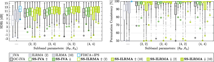
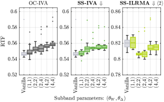
Figure 5 and Table 1 summarize their separation performance, where Vanilla refers to the original IVA or ILRMA handling all frequencies simultaneously. The experimental results show the notable improvements brought by the proposed subband splitting.
Both the conventional OC-IVA and our proposed SS-IVA outperformed Vanilla IVA, confirming that band splitting enhances separation performance. In all the settings, our SS-IVA (sequential separation) consistently outperformed OC-IVA (simultaneous separation). Notably, the permutation consistency of SS-IVA was significantly high compared to OC-IVA, which demonstrates that the sequential procedure contributes to aligning permutation.
For ILRMA, the proposed SS-ILRMA obtained the highest performance for almost all subband parameters. Downward SS-ILRMA with achieved the best result in the experiment. Remarkably, its separation performance was comparable to FDICA + IPS, and the permutation consistency was almost perfect (99.60 on average). Moreover, even under the worst case (indicated by a large marker), it resulted in dB in SDRi, which was dB higher than Vanilla ILRMA ( dB). Note that the average performance of ILRMA and SS-ILRMA tended to be better when rather than when . At the same time, when , the downward SS-ILRMA with achieved similar performance as (see Fig. 5), indicating that splitting into smaller subbands reduces the size of the problem within each subband and helps the algorithms to work stably.
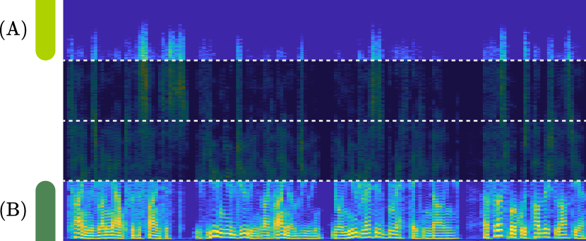
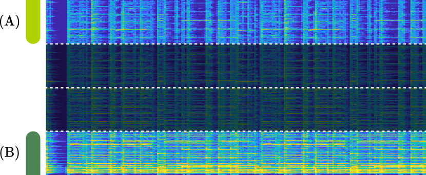
The downward shift tended to be superior to the upward shift, which was particularly noticeable in SS-ILRMA. That is, starting with the separation of higher frequency bands was more effective. This is likely due to the sparsity (an important cue for many BSS algorithms) of the speech signals in higher frequency bands. To illustrate this, Fig. 6 shows a speech signal used in the experiment along with the (A) highest and (B) lowest subbands, where the subband parameter was set to . When using the upward shift, the lowest band (B) must be separated first. However, this subband is relatively dense, making it difficult for sparsity-based BSS methods. Failures at this subband negatively affect the separation of subsequent subbands. On the other hand, when the downward shift is used, the highest subband (A) is separated first. Owing to its sparsity and simple structure (i.e., components concentrated in specific time frames and appearing as vertical patterns), this subband can be successfully separated using IVA and ILRMA. The results from the higher subbands are then propagated to the lower (i.e., more challenging) subbands and help their separation, leading to better outcomes.
4.5 Computational Costs
(a) Per number of updates.
 (b) Per RTF.
Next, we investigate the computational costs of the proposed technique using the same mixtures as in Section 4.4 We run each BSS method 20 times to measure the real-time factor (RTF), i.e., the normalized runtime required to process one second of the signal. To check the implementations, we also tested SS-IVA and SS-ILRMA with , which agrees with the Vanilla version of IVA and ILRMA. The total number of updates was fixed to 100. The downward shift was used, and the number of bases was set to since SS-IVA and SS-ILRMA were found to perform better with this setting (see Section 4.4).
The results are shown in Fig. 7. The conventional OC-IVA and the proposed SS-IVA took slightly longer runtime than Vanilla IVA due to band splitting. Their RTF increased as the subband parameters and grew. For ILRMA, the subband splitting was found to reduce the computation time. It was also observed that the runtime in SS-ILRMA was primarily influenced by , which determines the bandwidth , and was less dependent on , which controls the amount of shift .
We also examined the relationship between computational time and separation performance. The total number of updates was varied from 0 to 100 in increments of 4. For each method, the best subband parameters in Table 1 were used: for OC-IVA, for downward SS-IVA, and for downward SS-ILRMA with .
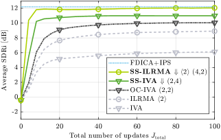
Figure 8 (a) shows the average separation performance against the total number of updates . The separation performance of conventional IVA and ILRMA grew gradually, which is due to some mixtures that require many iterations for resolving the permutation problem. On the other hand, the proposed SS-IVA and SS-ILRMA rapidly converged in fewer iterations. SS-IVA reached the ceiling of the separation performance around , and SS-ILRMA around . The required number of updates (i.e., 12 and 8) is less than half compared to that in the previous literature, e.g., [23], thanks to the ability to avoid erroneous permutation.
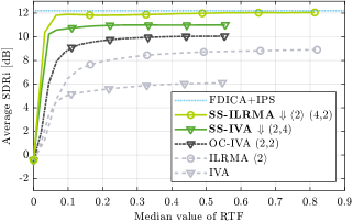
Figure 8 (b) shows the average separation performance versus RTF. The proposed SS-IVA and SS-ILRMA were confirmed to converge with shorter runtimes than conventional methods.
4.6 Separation Performance for Music Signals
From the experimental results so far, we have confirmed that, for speech signals, SS-ILRMA is highly effective. This might be a surprising outcome because ILRMA is known to be unsuitable for speech signals but suitable for music signals. Therefore, we additionally evaluated SS-ILRMA on music signals. The parameters are the same as in Section 4.4
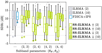
Figure 9 and Table 2 show the separation performance of ILRMA, SS-ILRMA, and FDICA+IPS. When the number of basis was set to 10, the Vanilla ILRMA performed worse in some cases555 When only evaluating the song ID4 in [23, Table 3] (i.e., guitar and synth in [23, Fig. 12] that investigates the relationship between and SDRi), the average SDRi of Vanilla ILRMA was 16.24 dB () and 16.62 dB (), i.e., outperformed , which agrees with [23, Fig. 12]. The poor performance of Vanilla ILRMA with in Fig. 9 is due to the other mixtures, especially ID2 and ID3. . The upward SS-ILRMA was ineffective for music signals, while the downward SS-ILRMA performed robustly for both and . In particular, the downward SS-ILRMA with yielded the best results in terms of the median SDRi, where the worst-case SDRi was improved by 7.51 dB compared to Vanilla ILRMA with . Note that downward SS-ILRMA with , , and even outperformed FDICA+IPS on average, which might be because SS-ILRMA can more precisely model the structure of the power spectrogram (including the relationship among the time-frequency bins) by using NMF, while FDICA handles the frequency bins independently.
| Method | SDRi [dB] | |||||||
|---|---|---|---|---|---|---|---|---|
| (: ours) | — | |||||||
| Vanilla | [23] | 2 | 11.65 | — | — | — | — | |
| Vanilla | [23] | 10 | 9.99 | — | — | — | — | |
| SS | 2 | — | 9.75 | 7.02 | 6.96 | 6.97 | ||
| SS | 10 | — | 9.75 | 4.67 | 4.66 | 5.75 | ||
| SS | 2 | — | 11.89 | 11.48 | 12.32 | 11.59 | ||
| SS | 10 | — | 12.29 | 11.53 | 11.61 | 10.85 | ||
| FDICA+IPS | — | 11.71 | — | — | — | — | ||
The difference between upward and downward shifts was more pronounced in music signals compared to that in speech signals (Section 4.4). This should be because the separation of lower frequency bands in music signals can be significantly challenging for some instruments. As an example, Fig. 10 shows the signal of the guitar used in the experiment. Similar to speech signals, the highest subband (A) is sparse. On the contrary, the lowest subband (B) is even denser than that of speech signals. Therefore, the downward shift, i.e., leveraging the separation result obtained from higher subbands to assist in the separation of lower subbands, is indispensable when using SS-ILRMA for music signals.
5 Conclusion
In this paper, we proposed subband splitting, a technique for improving the performance of existing BSS algorithms. It sequentially applies a BSS algorithm to several overlapping subbands. Despite its simplicity, the proposed method effectively improves the separation performance. Additionally, we proposed SS-IVA and SS-ILRMA by incorporating IVA and ILRMA into our technique. Experimental results showed that our downward SS-ILRMA reached significantly higher separation performance with rapid convergence. Future work includes integrating more advanced BSS methods (e.g., those utilizing deep learning) for further improvement of separation performance. It is also valuable to extend the proposed technique to real-time processing scenarios by leveraging its fast convergence.
References
- [1] P. Smaragdis, “Blind separation of convolved mixtures in the frequency domain,” Neurocomputing, 22(1), 21–34 (1998).
- [2] N. Murata, S. Ikeda and A. Ziehe, “An approach to blind source separation based on temporal structure of speech signals,” Neurocomputing, 41(1), 1–24 (2001).
- [3] H. Sawada, R. Mukai, S. Araki and S. Makino, “A robust and precise method for solving the permutation problem of frequency-domain blind source separation,” IEEE Trans. Speech Audio Process., 12(5), 530–538 (2004).
- [4] L. Wang, H. Ding and F. Yin, “A region-growing permutation alignment approach in frequency-domain blind source separation of speech mixtures,” IEEE Trans. Audio Speech Lang. Process., 19(3), 549–557 (2011).
- [5] A. Sarmiento, I. Durán-DÃaz, A. Cichocki and S. Cruces, “A contrast function based on generalized divergences for solving the permutation problem in convolved speech mixtures,” IEEE/ACM Trans. Audio Speech Lang. Process., 23(11), 1713–1726 (2015).
- [6] S. Yamaji and D. Kitamura, “DNN-based permutation solver for frequency-domain independent component analysis in two-source mixture case,” Asia-Pac. Signal Inf. Process. Assoc. Annu. Summit Conf. (APSIPA ASC), pp. 781–787 (2020).
- [7] F. Hasuike, D. Kitamura and R. Watanabe, “DNN-based frequency-domain permutation solver for multichannel audio source separation,” Asia-Pac. Signal Inf. Process. Assoc. Annu. Summit Conf. (APSIPA ASC), pp. 871–876 (2022).
- [8] L. Li, H. Kameoka and S. Seki, “HBP: An efficient block permutation solver using Hungarian algorithm and spectrogram inpainting for multichannel audio source separation,” IEEE Int. Conf. Acoust. Speech Signal Process. (ICASSP), pp. 516–520, IEEE (2022).
- [9] S. Emura, “Permutation-alignment method using manifold optimization for frequency-domain blind source separation,” IEEE Int. Conf. Acoust. Speech Signal Process. (ICASSP), pp. 601–605 (2024).
- [10] A. Hiroe, “Solution of permutation problem in frequency domain ICA, using multivariate probability density functions,” Independent Component Analysis and Blind Signal Separation, pp. 601–608 (2006).
- [11] T. Kim, I. Lee and T.-W. Lee, “Independent vector analysis: Definition and algorithms,” Fortieth Asilomar Conf. Signals Syst. Comput., pp. 1393–1396 (2006).
- [12] N. Ono, “Stable and fast update rules for independent vector analysis based on auxiliary function technique,” IEEE Workshop Appl. Signal Process. Audio Acoust. (WASPAA), pp. 189–192 (2011).
- [13] R. Scheibler and N. Ono, “Fast and stable blind source separation with rank-1 updates,” IEEE Int. Conf. Acoust. Speech Signal Process. (ICASSP), pp. 236–240 (2020).
- [14] K. Yatabe and D. Kitamura, “Time-frequency-masking-based determined BSS with application to sparse IVA,” IEEE Int. Conf. Acoust. Speech Signal Process. (ICASSP), pp. 715–719 (2019).
- [15] K. Yatabe and D. Kitamura, “Determined BSS based on time-frequency masking and its application to harmonic vector analysis,” IEEE/ACM Trans. Audio Speech Lang. Process., 29, 1609–1625 (2021).
- [16] Y. Liang, S. M. Naqvi and J. Chambers, “Overcoming block permutation problem in frequency domain blind source separation when using AuxIVA algorithm,” Electron. Lett., 48(8), 460 – 462 (2012).
- [17] G.-J. Jang, I. Lee and T.-W. Lee, “Independent vector analysis using non-spherical joint densities for the separation of speech signals,” IEEE Int. Conf. Acoust. Speech Signal Process., Vol. 2, pp. II–629–II–632 (2007).
- [18] I. Lee and G.-J. Jang, “Independent vector analysis based on overlapped cliques of variable width for frequency-domain blind signal separation,” EURASIP J. Adv. Signal Process., 2012(1), 113 (2012).
- [19] R. Ikeshita, Y. Kawaguchi, M. Togami, Y. Fujita and K. Nagamatsu, “Independent vector analysis with frequency range division and prior switching,” Eur. Signal Process. Conf. (EUSIPCO), pp. 2329–2333 (2017).
- [20] U.-H. Shin and H.-M. Park, “Auxiliary-function-based independent vector analysis using generalized inter-clique dependence source models with clique variance estimation,” IEEE Access, 8, 68103–68113 (2020).
- [21] L. Li and K. Koishida, “Geometrically constrained independent vector analysis for directional speech enhancement,” IEEE Int. Conf. Acoust. Speech Signal Process. (ICASSP), pp. 846–850 (2020).
- [22] K. Goto, T. Ueda, L. Li, T. Yamada and S. Makino, “Geometrically constrained independent vector analysis with auxiliary function approach and iterative source steering,” Eur. Signal Process. Conf. (EUSIPCO), pp. 757–761 (2022).
- [23] D. Kitamura, N. Ono, H. Sawada, H. Kameoka and H. Saruwatari, “Determined blind source separation unifying independent vector analysis and nonnegative matrix factorization,” IEEE/ACM Trans. Audio Speech Lang. Process., 24(9), 1626–1641 (2016).
- [24] H. Sawada, N. Ono, H. Kameoka, D. Kitamura and H. Saruwatari, “A review of blind source separation methods: Two converging routes to ILRMA originating from ICA and NMF,” APSIPA Trans. Signal Inf. Process., 8(1), (2019).
- [25] D. Kitamura and K. Yatabe, “Consistent independent low-rank matrix analysis for determined blind source separation,” EURASIP J. Adv. Signal Process., 2020(1), 46 (2020).
- [26] S. Mogami, D. Kitamura, Y. Mitsui, N. Takamune, H. Saruwatari and N. Ono, “Independent low-rank matrix analysis based on complex Student’s t-distribution for blind audio source separation,” IEEE Int. Workshop Mach. Learn. Signal Process. (MLSP), pp. 1–6 (2017).
- [27] S. Mogami, Y. Mitsui, N. Takamune, D. Kitamura, H. Saruwatari, Y. Takahashi, K. Kondo, H. Nakajima and H. Kameoka, “Independent low-rank matrix analysis based on generalized Kullback-Leibler divergence,” IEICE Trans. Fundam. Electron. Commun. Comput. Sci., E102.A(2), 458–463 (2019).
- [28] Y. Mitsui, N. Takamune, D. Kitamura, H. Saruwatari, Y. Takahashi and K. Kondo, “Vectorwise coordinate descent algorithm for spatially regularized independent low-rank matrix analysis,” IEEE Int. Conf. Acoust. Speech Signal Process. (ICASSP), pp. 746–750 (2018).
- [29] F. Oshima, M. Nakano and D. Kitamura, “Interactive speech source separation based on independent low-rank matrix analysis,” Acoust. Sci. Technol., 42(4), 222–225 (2021).
- [30] R. Ikeshita and Y. Kawaguchi, “Independent low-rank matrix analysis based on multivariate complex exponential power distribution,” IEEE Int. Conf. Acoust. Speech Signal Process. (ICASSP), pp. 741–745 (2018).
- [31] N. Makishima, S. Mogami, N. Takamune, D. Kitamura, H. Sumino, S. Takamichi, H. Saruwatari and N. Ono, “Independent deeply learned matrix analysis for determined audio source separation,” IEEE/ACM Trans. Audio Speech Lang. Process., 27(10), 1601–1615 (2019).
- [32] T. Hasumi, T. Nakamura, N. Takamune, H. Saruwatari, D. Kitamura, Y. Takahashi and K. Kondo, “Empirical Bayesian independent deeply learned matrix analysis for multichannel audio source separation,” Eur. Signal Process. Conf. (EUSIPCO), pp. 331–335 (2021).
- [33] T. Hasumi, T. Nakamura, N. Takamune, H. Saruwatari, D. Kitamura, Y. Takahashi and K. Kondo, “PoP-IDLMA: Product-of-prior independent deeply learned matrix analysis for multichannel music source separation,” IEEE/ACM Trans. Audio Speech Lang. Process., 31, 2680–2694 (2023).
- [34] H. Kameoka, L. Li, S. Inoue and S. Makino, “Supervised determined source separation with multichannel variational autoencoder,” Neural Comput., 31(9), 1891–1914 (2019).
- [35] L. Li, H. Kameoka and S. Makino, “Fast MVAE: Joint separation and classification of mixed sources based on multichannel variational autoencoder with auxiliary classifier,” IEEE Int. Conf. Acoust. Speech Signal Process. (ICASSP), pp. 546–550 (2019).
- [36] L. Li, H. Kameoka and S. Makino, “FastMVAE2: On improving and accelerating the fast variational autoencoder-based source separation algorithm for determined mixtures,” IEEE/ACM Trans. Audio, Speech and Lang. Proc., 31, 96â110 (2022).
- [37] R. Scheibler and M. Togami, “Surrogate source model learning for determined source separation,” IEEE Int. Conf. Acoust. Speech Signal Process. (ICASSP), pp. 176–180 (2021).
- [38] K. Matsumoto and K. Yatabe, “Determined BSS by combination of IVA and DNN via proximal average,” IEEE Int. Conf. Acoust. Speech Signal Process. (ICASSP), pp. 871–875 (2024).
- [39] K. Matsumoto and K. Yatabe, “Subband splitting: Simple, efficient and effective technique for solving block permutation problem in determined blind source separation,” arXiv:2409.09294 (2024).
- [40] S. Araki, F. Nesta, E. Vincent, Z. Koldovský, G. Nolte, A. Ziehe and A. Benichoux, “The 2011 signal separation evaluation campaign (SiSEC2011): - audio source separation -,” Latent Var. Anal. Signal Sep., pp. 414–422 (2012).
- [41] E. Hadad, F. Heese, P. Vary and S. Gannot, “Multichannel audio database in various acoustic environments,” Int. Workshop Acoust. Signal Enhanc. (IWAENC), pp. 313–317 (2014).
- [42] C. Févotte, N. Bertin and J.-L. Durrieu, “Nonnegative matrix factorization with the Itakura-Saito divergence: With application to music analysis,” Neural Comput., 21(3), 793–830 (2009).
- [43] E. Vincent, R. Gribonval and C. Fevotte, “Performance measurement in blind audio source separation,” IEEE Trans. Audio Speech Lang. Process., 14(4), 1462–1469 (2006).
Kazuki Matsumotois currently an undergraduate student at Waseda University. His research interests include optimization-based signal processing.
Kohei Yatabereceived the B.E., M.E., and Ph.D. degrees from Waseda University in 2012, 2014, and 2017, respectively. He is currently an Associate Professor at the Department of Electrical Engineering and Computer Science at the Tokyo University of Agriculture and Technology.