Subharmonic Dynamics of Wave Trains in the Korteweg-de Vries / Kuramoto-Sivashinsky Equation
Abstract
We study the stability and nonlinear local dynamics of spectrally stable periodic wave trains of the Korteweg-de Vries / Kuramoto-Sivashinsky equation when subjected to classes of periodic perturbations. It is known that for each , such a -periodic wave train is asymptotically stable to -periodic, i.e., subharmonic, perturbations, in the sense that initially nearby data will converge asymptotically to a small Galilean boost of the underlying wave, with exponential rates of decay. However, both the allowable size of initial perturbations and the exponential rates of decay depend on and, in fact, tend to zero as , leading to a lack of uniformity in such subharmonic stability results. Our goal here is to build upon a recent methodology introduced by the authors in the reaction-diffusion setting and achieve a subharmonic stability result which is uniform in . This work is motivated by the dynamics of such wave trains when subjected to perturbations which are localized (i.e., integrable on the line).
1 Introduction
In this work, we consider the local dynamics of wave trains, i.e., periodic traveling wave solutions, of the Korteweg-de Vries / Kuramoto-Sivashinsky (KdV/KS) equation
| (1.1) |
where . Here, and are modeling parameters which may, without loss of generality, be chosen such that : see Remark 1.1 below. The equation (1.1) is known to be a canonical model for pattern formation that has been used to describe many applications including plasma instabilities, turbulence in reaction diffusion equations, flame front propagation, and nonlinear wave dynamics in fluid mechanics [20, 21, 7, 15, 16]. In the case and , equation (1.1) becomes the classical Kuramoto-Sivashinsky equation, which is known to be a generic equation for chaotic dynamics, and there is a very large literature on these solutions, their bifurcations and period doubling cascades, and their stability: see, for example, [9] and reference therein. In this case, (1.1) is also known to model thin film dynamics down a completely vertical wall [6]. When the angle of the wall is decreased from vertical, however, additional dispersive effects are present [9] and modeled by , and in the “flat” limit where the inclined wall becomes horizontal one recovers the completely integrable Korteweg-de Vries equation, corresponding here to and . Thus, in the context of inclined thin film flow one can consider the general model (1.1) as interpolating between the vertical wall and the “flat” limit . For more information on the connection to thin film dynamics, as well as its derivation in this context from the viscous shallow water equations or the full Navier Stokes equations, see [24, 25].
Remark 1.1.
In the literature, one may encounter more general looking systems of the form
where here and are arbitrary constants. However, we note that, through a rescaling argument, such systems can always be put in the form (1.1), i.e., one can always take and with . See [3, Section 2]. Note the particular scaling here is sometimes referred to as the “thin film” scaling: see [9] for example.
In this work, we are interested in understanding the stability and long-time dynamics of periodic traveling wave solutions of (1.1) to specific classes of perturbations. To begin our discussion, we briefly discuss the existence theory for periodic solutions of (1.1). First, note that traveling wave solutions of (1.1) correspond to solutions of the form , where necessarily satisfies the profile ODE
| (1.2) |
The existence and local structure of periodic solutions of (1.2) has been studied extensively by several other authors. For general values of , an elementary Hopf bifurcation analysis [3] shows the existence of a -parameter family of asymptotically small amplitude periodic traveling wave solutions of (1.2) which, up to translation, can be parametrized by the wave speed and the period . In the “classical KS” limit , one can likewise use normal form analysis to establish a similar existence result [9], while the full bifurcation picture for the KS equation () is known to be extremely complicated: see, for example, [14], where the authors prove the existence of a Shi’lnikov bifurcation which leads to cascades of period doubling, period multiplying -bifurcations and oscillatory homoclinic orbits as the period is increased, as well as the numerical bifurcation study in [4]. For a summary and more details, see [3, 11].
Using the above existence studies as motivation, and closely following the work in [3], we make the following assumption regarding the existence of periodic solutions of (1.2), as well as the structure of the local manifold of periodic solutions.
Assumption 1.2.
Remark 1.3.
It is natural to assume (1.2) admits a -dimensional manifold of periodic solutions. Indeed, note that integrating the profile equation (1.2) once yields
for some constant of integration . Periodic solutions of (1.2) thus correspond to values
where , , and denote the period, wave speed and constant of integration, subjected to the periodicity condition
leading, generically, to a -parameter family of periodic solutions parametrized, up to translation, by the period , the wave speed .
As stated above, our main goal is to study the stability and dynamics of periodic traveling wave solutions of (1.1) to specific classes of perturbations. Previously, there has been much work regarding both the spectral and nonlinear stability of such periodic solutions when subjected to localized perturbations, i.e., perturbations that are integrable on the line [3, 2, 11], as well as their dynamics under slow-modulations [17]. In these works, it is found that for each admissible pair in (1.1) there exist periodic traveling wave solutions which are spectrally and nonlinearly stable to localized perturbations. Here, however, we study the stability and dynamics of -periodic traveling wave solutions of (1.1) when subject to so-called subharmonic perturbations, i.e., -periodic perturbations for some . Before we continue, we note that an extremely important feature of (1.1), which we utilize heavily in our forthcoming analysis, is the presence of a Galilean symmetry. In particular, if is a solution of (1.1), then so is the function
| (1.3) |
for any . Thanks to this Galilean invariance, as well as the translational invariance of (1.1), it follows that the stability of a particular wave only depends on one parameter: namely, the period . Thus, when discussing the stability of periodic traveling wave solutions of the KdV-KS equation (1.1), we identify all waves of a particular period. Furthermore, note we can view (1.3) as coupling between the wave speed and the mass of the wave, defined via
which is readily seen to be a conserved quantity of (1.1) due to the conservative structure.
Now, suppose that is a -periodic solution of (1.2) with wave speed , and note the linearization of (1.1) (in the appropriate co-moving frame) about is given by the operator
Since we are considering subharmonic perturbations of , i.e., perturbations with period for some , here we consider as a closed, densely defined linear operator acting on with -periodic coefficients. To describe the spectrum of acting on , first observe that one always has that
| (1.4) |
so that is an eigenvalue of with algebraic multiplicity at least two and a Jordan chain of height at least one. With this in mind, and following the works [19, 18, 10, 13], we introduce the notion of spectral stability used throughout this work.
Definition 1.4.
A -periodic traveling wave solution of (1.2) is said to be diffusively spectrally stable provided the following conditions hold:
-
(D1)
The spectrum of the linear operator acting on satisfies
-
(D2)
There exists a such that for any the real part of the spectrum of the Bloch operator acting on satisfies
-
(D3)
is a -periodic eigenvalue of with algebraic multiplicity two and geometric multiplicity one.
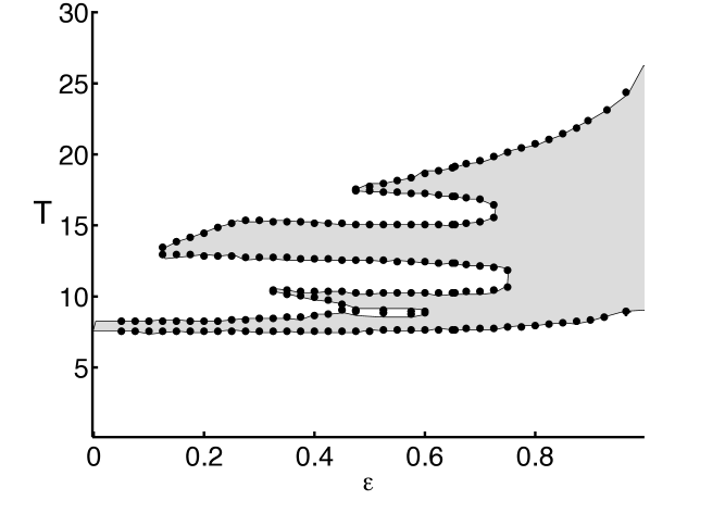
We note that in [3] it was shown that for every admissible pair of modeling parameters there exists a range of periods for which all periodic traveling wave solutions of (1.1) with those period are diffusively spectrally stable: see Figure 1 and also [1, 5]. In the context of the KdV/KS equation (1.1), it is known that diffusively spectrally stable periodic traveling wave solutions (coupled with an additional non-degeneracy hypothesis, see Assumption 1.5 below) are nonlinearly stable to localized perturbations, in the sense that localized perturbations of such a periodic waves converges to spatially localized phase modulations of . Specifically, given such a periodic traveling wave and initial data
then for large time the associated solution satisfies
for some function which behaves essentially like a finite sum of (small) error functions: see [3]. As we will see below, the implication of diffusive spectral stability will be that such a -periodic traveling wave is necessarily spectrally stable to perturbations in for every .
Before continuing to state our main result, we introduce an additional non-degeneracy hypothesis. As we will see in Lemma 2.1 below, Assumption 1.2, along with the diffusive spectral stability assumption, implies that for small the Bloch operators have two eigenvalues near the origin which expand as
| (1.5) |
for . Following the previous work [3, 10], we make the following additional non-degeneracy hypothesis:
Assumption 1.5.
The coefficients in (1.5) are distinct.
By standard spectral perturbation theory, Assumption 1.5 ensures the analyticity of the functions in (1.5): again, see Lemma 2.1 below. Furthermore, it is known that the coefficients are the characteristics of an associated Whitham averaged system, formally governing slowly modulated periodic solutions of (1.1). Consequently, Assumption 1.5 corresponds to strict hyperbolicity of the Whitham averaged system. See [17] for more details. Note also that all the diffusively spectrally stable periodic traveling wave solutions in Figure 1 were seen numerically to satisfy Assumption 1.5.
We now begin our discussion of our main results concerning the dynamics of -periodic, diffusively spectrally stable traveling wave solutions of (1.1) when subjected to subharmonic perturbations. First, in Section 2.1 we will see that the spectrum of acting on is given by the union of the (necessarily discrete) spectrum of the corresponding Bloch operators acting in for the discrete (finite) subset of such that . Thus, such a traveling wave is necessarily spectrally stable to all subharmonic perturbations. In particular, for each there exists a constant such that
Since is clearly sectorial, it is easy to show that for fixed and there exists a constant such that
| (1.6) |
for all , where here denotes the projection of onto the -periodic generalized kernel of . Equipped with this linear estimate and exploiting the Galilean invariance (1.3), the following nonlinear stability result was established in [22, 23] for the case and is easily extended to general .
Proposition 1.6 (Nonlinear Subharmonic Stability [22, 23]).
Let be a -periodic traveling wave solution of (1.1) with wave speed . Assume that is diffusively spectrally stable and additionally satisfies Assumption 1.5. Fix and take such that
holds. Then for each and for every , there exists an and a constant such that whenever and , then the solution of (1.1) with initial data exists globally in time and satisfies
for all , where here is some constant and
The above result establishes the nonlinear asymptotic stability of the Galilean family associated to , showing that nearby -periodic solutions will, up to a spatial translation, asymptotically converge to a member of the Galilean family of . However, Proposition 1.6 lacks uniformity in in two important ways. Specifically, both the exponential rate of decay and the allowable size of initial perturbations are controlled by the size of the spectral gap . Since it is known that as , it follows that both and in Proposition 1.6 must necessarily tend to zero as . Of course, from a practical level it would be preferable to develop a theory which, for a given background wave , yielded a fixed size for the theoretically prescribed domain of attraction as well as a uniform (in ) rate of decay of initial perturbations. The fact that this is possible is precisely our main result.
Theorem 1.7 (Uniform Subharmonic Asymptotic Stability).
Let be a -periodic traveling wave solution of (1.1) with wave speed . Assume that is diffusively spectrally stable and, additionally, satisfies Assumption 1.5. There exists an and a constant such that, for every , whenever and
there exists a function satisfying such that the solution of (1.1) with initial data exists globally in time and satisfies
| (1.7) |
for all .
The main difficulty in establishing the proof of Theorem 1.7 appears at the linear level. Specifically, one must develop a strategy to handle the accumulation of -periodic eigenvalues near for in a uniform way. In the proof of Proposition 1.6, this accumulation is handled by enclosing the origin in the spectral plane in an small ball where the -dependent radius is chosen so that
| (1.8) |
and defining the associate Riesz spectral projection
| (1.9) |
onto the -periodic generalized kernel of . One then decomposes the linear solution operator (semigroup) as
and uses the exponential bound (1.6) to establish the result. The lack of uniformity in Proposition 1.6, however, stems from the fact that the radius of the ball used in the Riesz projection (1.9) must necessarily tend to zero as in order to maintain the spectral decomposition (1.8).
To establish the uniformity in Theorem 1.7, however, we cannot allow the radius of the ball about the origin to shrink. Instead, we define a ball with an -independent radius and define the associated Riesz spectral projection associated to the total generalized eigenspace corresponding to eigenvalues interior to the ball. Naturally, the dimension of this total eigenspace is tending to infinity as , and we must work to establish uniform in decay estimates associated with the induced decomposition of the semigroup. This methodology was first introduced, at the linear level, by the authors and collaborators in [8] and was further extended, in the context of reaction-diffusion systems, to the full nonlinear level in [12], and is closely modeled off of the known stability theory for localized perturbations [10]. In the present work, the additional complication (compared to these previous subharmonic works) is the presence of a non-trivial Jordan block (1.4) which, in turn, yields slower uniform decay rates of the associated linear semigroups as compared to those rates in the reaction-diffusion context.
Finally, we make a few remarks concerning the connection between Proposition 1.6 and Theorem 1.7. The analysis in Section 4 shows that the modulation function in Theorem 1.7 can be decomposed as
where here satisfies
| (1.10) |
for some constant independent of . Further, while our methods fail to directly yield convergence111This is due to the presence of a non-trivial Jordan block associated with the co-periodic Bloch opertaor , leading to slower linear decay rates in Section 3 when compared to, for example, the reaction-diffusion context where no such Jordan block is present (see [12] for details). of as , one immediate observation is that for each fixed and -periodic solution of (1.1) with initial data sufficiently close (in ) to , then using the notation from both Proposition 1.6 and Theorem 1.7 we have
for some (-dependent) constant . This leads one to expect that, under relatively generic circumstances, for each fixed one should have
as . Understanding this convergence rigorously is an interesting remaining problem from our analysis.
The outline of this paper is as follows. In Section 2 we briefly review the application of Floquet-Bloch theory to subharmonic perturbations and collect several properties of the Bloch operators and their associated semigroups. We further establish basic “high-frequency” decay properties of the Bloch semigroups that arise as consequences of the diffusive spectral stability assumption. In Section 3 we provide a delicate decomposition of the semigroup acting on which will yield polynomial decay rates on the semigroup which are uniform in : see Proposition 3.1. This linear decomposition then motivates in Section 4 a nonlinear decomposition of a small neighborhood of the underlying diffusively stable -periodic background wave . Equipped with this nonlinear decomposition, along with the linear estimates from Section 3, we apply a nonlinear iteration scheme to corresponding system of perturbation equations, yielding a proof of our main result Theorem 1.7 above.
Acknowledgments: The work of MAJ was partially funded by the NSF under grant DMS-2108749, as well as the Simons Foundation Collaboration grant number 714021.
2 Preliminaries
Here, we review several preliminary analytical results. We begin with a brief review of the application of Floquet-Bloch theory to subharmonic perturbations, and then use this to establish some elementary semigroup estimates for the associated Bloch operators. For notational convenience, for each , , and fixed period we introduce the notation
and similarly with all associated Sobolev spaces.
2.1 Floquet-Bloch Theory for Subharmonic Perturbations
We begin by reviewing the results of Floquet-Bloch theory when applied to subharmonic perturbations. For more details, see the recent works [8, 12].
Suppose that is a -periodic traveling wave solution of (1.1) with wave speed , and consider the associated linearized operator . For each fixed , define222Observe that is always a finite set with and with the distance between any two closest elements being .
and note that, since the coefficients of are -periodic, basic results in Floquet-theory implies that any -periodic solution of the ordinary differential equation
must be of the form
for some and . More specifically, one can show that is an -periodic eigenvalue of if and only if there exists a such that the problem
admits a non-trivial solution in , where here the operators are known as the Bloch operators associated to and the parameter is referred to as the Bloch frequency: see also Definition 1.4. In fact, we have the spectral decomposition
which characterizes the -periodic spectrum of in terms of the union of a -periodic eigenvalues for the -parameter family of Bloch operators .
From above, it is natural when studying such -periodic spectral problems to desire to decompose arbitrary functions as superpositions of functions of the form with . To this end, given a function we define the -periodic Bloch transform of as
where now denotes the Fourier transform of on the torus given by
| (2.1) |
In particular, observe that for any and , the function is -periodic and, furthermore, the function can be recovered via the inverse Bloch representation formula
One can check that the -periodic Bloch transform
as defined above satisfies the subharmonic Parseval identify
| (2.2) |
valid for all . Finally, we note that if and then
and, additionally, we have the identity
| (2.3) |
With the above functional analytic tools in hand, we readily see that for our given linearized operator and we have
so that the operators may be viewed as operator-valued symbols under acting on . Similarly, since the operators and are clearly sectorial on their respective domains, they clearly generate analytic semigroups on and , respectively, and further their associated semigroups satisfy
| (2.4) |
In particular, we see that the -periodic Bloch transform diagonalizes the periodic coefficient operator differential acting on in the same way that the Fourier transform diagonalizes constant-coefficient differential operators acting on . This decomposition formula will be used heavily in our forthcoming linear stability estimates.
2.2 Diffusive Spectral Stability & Basic Properties of Bloch Semigroups
With the above preliminaries, we now establish some important immediate consequences of the diffusive spectral stability assumption. As a first result, we describe the unfolding of the Jordan block (1.4) for the Bloch operators for . This result for the KdV/KS system (1.1) was established in [3, Section 3.1]. See also [10] for a more general version of the same result.
Lemma 2.1 (Spectral Preparation).
Suppose that is a -periodic traveling wave solution of (1.1) which is diffusively spectrally stable and, additionally, satisfies Assumption 1.5. Then the following properties hold.
-
(i)
For any fixed there exists a constant such that
for all with .
-
(ii)
There exist positive constants and such that for all , the spectrum of decomposes into two disjoint subsets
with the following properties:
-
(a)
and .
-
(b)
The set consists of precisely two eigenvalues, which are analytic in and expand as
for and some constants (distinct) and .
-
(c)
The left and right -periodic eigenfunctions and of associated with above, normalized so that
are given as
where the functions are analytic functions such that and are dual bases of the total eigenspace of associated with the spectrum chosen to satisfy
where is a generalized left eigenfunction satisfying as well as
and where the are analytic functions.
-
(a)
Noting again that the Bloch operators are sectorial on , the spectral results in Lemma 2.1 immediately imply the following elementary estimates for the Bloch semigroups .
Proposition 2.2.
Suppose that is a -periodic traveling wave solution of (1.1) which satisfies the hypothesis of Lemma 2.1. Then the following properties hold.
-
(i)
For any fixed , there exist positive constants and such that
is valid for all and all with .
-
(ii)
With chosen as in Lemma 2.1(ii), there exist positive constants and such that for any , if denotes the (rank-two) spectral projection onto the generalized eigenspaces associated to the critical eigenvalues , then
is valid for all .
3 Subharmonic Linear Estimates
The goal of this section is to obtain decay estimates on the semigroup acting on which are uniform in . To this end, we use (2.4) to study the action of on in terms of the associated Bloch operators. Naturally, by Lemma 2.1 we expect for each fixed that the long-time behavior of is dominated by the generalized kernel of . As discussed in the introduction, the main difficulty in obtaining such a result while maintaining uniformity in is the accumulation of -periodic eigenvalues near the origin as . This is overcome through a delicate decomposition of , separating the action into appropriate critical (i.e., corresponding to spectrum accumulating near the origin) and non-critical frequency components. This methodology is heavily influenced by the corresponding decomposition used in the case of localized perturbations of periodic waves: see, for example, [10]. Note, further, that while our basic strategy is similar to the recent subharmonic analysis of reaction diffusion equations conducted in [12], the new challenge here is the fact that the linearized operator now has two spectral curves which pass through the origin, a reflection of the non-trivial Jordan structure in (1.4).
To begin, let be defined as in Lemma 2.1 and let be a smooth cutoff function satisfying for and for . Given a function , we then use (2.4) to decompose the action of on into high-frequency and low-frequency components via
| (3.1) |
Using Proposition 2.2(i), it follows that there exist constants , both independent of , such that
which, by the subharmonic Parseval identity (2.2), implies the exponential estimate
on the high-frequency component of the solution operator.
For the low-frequency component, define for each the rank-two spectral projection onto the critical modes of by
Note we also have the alternate representation formula
which more explicitly demonstrates the singularity as of the eigenprojection. Using this, the low-frequency operator can be further decomposed into the contribution from the critical modes near and the contribution from the low-frequency spectrum bounded away from via
| (3.2) |
As above, by possibly choosing smaller, Proposition 2.2(ii) implies that there exists a constant such that for each we have
for each , and hence another application of Parseval’s identity (2.2) yields
For the critical component, we decompose further as
For the non-zero frequencies, noting that Lemma 2.1 implies that the eigenfunctions of expand as
for suggests the decomposition
| (3.3) |
Additionally, note the term above can be expressed as
Observing that333Indeed, observe that and clearly the associated initial condition is satisfied.
and noting that (2.3) implies the identities
we find the representation
Observe that the above representation of the contribution of the solution operator clearly demonstrates the expected linear instability444This is naturally expected due to the Jordan block at the eigenvalue of . of the underlying wave . In the forthcoming analysis nonlinear analysis, this linear instability will be compensated by allowing for Galilean boosts of the underlying wave.
Taken together, it follows that the linear solution operator acting on can be decomposed as
| (3.4) |
where here
and the operators and are defined in (3.1) and (3.2), respectively, and and are defined in (3.3). With this decomposition in hand, we now establish temporal estimates on the above which are uniform in .
Proposition 3.1 (Linear Estimates).
Suppose that is a -periodic diffusively spectrally stable traveling wave solution of (1.1) with wave speed . Given any there exists a constant such that for all , and all we have
| (3.5) |
and
| (3.6) |
Further, there exist constants such that for all , and all we have
| (3.7) |
and
| (3.8) |
Finally, there exists a constant , independent of , such that for all we have
| (3.9) |
Proof.
We begin by establishing the estimates above. To this end, first note that the definition of implies that
Since by (2.1), an application of Cauchy-Schwarz implies the existence of a constant , independent of , such that
valid for all . Using the subharmonic Parseval identity (2.2), along with Lemma 2.1, we find that
| (3.10) | ||||
where here are constants which are independent of . By Similar considerations, we find
| (3.11) |
where, again, the constants are independent of .
Continuing, note that integration by parts yields the identity
It follows that for each and integer we have
| (3.12) | ||||
where the last equality follows by integrating by parts in the term. Since Lemma 2.1 implies that is a constant vector for each , we have
which is clearly by the analytic dependence of on . Taken together, it follows that for each we have
| (3.13) |
and, similarly,
| (3.14) |
To complete the proof of the bounds, it remains to provide bounds on the discrete, -dependent sums in (3.10)-(3.14). These uniform bounds come by directly applying Lemma A.1 in [12], which states that for any integer , there exists a constant , independent of , such that555As motivation, observe that the sum can be considered as a Riemann sum approximation for the integral , which exhibits the stated temporal decay via a routine scaling argument.
Applying this result to (3.10)-(3.14) with the appropriate values of establishes the estimates stated in (3.5)-(3.8).
It remains to establish the estimates stated in (3.9). To this end, note that by similar estimates as above, the difference between and the function
| (3.15) |
is controlled by , where here for each . Further, since for each the function is actually a constant equal to , we note that
and hence, since (3.15) is in the form of a Fourier series itself, for each the function can be recognized as the convolution of with
| (3.16) |
Recognizing the above sums as -periodic Fourier series representations for Error functions, which are clearly bounded in , this establishes the first bound in (3.9). The second bound in (3.9) now follows by using precisely the same procedure as above, while noting that (3.12) implies the extra derivative on yields an extra factor in the sum (3.16) which, in turn, yields the additional decay. ∎
Before continuing to our nonlinear analysis, we first provide an interpretation of the above decomposition of the linear solution operator. To this end, suppose is a -periodic diffusively spectrally stable periodic traveling wave solution of (1.1), and suppose that is a solution (in same co-moving frame) with initial data with and . From the decomposition (3.4) and the linear estimates in Proposition 3.1, it is then natural to suspect that
which is a (small, via the bounds in (3.9)) spatio-temporal phase modulation of the background wave together with an (identical) wave-speed and mass correction. In particular, recalling that solutions of the KdV/KS equation (1.1) are invariant under the Galilean transformation (1.3) the above suggests that the initially nearby wave , up to spatio-temporal phase modulation, will asymptotically approach a member of the Galilean family associated to the background wave . In the next section, we verify this intuition.
4 Uniform Nonlinear Asymptotic Stability
Our goal is to now use the linear decomposition (3.4) in order to establish the proof of Theorem 1.7. As discussed above, a small subharmonic perturbation of a -periodic, diffusively spectrally stable periodic traveling wave solution of (1.1) will, for long time, behave like a coupled temporal mass modulation and spatio-temporal phase modulation of background wave .
4.1 Nonlinear Decomposition, Perturbation Equations & Damping
Suppose that is a -periodic diffusively spectrally stable periodic traveling wave solution of (1.1). Motivated by the decomposition (3.4), we develop a decomposition of nonlinear, subharmonic perturbations of the background wave which accounts for the phase and mass modulations predicted by the linear theory.
To this end, suppose that is a solution (in the same co-moving frame) with initial data which is close (in ) to . By conservation of mass, we note that
for all for which it is defined. In particular, unless the initial data has the same mass as the underlying wave , we should not expect asymptotic convergence of to . Recalling, however, that solutions of (1.1) obey the Galilean invariance (1.3), it is natural to suspect that the added mass from the initial perturbation may induce a Galilean boost of the background wave . Specifically, given such a and defining
we expect that the associated nearby solution should satisfy
for . Note that for each fixed this is exactly the long-time dynamics predicted by Proposition 1.6 As discussed in the introduction, however, the result of Proposition 1.6 lacks uniformity with respect to the period of the perturbations in both the rate of decay of perturbations and the allowable size of initial perturbations. In this section, we use the linear results in Section 3 above, which were designed specifically to be uniform in the perturbation’s period, to establish our main result Theorem 1.7.
To this end, let be a solution (in the same co-moving frame as ) with initial data which is close (in ) to and consider a nonlinear perturbation of the form
| (4.1) |
where and are functions to be determined later666Note though that we assume for each .. Note, in particular, that integrating (4.1) over gives
which, since the integral of over is conserved by the flow of (1.1), implies that
| (4.2) |
for all for which it is defined by the choice of above.
With the above decomposition in hand, we next derive equations that must be satisfied by the perturbation and the modulation functions and .
Proposition 4.1.
The triple satisfies
| (4.3) |
where
and
Proof.
The proof of the above is a relatively routine, yet long calculation. For completeness, we present the details in Appendix A. ∎
Our goal is now to obtain a closed nonlinear iteration scheme by integrating (4.3) and exploiting the decomposition of the linear solution operator provided in (3.4). To motivate this, we first provide an informal description of how to identify the modulation functions and . To this end, note that using Duhamel’s formula we can rewrite (4.3) as the equivalent implicit integral equation
where here we have taken the initial data , and . Recalling that (3.4) implies the linear solution operator can be decomposed as
it follows that we can remove the principle (i.e., slowest decaying) part of the nonlinear perturbation by implicitly defining
| (4.4) |
where here indicates equality for . This choice then yields the implicit description
| (4.5) |
involving only the faster decaying residual component of the linear solution operator.
To make the above choices consistent (in short time) with the prescribed initial data, we simply interpolate between the initial data and the long-time choices prescribed in (4.4)-(4.5) above. To this end, let be a smooth cutoff function that is zero for and one for , and define the modulation functions and implicitly for all as
| (4.6) |
which now leaves the implicit description
| (4.7) | ||||
to be satisfied in for all . Observe, however, that there is an inherent loss of derivatives associated with the system (4.6)-(4.7). For example, attempting to control the norm of via the implicit equation (4.7) requires control of at least the derivative of (as well as various derivatives of and ). This loss of derivatives may be compensated by the fact that the damping in (1.1) corresponds to the highest-order spatial derivative, which allows high Sobolev norms of to be slaved to low Sobolev norms of plus sufficient control on the modulation functions and . This is the content of the following technical result.
Proposition 4.2 (Nonlinear Damping).
4.2 Nonlinear Iteration
With the above nonlinear preliminaries, we now complete the proof of Theorem 1.7. Associated to the solution of (4.6)-(4.1) we define, so long as it is finite, the function
Using the linear estimates from Section 3 as well as the above nonlinear preparations, we now establish an estimate on that will establish both the global existence of the nearby solution and the modulation functions, but will also establish our main stability result.
Proposition 4.3.
Under the hypotheses of Theorem 1.7, there exist positive constants , both independent of , such that if satisfies
for some , then we have
for all .
Proof.
From Proposition 4.1, we note that
| (4.8) |
for some constant independent of . Using the linear estimates in Proposition 3.1, as well as the conservative structure of the nonlinearity in (4.3), it follows that
where, again, the above constant is independent of . Similarly, from (4.6) we have for each
and hence
again where the constant is independent of . A completely analogous calculation gives
and an application of integration by parts yields
where here we used an bound to control the inner product777Otherwise, one would get a -growth from the term.. Using now the nonlinear damping result in Proposition 4.2, it follows that
Noting that is a non-decreasing function, it follows for all that
valid for all . Taking the supremum over all yields the desired result. ∎
With Proposition 4.3 established, the proof of Theorem 1.7 follows directly. Indeed, since is continuous for so long as it remains small, it follows from Proposition 4.3 that if then we have for all . Noting that the constant from Proposition 4.3 is independent of and setting
the stability estimates (1.7) in Theorem 1.7 follow. Finally, using that for all it follows from (4.8) and applying (3.9) to the implicit representation (4.6) that
yielding the estimate (1.10).
Appendix A Proof of Nonlinear Perturbation Equations
In this appendix, we present the details of the derivation of the nonlinear perturbation equations in Proposition 4.1. To this end, first set
and note that
and
Since is a solution to (1.1), in the traveling coordinate frame , it follows that
Clearly, the contributions from the terms cancel, which is a reflection of the Galilean invariance of (1.1). Now, subtracting off the profile equation (1.2) for yields
or, equivalently888By adding and subtracting .
Using the identity and rearranging now yields
Adding and subtracting completes the proof.
Remark A.1.
One subtle point in our nonlinear analysis is the placement of the modulation functions in the decomposition (4.1). From the previous work [22, 23] and based on the linear analysis in Section 3, it may seem more natural to use the slightly different decomposition
| (A.1) |
where and are functions to be determined as in the analysis above. However, one can readily check in the derivation of the nonlinear perturbation equations above that the decomposition (A.1) introduces terms that are
and hence, in particular, are not decaying in time. While this is not a problem in the traditional fixed theory (with exponential semigroup bounds), it is insufficient to close a nonlinear iteration scheme when using the more delicate uniform algebraic bounds. This is reminiscent of the similar observation made in [10, Remark 2.4] in the context of localized perturbations of periodic waves in dissipative systems.
References
- [1] D. E. Bar and A. A. Nepomnyashchy. Stability of periodic waves governed by the modified Kawahara equation. Phys. D, 86(4):586–602, 1995.
- [2] B. Barker, M. A. Johnson, P. Noble, L. M. Rodrigues, and K. Zumbrun. Stability of periodic Kuramoto-Sivashinsky waves. Appl. Math. Lett., 25(5):824–829, 2012.
- [3] B. Barker, M. A. Johnson, P. Noble, L. M. Rodrigues, and K. Zumbrun. Nonlinear modulational stability of periodic traveling-wave solutions of the generalized Kuramoto-Sivashinsky equation. Phys. D, 258:11–46, 2013.
- [4] H. S. Brown, I. G. Kevrekidis, and M. S. Jolly. A minimal model for spatio-temporal patterns in thin film flow. In Patterns and dynamics in reactive media (Minneapolis, MN, 1989), volume 37 of IMA Vol. Math. Appl., pages 11–31. Springer, New York, 1991.
- [5] H.-C. Chang, E. Demekhin, and D. I. Kopelevich. Laminarizing effects of dispersion in an active-dissipative nonlinear medium. Physica D: Nonlinear Phenomena, 63:299–320, 1993.
- [6] U. Frisch, Z.-S. She, and O. Thual. Viscoelastic behaviour of cellular solutions to the Kuramoto-Sivashinsky model. J. Fluid Mech., 168:221–240, 1986.
- [7] D. M. G.I. Sivashinsky. On irregular wavy flow of a liquid down an vertical plane. Progr. Theoret. Phys., 63:2112–2114, 1980.
- [8] M. Haragus, M. A. Johnson, and W. R. Perkins. Linear modulational and subharmonic dynamics of spectrally stable Lugiato-Lefever periodic waves. J. Differential Equations, 280:315–354, 2021.
- [9] E. D. H.C. Chang. Complex wave dynamics on thin films, volume 14 of Stud. Interface Sci. Elsevier Science B.V., Amsterdam, 2002.
- [10] M. A. Johnson, P. Noble, L. M. Rodrigues, and K. Zumbrun. Behavior of periodic solutions of viscous conservation laws under localized and nonlocalized perturbations. Inventiones Mathematicae, 197(1):115–213, 2014.
- [11] M. A. Johnson, P. Noble, L. M. Rodrigues, and K. Zumbrun. Spectral stability of periodic wave trains of the Korteweg–de Vries/Kuramoto-Sivashinsky equation in the Korteweg–de Vries limit. Trans. Amer. Math. Soc., 367(3):2159–2212, 2015.
- [12] M. A. Johnson and W. R. Perkins. Subharmonic dynamics of wave trains in reaction-diffusion systems. Phys. D, 422:132891, 11, 2021.
- [13] M. A. Johnson and K. Zumbrun. Nonlinear stability of periodic traveling-wave solutions of viscous conservation laws in dimensions one and two. SIAM J. Appl. Dyn. Syst., 10(1):189–211, 2011.
- [14] P. Kent and J. Elgin. Travelling-waves of the Kuramoto-Sivashinsky equation: period-multiplying bifurcations. Nonlinearity, 5(4):899–919, 1992.
- [15] Y. Kuramoto. Chemical oscillations, waves, and turbulence. Springer-Verlag, Berlin, 1984.
- [16] Y. Kuramoto and T. Tsuzuki. On the formation of dissipative structures in reaction-diffusion systems. Progr. Theoret. Phys., 1975.
- [17] P. Noble and L. M. Rodrigues. Whitham’s modulation equations and stability of periodic wave solutions of the Korteweg-de Vries-Kuramoto-Sivashinsky equation. Indiana Univ. Math. J., 62(3):753–783, 2013.
- [18] G. Schneider. Diffusive stability of spatial periodic solutions of the Swift-Hohenberg equation. Comm. Math. Phys., 178(3):679–702, 1996.
- [19] G. Schneider. Nonlinear diffusive stability of spatially periodic solutions—abstract theorem and higher space dimensions. In Proceedings of the International Conference on Asymptotics in Nonlinear Diffusive Systems (Sendai, 1997), volume 8 of Tohoku Math. Publ., pages 159–167. Tohoku Univ., Sendai, 1998.
- [20] G. Sivashinsky. Nonlinear analysis of hydrodynamic instability in laminar flame. i. derivation of basic equations. Acta. Astron., 4:1177–1206, 1977.
- [21] G. Sivashinsky. Instabilities, pattern formation, and turbulence in flames. Annu. Rev. Fluid Mech., 15:179–199, 1983.
- [22] M. Stanislavova and A. Stefanov. Asymptotic estimates and stability analysis of Kuramoto-Sivashinsky type models. J. Evol. Equ., 11(3):605–635, 2011.
- [23] M. Stanislavova and A. Stefanov. Erratum to: Asymptotic estimates and stability analysis of Kuramoto-Sivashinsky type models [mr2827102]. J. Evol. Equ., 11(3):637–639, 2011.
- [24] H. A. Win. Model equation of surface waves of viscous fluid down an inclined plane. J. Math. Kyoto Univ., 33(3):803–824, 1993.
- [25] J. Yu and Y. Yang. Evolution of small periodic disturbances into roll waves in channel flow with internal dissipation. Stud. Appl. Math., 111(1):1–27, 2003.