This paper was converted on www.awesomepapers.org from LaTeX by an anonymous user.
Want to know more? Visit the Converter page.

Suboptimality analysis of receding horizon quadratic control with unknown linear systems and its applications in learning-based control

Shengling Shi    Anastasios Tsiamis    and Bart De Schutter    \IEEEmembershipFellow, IEEE This research has received funding from the European Research Council (ERC) under the European Union’s Horizon 2020 research and innovation programme (Grant agreement No.101018826 - CLariNet). Shengling Shi is with the Department of Chemical Engineering, Massachusetts Institute of Technology, USA, and the Delft Center for Systems and Control, Delft University of Technology, the Netherlands (e-mail: slshi@mit.edu). Anastasios Tsiamis is with the Automatic Control Laboratory, ETH Zurich, Switzerland (e-mail: atsiamis@control.ee.ethz.ch). Bart De Schutter is with the Delft Center for Systems and Control, Delft University of Technology (e-mail: b.deschutter@tudelft.nl).
Abstract

This work analyzes how the trade-off between the modeling error, the terminal value function error, and the prediction horizon affects the performance of a nominal receding-horizon linear quadratic (LQ) controller. By developing a novel perturbation result of the Riccati difference equation, a novel performance upper bound is obtained and suggests that for many cases, the prediction horizon can be either 11 or ++\infty to improve the control performance, depending on the relative difference between the modeling error and the terminal value function error. The result also shows that when an infinite horizon is desired, a finite prediction horizon that is larger than the controllability index can be sufficient for achieving a near-optimal performance, revealing a close relation between the prediction horizon and controllability. The obtained suboptimality performance bound is applied to provide novel sample complexity and regret guarantees for nominal receding-horizon LQ controllers in a learning-based setting. We show that an adaptive prediction horizon that increases as a logarithmic function of time is beneficial for regret minimization.

{IEEEkeywords}

Receding horizon control, model predictive control, learning-based control.

1 Introduction

Receding-horizon control (RHC), also called model predictive control (MPC) interchangeably, has been applied to various applications, such as process control, building climate control, and robotics control [1, 2]. It has important advantages such as using optimization based on a model of the system to improve the control performance and the ability to handle constraints and multivariate systems. Due to the importance of RHC in applications, extensive efforts have been devoted to its performance analysis in [3, 4, 5, 6] and references therein, such as stability, constraint satisfaction, and suboptimality analysis. These analyses can help understand the behavior of RHC and motivate novel RHC approaches.

While the majority of works focus on stability and constraint satisfaction [3], this work considers the suboptimality analysis of the closed-loop control performance. We briefly illustrate our problem via a generic RHC scheme. Given a discrete-time system xt+1=f(xt,ut)x_{t+1}=f_{\star}(x_{t},u_{t}), where t{0,1,2,}t\in\{0,1,2,\dots\}, xtnx_{t}\in\mathbb{R}^{n} and utmu_{t}\in\mathbb{R}^{m} are the state and input, respectively, we consider the setting where ff_{\star} is unknown, but we have access to an approximate prediction model f^\widehat{f} instead. At time step tt, a generic RHC controller has the following form:

min{uk|t}k=0N1\displaystyle\min_{\{u_{k|t}\}_{k=0}^{N-1}} k=0N1l(xk|t,uk|t)+V^(xN|t),\displaystyle\sum_{k=0}^{N-1}l(x_{k|t},u_{k|t})+\widehat{V}(x_{N|t}), (1)
s.t. x0|t\displaystyle\text{s.t. }x_{0|t} =xt, xk+1|t=f^(xk|t,uk|t), k{0,,N1},\displaystyle=x_{t},\text{ }x_{k+1|t}=\widehat{f}(x_{k|t},u_{k|t}),\text{ }k\in\{0,\dots,N-1\},

where N{1,2,}N\in\{1,2,\dots\} is the prediction horizon, ll is a stage cost function, and xktx_{k\mid t} denotes the predicted state vector at time step k+tk+t, obtained by applying the input sequence {ukt}k=0N1\{u_{k\mid t}\}_{k=0}^{N-1} to the prediction model f^\widehat{f} starting from xtx_{t}. In (1), a terminal value function V^\widehat{V} is incorporated. At time step tt, only the computed input u0|tu_{0|t} from (1) is applied as the control input utu_{t} to the system.

In (1), a modeling error may be present, i.e., f^\widehat{f} deviates from the unknown real system ff_{\star}, which may result from system identification, linearization, or model reduction. While the modeling error can be explicitly considered in the robust controller design[3], the nominal controller (1) is considered in this work, as it is more fundamental and commonly used in practice. The terminal value function V^\widehat{V} avoids the short-sightedness of the finite-horizon prediction and thus improves the control performance and guarantees stability. It is standard in RHC [4, 6] and also advocated in reinforcement learning (RL) to merge RL and RHC for performance improvement [7], where V^\widehat{V} is trained offline, e.g., by the value iteration [8]. While the optimal value function VV_{\star} is ideal for achieving stability and the optimal infinite-horizon control performance simultaneously, it is typically intractable to compute it exactly [9]. Therefore, considering an approximation V^\widehat{V} of VV_{\star} is a practical choice.

The suboptimality analysis of (1) is an open and challenging problem, due to the interplay between NN and the error sources. Particularly, when the prediction model is exact, it is well-known that increasing NN improves the closed-loop control performance [4, 9]. However, if a modeling error is present, increasing NN also propagates the prediction error. On the other hand, having a V^\widehat{V} closer to the optimal value function VV_{\star} can also improve the control performance. Therefore, the control performance is affected by the complex tradeoff between the error V^V\|\widehat{V}-V_{\star}\| of the terminal value function, the modeling error f^f\|\widehat{f}-f_{\star}\|, and the prediction horizon NN, where the norm will be defined later for the setting of this work.

This work provides a novel suboptimality analysis of (1) under the joint effect of the modeling error, the prediction horizon, and the terminal value function. We consider the probably most fundamental setting, where the system is linear and the stage cost is a quadratic function, i.e., the nominal receding-horizon LQ controller [10]. As shown in our work, the analysis in this setting is already highly challenging.

Moreover, we apply our analysis to the performance analysis of learning-based RHC controllers. In this case, the model is estimated from data, leading to an inevitable modeling error. Our suboptimality analysis can incorporate this modeling error to provide performance guarantees.

Related work: When the model is exact, the suboptimality analysis of RHC controllers, with constraints or economic cost, has been studied extensively in [4, 5, 6] and references therein. However, performance analysis in a setting where the system model is uncertain or unknown is rare. The suboptimality analysis of RHC for linear systems with a structured parametric uncertainty is considered in [11]; however, the impact of the approximation in the terminal value function is not investigated. Other relevant works can be found in the performance analysis of learning-based RHC [12, 13, 14], where the controller actively explores the state space of the unknown system and the model is recursively updated. There, a control performance metric called regret is concerned, which measures the accumulative performance difference over a finite time window between the controller and the ideal optimal controller. The impact of the modeling error has been investigated in the above analysis; however, the effect of the prediction horizon and the terminal value function on the control performance is not considered [14, 13, 12].

As we consider the LQ setting, the performance analysis of LQ regulator (LQR) for unknown systems is relevant, which has received renewed attention from the perspective of learning-based control [15, 16, 17]. The suboptimality analysis of LQR with a modeling error has been considered in [18, 19, 20]. This analysis is essential for deriving performance guarantees for learning-based LQR. It typically relies on the perturbation analysis of the Riccati equation [19, 20], which characterizes the solution of the Riccati equation under a modeling error. However, since LQR concerns an infinite prediction horizon, the above analysis does not consider the effect of the prediction horizon and the terminal value function.

Contribution: In this work, the main results are developed for controllable systems and then generalized to stabilizable systems. The contributions of this work are summarized here:

  1. 1.

    As an essential step for achieving performance analysis with unknown systems, the performance analysis in the simpler setting, where the model is exact, is considered first. A novel performance bound for the receding-horizon LQ controller is obtained, which reveals a novel relation between the control performance and controllability.

  2. 2.

    To achieve the suboptimality analysis with a modeling error, a core technical result is first established, i.e., a novel convergence rate of the Riccati difference equation when a modeling error is present. This result generalizes the perturbation results of the discrete Riccati equation [19, 20]. While the analyses in [19, 20] address the modeling error only, the incorporation of the prediction horizon and the terminal value function error in this work leads to major technical challenges, which require analyzing the convergence of the Riccati difference equation under a modeling error, instead of the fixed point of the Riccati equation as in [19, 20].

  3. 3.

    Based on the above perturbation analysis, a novel performance upper bound for the nominal receding-horizon LQ controller with an inexact model is derived. The derived performance upper bound shows how the control performance may vary with changes in the modeling error, the terminal value function error, and the prediction horizon. Particularly, it suggests that for many cases, the prediction horizon can be either 11 or ++\infty to achieve a better performance, depending on the relative difference between the modeling error and the terminal value function error. Moreover, when N+N\to+\infty is desired, the result suggests that for controllable systems, a finite NN that is larger than the controllability index is sufficient for achieving a near-optimal performance.

  4. 4.

    The performance bound is utilized to derive a novel suboptimality bound for the nominal receding-horizon LQ controller, where the unknown system is estimated offline from data. The bound reveals how the control performance depends on the number of data samples. Moreover, a novel regret bound is derived for an adaptive RHC controller. This controller extends the state-of-the-art adaptive LQR controller with ε\varepsilon-greedy exploration [20, 17] from the infinite prediction horizon to an arbitrary finite prediction horizon. We show a novel regret upper bound O~(TμN+T)\tilde{O}\big{(}T\mu_{\star}^{N}+\sqrt{T}\big{)} for a fixed NN, where μ(0,1)\mu_{\star}\in(0,1) is a constant and TT denotes the total number of time steps for the closed-loop operation, and a regret bound O~(T)\tilde{O}\big{(}\sqrt{T}\big{)} for an adaptive NN being a logarithmic function of time.

Outline: This paper is structured as follows. Preliminaries are introduced in Section 2. For controllable systems, the suboptimality analysis is developed in Section 3 for an exact model and is generalized in Section 4 to incorporate the modeling error. The above results are extended in Section 5 to stabilizable systems and applied to learning-based control in Section 6. All proofs are presented in the Appendix.

Notation: Let 𝕊nn×n\mathbb{S}^{n}\subseteq\mathbb{R}^{n\times n} denote the set of symmetric matrices of dimension nn, and let 𝕊+n\mathbb{S}^{n}_{+}, 𝕊++n\mathbb{S}^{n}_{++} denote the subsets of positive semi-definite and positive-definite symmetric matrices, respectively. Given F1F_{1}, F2𝕊nF_{2}\in\mathbb{S}^{n}, F1F2F_{1}\preceq F_{2} denotes F2F1𝕊+nF_{2}-F_{1}\in\mathbb{S}^{n}_{+}. Moreover, +\mathbb{Z}^{+} denotes the set of non-negative integers. Let id\mathrm{id} denote the identity function, and fgf\circ g denotes the composition of two functions. The symbol \|\cdot\| denotes the spectral norm of a matrix and the l2l_{2} norm of a vector. Given any real sequence {ak}k=0\{a_{k}\}_{k=0}^{\infty}, we define k=ijak0\sum_{k=i}^{j}a_{k}\triangleq 0 for the special case j<ij<i. Given a real matrix FF and a real square matrix AA, σ¯(F)\overline{\sigma}(F) and σ¯(F)\underline{\sigma}(F) denote the maximum and the minimum singular values, respectively, and ρ(A)\rho(A) denotes the spectral radius. Note that σ¯(F)=F\overline{\sigma}(F)=\|F\|. The symbol 𝒰[a,b]\mathcal{U}_{[a,b]} denotes the uniform distribution over the interval [a,b][a,b], 𝔼\mathbb{E} denotes the expected value, and \lfloor\cdot\rfloor denotes the floor function. Given ε\varepsilon, t0t\geqslant 0 and two non-negative functions f(,)f(\cdot,\cdot) and g(,)g(\cdot,\cdot), we write g(ε,t)=O(f(ε,t))g(\varepsilon,t)=O(f(\varepsilon,t)) (as ε0\varepsilon\to 0, tt\to\infty) if \exists c1,c2>0c_{1},c_{2}>0 :: g(ε,t)c1f(ε,t)g(\varepsilon,t)\leqslant c_{1}f(\varepsilon,t) for any 1/εc21/\varepsilon\geqslant c_{2}, tc2t\geqslant c_{2}. If gg and ff depend on tt only, g(t)=O~(f(t))g(t)=\tilde{O}(f(t)) (as tt\to\infty) indicates g(t)=O(f(t)logk(t))g(t)=O(f(t)\log^{k}(t)) for some k+k\in\mathbb{Z}^{+} [21].

2 Preliminaries and problem formulation

2.1 Preliminaries

We consider the discrete-time linear system

xt+1=Axt+But+wt,\displaystyle x_{t+1}=A_{\star}x_{t}+B_{\star}u_{t}+w_{t}, (2)

where wtw_{t} is a white noise signal with 𝔼(wtwt)=σw2I\mathbb{E}(w_{t}w_{t}^{\top})=\sigma_{w}^{2}I, σw>0\sigma_{w}>0, An×nA_{\star}\in\mathbb{R}^{n\times n}, and Bn×mB_{\star}\in\mathbb{R}^{n\times m}. The initial state x0x_{0} is a zero-mean random vector with 𝔼(x0x0)=σx2I\mathbb{E}(x_{0}x_{0}^{\top})=\sigma_{x}^{2}I and σx0\sigma_{x}\geqslant 0, and it is uncorrelated with the noise.

In this work, the true system (A,B)(A_{\star},B_{\star}) is unknown, and we have access to an approximate model (A^,B^)(\hat{A},\hat{B}) that satisfies A^Aεm\|\hat{A}-A_{\star}\|\leqslant\varepsilon_{\mathrm{m}} and B^Bεm\|\hat{B}-B_{\star}\|\leqslant\varepsilon_{\mathrm{m}} for some εm0\varepsilon_{\mathrm{m}}\geqslant 0. This approximate model and its error bound can be obtained, e.g., from linear system identification [22, 23].

In the above setting, we consider the nominal receding-horizon LQ controller [10]. At time step tt, xtx_{t} is measured, and the RHC controller solves the following optimization problem:

min{ukt}k=0N1𝔼{wk+t}k=0N1[k=0N1l(xkt,ukt)+xNtPxNt],\displaystyle\min_{\{u_{k\mid t}\}_{k=0}^{N-1}}\mathbb{E}_{\{w_{k+t}\}_{k=0}^{N-1}}\Big{[}\sum_{k=0}^{N-1}l(x_{k\mid t},u_{k\mid t})+x_{N\mid t}^{\top}Px_{N\mid t}\Big{]}, (3a)
s.t. xk+1t=A^xkt+B^ukt+wk+t, x0|t=xt,\displaystyle\text{ s.t. }x_{k+1\mid t}=\hat{A}x_{k\mid t}+\hat{B}u_{k\mid t}+w_{k+t},\text{ }x_{0|t}=x_{t}, (3b)

where l(xkt,ukt)=xktQxkt+uktRuktl(x_{k\mid t},u_{k\mid t})=x_{k\mid t}^{\top}Qx_{k\mid t}+u_{k\mid t}^{\top}Ru_{k\mid t}, R𝕊++mR\in\mathbb{S}^{m}_{++}, and QQ, P𝕊+nP\in\mathbb{S}^{n}_{+}. Then ut=u0tu_{t}=u_{0\mid t} is the control input at time step tt.

We will first consider controllable systems. The extension to stabilizable systems is in Section 5. To this end, we define 𝒞i(A,B)[BABAi1B]\mathcal{C}_{i}(A_{\star},B_{\star})\triangleq\begin{bmatrix}B_{\star}&A_{\star}B_{\star}&\dots&A_{\star}^{i-1}B_{\star}\end{bmatrix} for i{1,2,}i\in\{1,2,\dots\} and introduce the following assumptions:

Assumption 1

There exists i{1,2,,n}i\in\{1,2,\dots,n\} such that 𝒞i(A,B)\mathcal{C}_{i}(A_{\star},B_{\star}) has full rank, and the minimum ii is denoted by ncrn_{\mathrm{cr}}, called the controllability index.

Assumption 2

A0A_{\star}\not=0, P0P\succeq 0, RIR\succeq I, and QIQ\succeq I hold111Requiring QQ to be positive-definite leads to a loss of generality. This assumption, however, is commonly imposed to obtain quantitative bounds[20]. Given Q0Q\succ 0, RIR\succeq I and QIQ\succeq I can be achieved without losing generality by scaling them simultaneously. Letting A0A_{\star}\not=0 is not restrictive and ensures that 1β1-\beta_{\star} is invertible for technical simplicity..

For some intermediate technical results, we will relax the controllability requirement whenever possible for generality.

Assumption 3

System (A,B)(A_{\star},B_{\star}) is stabilizable.

This RHC controller can be further characterized by the Riccati equation as follows. Given any (A,B)n×n×n×m(A,B)\in\mathbb{R}^{n\times n}\times\mathbb{R}^{n\times m}, we define

SBBR1B,S_{B}\triangleq BR^{-1}B^{\top}, (4)

and the Riccati mapping A,B:𝕊+n𝕊+n\mathcal{R}_{A,B}:\mathbb{S}_{+}^{n}\to\mathbb{S}_{+}^{n} as

A,B(P)\displaystyle\mathcal{R}_{A,B}(P) AP(I+SBP)1A+Q\displaystyle\triangleq A^{\top}P(I+S_{B}P)^{-1}A+Q (5)
=APAAPB(R+BPB)1BPA+Q,\displaystyle=A^{\top}PA-A^{\top}PB(R+B^{\top}PB)^{-1}B^{\top}PA+Q,

where the last equality holds by the Woodbury matrix identity. To apply the Riccati mapping recursively, we define the Riccati iteration A,B(i)\mathcal{R}^{(i)}_{A,B} via recursion: For any integer i0i\geqslant 0,

A,B(i+1)A,BA,B(i), and A,B(0)=id.\mathcal{R}^{(i+1)}_{A,B}\triangleq\mathcal{R}_{A,B}\circ\mathcal{R}^{(i)}_{A,B},\text{ and }\mathcal{R}^{(0)}_{A,B}=\mathrm{id}.

Then the RHC controller in (3) is equivalent to a linear static controller ut=KRHCxtu_{t}=-K_{\mathrm{RHC}}x_{t} [10], where

KRHC=[R+B^[A^,B^(N1)(P)]B^]1B^[A^,B^(N1)(P)]A^.K_{\mathrm{RHC}}\!=\!\Big{[}R+\hat{B}^{\top}\!\big{[}\mathcal{R}^{(N-1)}_{\hat{A},\hat{B}}(P)\big{]}\hat{B}\Big{]}^{-1}\!\hat{B}^{\top}\!\big{[}\mathcal{R}^{(N-1)}_{\hat{A},\hat{B}}(P)\big{]}\hat{A}. (6)

We consider the expected average infinite-horizon performance of KRHCK_{\mathrm{RHC}}, applied to the true system (2). Given any controller gain KK with ρ(ABK)<1\rho(A_{\star}-B_{\star}K)<1, we denote its expected average infinite-horizon performance as

JKlimT\displaystyle J_{K}\triangleq\lim_{T\to\infty} 1T𝔼x0,{wt}[t=0T1(xtQxt+utRut)],\displaystyle\frac{1}{T}\mathbb{E}_{x_{0},\{w_{t}\}}\Big{[}\sum_{t=0}^{T-1}\big{(}x_{t}^{\top}Qx_{t}+u_{t}^{\top}Ru_{t}\big{)}\Big{]},
s.t. (2), ut=Kxt, t+.\displaystyle\text{s.t. }\eqref{eq:TrueModel},\text{ }u_{t}=-Kx_{t},\text{ }t\in\mathbb{Z}^{+}.

Under a stabilizing KK, the closed-loop system satisfies

limt𝔼(xtxt)=ΣK,\lim_{t\to\infty}\mathbb{E}(x_{t}x_{t}^{\top})=\Sigma_{K}, (7)

for some ΣK𝕊++n\Sigma_{K}\in\mathbb{S}^{n}_{++} that satisfies the Lyapunov equation:

ΣK=(ABK)ΣK(ABK)+σw2I.\Sigma_{K}=(A_{\star}-B_{\star}K)\Sigma_{K}(A_{\star}-B_{\star}K)^{\top}+\sigma_{w}^{2}I.

Under Assumption 2, the optimal controller gain KK_{\star}, which achieves the minimum JKJ_{K}, is the LQR controller gain:

K=(R+BPB)1BPA,K_{\star}=(R+B_{\star}^{\top}P_{\star}B_{\star})^{-1}B_{\star}^{\top}P_{\star}A_{\star}, (8)

where PP_{\star} is the unique positive-definite solution of the discrete-time Riccati equation (DARE) [24]:

P=A,B(P).P_{\star}=\mathcal{R}_{A_{\star},B_{\star}}(P_{\star}). (9)

We further define the closed-loop matrix LL_{\star} under KK_{\star} as

LABK=(I+SBP)1A.L_{\star}\triangleq A_{\star}-B_{\star}K_{\star}=(I+S_{B_{\star}}P_{\star})^{-1}A_{\star}. (10)

It is well-known that LL_{\star} is Schur stable, and its decay rate can be characterized by the standard Lyapunov analysis:

Lemma 1

If Assumptions 2 and 3 hold, for any i+i\in\mathbb{Z}^{+},

Liβ1(1β)i,\|L_{\star}^{i}\|\leqslant\sqrt{\beta_{\star}^{-1}}\Big{(}\sqrt{1-\beta_{\star}}\Big{)}^{i}, (11)

with βσ¯(Q)/σ¯(P)\beta_{\star}\triangleq\underline{\sigma}(Q)/\overline{\sigma}(P_{\star}), and β(0,1)\beta_{\star}\in(0,1) holds.

The proof of this result is presented in Appendix for completeness. If Assumption 1 holds additionally, then (A,B)(A_{\star},B_{\star}) is controllable, which implies that (L,B)(L_{\star},B_{\star}) is controllable, and thus there exists a real number ν\nu_{\star} such that

σ¯(𝒞ncr(L,B))ν>0.\underline{\sigma}(\mathcal{C}_{n_{\mathrm{cr}}}(L_{\star},B_{\star}))\geqslant\nu_{\star}>0. (12)

2.2 Problem formulation

In this work, we analyze the performance gap JKRHCJKJ_{K_{\mathrm{RHC}}}-J_{K_{\star}} between the RHC controller and the ideal LQR controller.

Problem 1

Given a prediction horizon N1N\geqslant 1, an approximate model (A^,B^)(\hat{A},\hat{B}) with max{A^A,B^B}εm\max\{\|\hat{A}-A_{\star}\|,\|\hat{B}-B_{\star}\|\}\leqslant\varepsilon_{\mathrm{m}} and a terminal matrix PP with PPεp\|P-P_{\star}\|\leqslant\varepsilon_{\mathrm{p}} for some εp0\varepsilon_{\mathrm{p}}\geqslant 0, find a non-trivial error bound g(εm,εp,N)g(\varepsilon_{\mathrm{m}},\varepsilon_{\mathrm{p}},N) such that

JKRHCJKg(εm,εp,N).J_{K_{\mathrm{RHC}}}-J_{K_{\star}}\leqslant g(\varepsilon_{\mathrm{m}},\varepsilon_{\mathrm{p}},N).

In Problem 1, a non-zero JKRHCJKJ_{K_{\mathrm{RHC}}}-J_{K_{\star}} reflects how the errors εm\varepsilon_{\mathrm{m}}, εp\varepsilon_{\mathrm{p}}, and the finite prediction horizon NN of KRHCK_{\mathrm{RHC}} lead to a performance deviation from KK_{\star}, which is an ideal controller with an infinite prediction horizon and the correct model. Choosing the infinite-horizon optimal controller as a baseline for performance comparison is standard in studies on learning-based control [19, 20] and MPC[4].

In the special case of a known system and P=PP=P_{\star}, we have KRHC=KK_{\mathrm{RHC}}=K_{\star} and JKRHCJK=0J_{K_{\mathrm{RHC}}}-J_{K_{\star}}=0 for any N1N\geqslant 1. However, in the case of PPP\not=P_{\star}, which happens when the system is unknown or a numerical error is present for the computed PP_{\star} even if the system is known, we can increase the prediction horizon NN to achieve a smaller JKRHCJKJ_{K_{\mathrm{RHC}}}-J_{K_{\star}}. In the more complex situation where there is a modeling error, a larger NN leads to the propagation of the modeling error and thus may enlarge the performance gap. Our target is to characterize the above complex tradeoff among NN, εm\varepsilon_{\mathrm{m}}, and εp\varepsilon_{\mathrm{p}}.

In this work, the obtained bounds hold regardless of whether εm\varepsilon_{\mathrm{m}} and εp\varepsilon_{\mathrm{p}} are coupled. The presence of coupling, e.g., εp=h(εm)\varepsilon_{\mathrm{p}}=h(\varepsilon_{\mathrm{m}}) for some function hh, can be easily incorporated by plugging function hh into the bound gg. In addition, the error bounds obtained will also depend on the system matrices AA_{\star} and BB_{\star}. To simplify the algebraic expressions of the bounds, we upper bound the system matrices as

max{A,B,P}Υ,\max\{\|A_{\star}\|,\|B_{\star}\|,\|P_{\star}\|\}\leqslant\Upsilon_{\star},

where Υmax{1,εm,εp}\Upsilon_{\star}\geqslant\max\{1,\varepsilon_{\mathrm{m}},\varepsilon_{\mathrm{p}}\} is a real constant. Note that there always exists a sufficiently large Υ\Upsilon_{\star} such that the above holds.

Remark 1

Regarding the bound gg in Problem 1, its rate of change as the variables of interest change, i.e., NN, εm\varepsilon_{\mathrm{m}}, and εp\varepsilon_{\mathrm{p}}, will be the primary interest. The other constants involved in the bound will often be simplified for interpretability, and they typically depend on system parameters to reveal the relation between control performance and system properties. Therefore, the derived bound is more suitable for convergence analysis and qualitative insights instead of being used as a practical error bound.

Remark 2

We also note that gg is a worst-case bound that holds for any (A^,B^)𝒮(εm){(A,B)max{AA,BB}εm}(\hat{A},\hat{B})\in\mathcal{S}(\varepsilon_{\mathrm{m}})\triangleq\{(A,B)\mid\max\{\|A-A_{\star}\|,\|B-B_{\star}\|\}\leqslant\varepsilon_{\mathrm{m}}\}. Therefore, it can also be conservative for a particular (A^,B^)(\hat{A},\hat{B}) instance.

3 Suboptimality analysis with known model

As the first step, we consider the simpler setting where (A^,B^)=(A,B)(\hat{A},\hat{B})=(A_{\star},B_{\star}). The goal is to analyze the joint effect of the prediction horizon and the approximation in the terminal value function on the control performance. To obtain the final performance bound in Section 3.3, we first develop two technical results in Sections 3.1 and 3.2.

Case 1

It holds that (A^,B^)=(A,B)(\hat{A},\hat{B})=(A_{\star},B_{\star}).

3.1 Preparatory performance analysis

We first characterize the performance gap between the LQR controller and a general linear controller that has a similar structure to the RHC controller (6). Given any (A,B)n×n×n×m(A,B)\in\mathbb{R}^{n\times n}\times\mathbb{R}^{n\times m}, we define function 𝒦A,B:𝕊+nm×n\mathcal{K}_{A,B}:\mathbb{S}_{+}^{n}\to\mathbb{R}^{m\times n} as

𝒦A,B(F)(R+BFB)1BFA.\mathcal{K}_{A,B}(F)\triangleq(R+B^{\top}FB)^{-1}B^{\top}FA. (13)

Then given the controller gain 𝒦A,B(F)\mathcal{K}_{A_{\star},B_{\star}}(F) for any F𝕊+nF\in\mathbb{S}_{+}^{n}, the following result characterizes its performance gap based on the difference FP\|F-P_{\star}\|.

Lemma 2

Given any F𝕊+nF\in\mathbb{S}_{+}^{n} with FPε\|F-P_{\star}\|\leqslant\varepsilon for some ε0\varepsilon\geqslant 0, consider the controller gain K=𝒦A,B(F)K=\mathcal{K}_{A_{\star},B_{\star}}(F) and the optimal controller gain KK_{\star}. In Case 1, if Assumptions 2 and 3 hold, and if εmin{Υ,σ¯(R)/(40Υ4P3/2)}\varepsilon\leqslant\min\{\Upsilon_{\star},\underline{\sigma}(R)/(40\Upsilon_{\star}^{4}\|P_{\star}\|^{3/2})\}, then the closed-loop matrix ABKA_{\star}-B_{\star}K is Schur stable and

JKJKcε2, where J_{K}-J_{K_{\star}}\leqslant c_{\star}\varepsilon^{2},\text{ where }
c32min{n,m}σw2(σ¯(R)+Υ3)Υ4P(P+1)2σ¯2(R).c_{\star}\triangleq\frac{32\min\{n,m\}\sigma_{w}^{2}(\overline{\sigma}(R)+\Upsilon_{\star}^{3})\Upsilon_{\star}^{4}\|P_{\star}\|(\sqrt{\|P_{\star}\|}+1)^{2}}{\underline{\sigma}^{2}(R)}. (14)

Lemma 2 directly follows from Lemma 4, which is presented later, as a special case of a known model. These results extend [19, Thm. 1] and [20, Prop. 7] by incorporating the terminal value function error. Lemma 2 shows that if FF is sufficiently close to PP_{\star}, the controller gain 𝒦A,B(F)\mathcal{K}_{A_{\star},B_{\star}}(F) can stabilize the system with a near-optimal performance.

In Case 1, since the RHC controller gain (6) is a special case of (13) with F=A,B(N1)(P)F=\mathcal{R}^{(N-1)}_{A_{\star},B_{\star}}(P), we will exploit Lemma 2 to characterize the performance gap of KRHCK_{\mathrm{RHC}}. Particularly, if we can quantify the difference

A,B(N1)(P)P,\|\mathcal{R}^{(N-1)}_{A_{\star},B_{\star}}(P)-P_{\star}\|,

Lemma 2 can be used to bound JKRHCJKJ_{K_{\mathrm{RHC}}}-J_{K_{\star}}. Note that this difference captures the convergence of A,B(N1)(P)\mathcal{R}^{(N-1)}_{A_{\star},B_{\star}}(P) to PP_{\star} as NN increases.

3.2 Convergence rate of Riccati iterations

It is a classical result that A,B(i)(P)\mathcal{R}^{(i)}_{A_{\star},B_{\star}}(P) converges to PP_{\star} exponentially as ii increases [25]. Different convergence analyses have been investigated in the literature, leading to different convergence rates. The rates in [26] and [27, Thm. 14.4.1] are complex functions of the system parameters, characterized by the Thompson metric in [26] and a norm weighted by a special matrix in [27, Thm. 14.4.1]. These convergence rates are hard to interpret because of the specific metric and norm. On the other hand, the rates in [25, Ch. 4.4] and [28] utilize the standard matrix 2-norm and thus are easy to interpret; however, [25, Ch. 4.4] does not exploit controllability, leading to a slower convergence rate than [28]. To the best of our knowledge, [28] provides the most recent state-of-the-art analysis of convergence rates for controllable systems. Therefore, we develop our results based on [28]. While the result in [28] considers only a single convergence rate, we generalize it to incorporate two distinct convergence rates depending on the range of ii. We also compute the rates as a function of β\beta_{\star} and thus of PP_{\star}. The explicit dependency of the convergence rates on PP_{\star} will facilitate the subsequent perturbation analysis in Section 4, where the effect of the modeling error on PP_{\star} will be exploited.

To this end, we first define several new notations and functions. Recall SBS_{B} defined in (4), and we define the function A,B:𝕊+nn×n\mathcal{L}_{A,B}:\mathbb{S}_{+}^{n}\to\mathbb{R}^{n\times n} as

A,B(P)(I+SBP)1A=AB𝒦A,B(P),\mathcal{L}_{A,B}(P)\triangleq(I+S_{B}P)^{-1}A=A-B\mathcal{K}_{A,B}(P), (15)

which denotes the closed-loop matrix under the controller gain 𝒦A,B(P)\mathcal{K}_{A,B}(P), and thus A,B(P)=L\mathcal{L}_{A_{\star},B_{\star}}(P_{\star})=L_{\star}. In addition, for any integers 0ji0\leqslant j\leqslant i, define

ΦA,B(j:i)(P){A,B(P(j))A,B(P(i1)),i>j0,I,i=j,\Phi^{(j:i)}_{A,B}(P)\triangleq\begin{cases}\mathcal{L}_{A,B}\big{(}P^{(j)}\big{)}\dots\mathcal{L}_{A,B}\big{(}P^{(i-1)}\big{)},&i>j\geqslant 0,\\ I,&i=j,\end{cases} (16)

where P(i)P^{(i)} is a shorthand notation for A,B(i)(P)\mathcal{R}^{(i)}_{A,B}(P). The definition shows ΦA,B(0:i)(P)=Li\Phi^{(0:i)}_{A_{\star},B_{\star}}(P_{\star})=L_{\star}^{i}. Note that ΦA,B(0:i)(P)\Phi^{(0:i)}_{A,B}(P) is a state-transition matrix of a time-varying linear system, whose asymptotic stability is reflected by the convergence of ΦA,B(0:i)(P)\Phi^{(0:i)}_{A,B}(P) to 0 as ii\to\infty [29].

The state-transition matrix is helpful for characterizing A,B(N1)(P)P\|\mathcal{R}^{(N-1)}_{A_{\star},B_{\star}}(P)-P_{\star}\| for any P𝕊+nP\in\mathbb{S}_{+}^{n} [28]:

A,B(i)(P)P=[ΦA,B(0:i)(P)](PP)Li,\mathcal{R}^{(i)}_{A_{\star},B_{\star}}(P)-P_{\star}=\big{[}\Phi^{(0:i)}_{A_{\star},B_{\star}}(P)\big{]}^{\top}(P-P_{\star})L_{\star}^{i}, (17)

which can be verified by applying Lemma 7(a) recursively. Recall that LL_{\star} is Schur stable, satisfying limiLi=0\lim_{i\to\infty}L^{i}_{\star}=0. Therefore, (17) shows that as ii\to\infty, the convergence of A,B(i)(P)\mathcal{R}^{(i)}_{A_{\star},B_{\star}}(P) to PP_{\star} is governed by the convergence of LiL_{\star}^{i}. Furthermore, exploiting the exponential decay of ΦA,B(0:i)(P)\Phi^{(0:i)}_{A_{\star},B_{\star}}(P) can further contribute to the convergence of A,B(i)(P)\mathcal{R}^{(i)}_{A_{\star},B_{\star}}(P).

Overall, we can characterize the rate of convergence of A,B(i)(P)\mathcal{R}^{(i)}_{A_{\star},B_{\star}}(P) to PP_{\star} as follows:

Lemma 3

Given PP with PPεp\|P-P_{\star}\|\leqslant\varepsilon_{\mathrm{p}}, if Assumptions 1 and 2 are satisfied, then for i+i\in\mathbb{Z}^{+}, A,B(i)(P)P\|\mathcal{R}^{(i)}_{A_{\star},B_{\star}}(P)-P_{\star}\|

{τ¯[(1β)(1β¯(εp))]iεp, for i<ncr,τ(1β)iεp, for incr,\leqslant\begin{cases}\overline{\tau}_{\star}\left[\sqrt{(1-\beta_{\star})\left(1-\overline{\beta}(\varepsilon_{\mathrm{p}})\right)}\right]^{i}\varepsilon_{\mathrm{p}},&\text{ for }i<n_{\mathrm{cr}},\\ \tau_{\star}(1-\beta_{\star})^{i}\varepsilon_{\mathrm{p}},&\text{ for }i\geqslant n_{\mathrm{cr}},\end{cases} (18)

with constants τ\tau_{\star} and τ¯\overline{\tau}_{\star} defined in (42) and (44), respectively, β\beta_{\star} defined in Lemma 1, and

β¯(εp)σ¯(Q)/(σ¯(P)+εpβ1)β,  εp0.\overline{\beta}(\varepsilon_{\mathrm{p}})\triangleq\underline{\sigma}(Q)/\big{(}\overline{\sigma}(P_{\star})+\varepsilon_{\mathrm{p}}\beta_{\star}^{-1}\big{)}\leqslant\beta_{\star},\text{ }\forall\text{ }\varepsilon_{\mathrm{p}}\geqslant 0. (19)

Since β¯β\overline{\beta}\leqslant\beta_{\star}, we have 1β(1β)(1β¯)1-\beta_{\star}\leqslant\sqrt{(1-\beta_{\star})(1-\overline{\beta})}. Therefore, as ii increases, Lemma 3 shows a slower decay rate222Given c1aic_{1}a^{i} and c2bic_{2}b^{i} with 0ab<10\leqslant a\leqslant b<1 and c1c_{1}, c20c_{2}\geqslant 0, i+i\in\mathbb{Z}^{+}, we say aa is a faster decay rate than bb to indicate aia^{i} decays faster than bib^{i} as ii increases. (1β)(1β¯)\sqrt{(1-\beta_{\star})(1-\overline{\beta})} for i<ncri<n_{\mathrm{cr}} and a faster rate 1β1-\beta_{\star} for incri\geqslant n_{\mathrm{cr}}. Recall ΦA,B(0:i)(P)\Phi^{(0:i)}_{A_{\star},B_{\star}}(P) in (16) and (17). Intuitively, the case i<ncri<n_{\mathrm{cr}} is when the state-transition matrix ΦA,B(0:i)(P)\Phi^{(0:i)}_{A_{\star},B_{\star}}(P) is affected by the initial matrix PP and the consequent transient behaviors, which is evident from the dependency of β¯\overline{\beta} on εp\varepsilon_{\mathrm{p}}. Then, if incri\geqslant n_{\mathrm{cr}}, the time-varying closed-loop systems in (16) get closer to LL_{\star}, leading to a faster convergence rate.

The technical challenge in developing Lemma 3 is the derivation of the two distinct decay rates. Given controllability, the faster rate for incri\geqslant n_{\mathrm{cr}} is established from the full rank property of 𝒞i(A,B)\mathcal{C}_{i}(A_{\star},B_{\star}) by exploiting Lemma 1 and [28, Lem. 4.1]. Since 𝒞i(A,B)\mathcal{C}_{i}(A_{\star},B_{\star}) is not of full rank for i<ncri<n_{\mathrm{cr}}, the slower rate is established from stabilizability. The analysis is achieved by utilizing the stability analysis of linear time-varying systems [29], introduced in Lemma 9, and further deriving the decay rate as an explicit function of β\beta_{\star}. Note that if εp=0\varepsilon_{\mathrm{p}}=0, we obtain the rate (1β)(1-\beta_{\star}) in both cases of (18), recovering the square of the rate 1β\sqrt{1-\beta_{\star}} in (11).

3.3 Performance bound with a known model

The following main result is a direct consequence of (6), Lemmas 2 and 3:

Theorem 1

In Case 1, consider KRHCK_{\mathrm{RHC}} in (6) with any P𝕊+nP\in\mathbb{S}_{+}^{n} satisfying PPεp\|P-P_{\star}\|\leqslant\varepsilon_{\mathrm{p}}. It holds that ABKRHCA_{\star}-B_{\star}K_{\mathrm{RHC}} is Schur stable with JKRHCJKv(N,εp)J_{K_{\mathrm{RHC}}}-J_{K_{\star}}\leqslant v(N,\varepsilon_{\mathrm{p}})\triangleq

{cτ¯2[(1β)(1β¯(εp))]N1εp2, for Nncr,cτ2(1β)2(N1)εp2, for Nncr+1,\begin{cases}c_{\star}\overline{\tau}^{2}_{\star}\big{[}(1-\beta_{\star})(1-\overline{\beta}(\varepsilon_{\mathrm{p}}))\big{]}^{N-1}\varepsilon_{\mathrm{p}}^{2},&\text{ for }N\leqslant n_{\mathrm{cr}},\\ c_{\star}\tau^{2}_{\star}(1-\beta_{\star})^{2(N-1)}\varepsilon_{\mathrm{p}}^{2},&\text{ for }N\geqslant n_{\mathrm{cr}}+1,\end{cases}

if Assumptions 1 and 2 hold, and if NN and εp\varepsilon_{\mathrm{p}} satisfy v(N,εp)/cmin{Υ,σ¯(R)/(40Υ4P3/2)}\sqrt{v(N,\varepsilon_{\mathrm{p}})/c_{\star}}\leqslant\min\{\Upsilon_{\star},\underline{\sigma}(R)/(40\Upsilon_{\star}^{4}\|P_{\star}\|^{3/2})\}.

In Theorem 1, the upper bound on v(N,εp)/c\sqrt{v(N,\varepsilon_{\mathrm{p}})/c_{\star}} means that NN should be sufficiently large or εp\varepsilon_{\mathrm{p}} should be sufficiently small, such that the RHC controller can stabilize the system with a suboptimal performance. Moreover, the performance gap satisfies JKRHCJK=J_{K_{\mathrm{RHC}}}-J_{K_{\star}}=

{O([(1β)(1β¯)]N1εp2), for Nncr,O((1β)2(N1)εp2), for Nncr+1.\begin{cases}O\left(\left[(1-\beta_{\star})(1-\overline{\beta})\right]^{N-1}\varepsilon_{\mathrm{p}}^{2}\right),&\text{ for }N\leqslant n_{\mathrm{cr}},\\ O\Big{(}\left(1-\beta_{\star}\right)^{2(N-1)}\varepsilon_{\mathrm{p}}^{2}\Big{)},&\text{ for }N\geqslant n_{\mathrm{cr}}+1.\end{cases} (20)

The above captures the tradeoff between the error εp\varepsilon_{\mathrm{p}} and the prediction horizon NN: The performance gap decays quadratically in εp\varepsilon_{\mathrm{p}} and exponentially in NN. The exponential decay obtained here is analogous to the exponential decay rate in [30] for linear RHC with estimated additive disturbances over the prediction horizon and in [6] for nonlinear RHC, while we have a novel characterization with two distinct decay rates.

The case Nncr+1N\geqslant n_{\mathrm{cr}}+1 in (20) has a faster decay rate than the rate for NncrN\leqslant n_{\mathrm{cr}}, which indicates the advantage of choosing a horizon333In this work, the control horizon and the prediction horizon are equal. larger than the controllability index, e.g., larger than the state dimension for general controllable systems. Selecting a horizon larger than the state dimension is also suggested in [31]. This also suggests that we may choose a smaller horizon for controlling fully-actuated systems, with rank(B)=n\mathrm{rank}(B)=n and ncr=1n_{\mathrm{cr}}=1, compared to under-actuated systems.

4 Suboptimality analysis with unknown model

In this section, the results in Section 3 are generalized to consider the joint performance effect of the modeling error, terminal matrix error, and prediction horizon. To obtain the final performance bound in Section 4.3, we first develop several technical results in Sections 4.1 and 4.2.

4.1 Preparatory performance analysis

Given any F𝕊+nF\in\mathbb{S}_{+}^{n} and a general controller gain 𝒦A^,B^(F)\mathcal{K}_{\hat{A},\hat{B}}(F) in (13), formulated on the approximate model, the following result characterizes the performance gap between 𝒦A^,B^(F)\mathcal{K}_{\hat{A},\hat{B}}(F) and the optimal controller gain KK_{\star}:

Lemma 4

Given any F𝕊+nF\in\mathbb{S}_{+}^{n} with FPε\|F-P_{\star}\|\leqslant\varepsilon for some ε0\varepsilon\geqslant 0, consider the controller gain K=𝒦A^,B^(F)K=\mathcal{K}_{\hat{A},\hat{B}}(F). Then ABKA_{\star}-B_{\star}K is Schur stable and

JKJKc(εm+ε)2,J_{K}-J_{K_{\star}}\leqslant c_{\star}(\varepsilon_{\mathrm{m}}+\varepsilon)^{2},

with cc_{\star} defined in (14), if Assumptions 2 and 3 hold, and if Υε\Upsilon_{\star}\geqslant\varepsilon and 8Υ4(εm+ε)/σ¯(R)1/5P3/28\Upsilon_{\star}^{4}(\varepsilon_{\mathrm{m}}+\varepsilon)/\underline{\sigma}(R)\leqslant 1/5\|P_{\star}\|^{-3/2}.

The above result is analogous to [19, Thm. 1] and [20, Prop. 7], with extensions to incorporate the additional error term FP\|F-P_{\star}\|. Lemma 4 shows that if the error εm+ε\varepsilon_{\mathrm{m}}+\varepsilon is sufficiently small, the resulting controller gain K=𝒦A^,B^(F)K=\mathcal{K}_{\hat{A},\hat{B}}(F) can stabilize the real system (A,B)(A_{\star},B_{\star}) with a suboptimal performance gap.

4.2 Perturbation analysis of Riccati difference equation

As the RHC controller (6) is a special case of 𝒦A^,B^(F)\mathcal{K}_{\hat{A},\hat{B}}(F) with F=A^,B^(N1)(P)F=\mathcal{R}^{(N-1)}_{\hat{A},\hat{B}}(P), Lemma 4 can be exploited to analyze the suboptimality of the RHC controller. Particularly, Lemma 4 shows that JKRHCJKJ_{K_{\mathrm{RHC}}}-J_{K_{\star}} can be upper bounded by a function of the modeling error bound εm\varepsilon_{\mathrm{m}} and ε\varepsilon satisfying

A^,B^(N1)(P)Pε.\big{\|}\mathcal{R}^{(N-1)}_{\hat{A},\hat{B}}(P)-P_{\star}\big{\|}\leqslant\varepsilon. (21)

Therefore, the main challenge is to characterize ε\varepsilon by investigating the Riccati iterations using the approximate model.

The above problem has been studied in the classical perturbation analysis of the Riccati difference equation [32]; however, the final bound in [32] does not explicitly show the dependence on NN, PP_{\star}, and εp\varepsilon_{\mathrm{p}}. In this work, we provide a novel upper bound as in (21) that captures this dependence.

To this end, due to the approximate model, we first define a state-transition matrix similar to (16):

Φ¯(j:i)(P){¯(A,B(j)(P))¯(A,B(i1)(P)),i>j0,I,i=j,\bar{\Phi}^{(j:i)}(P)\triangleq\begin{cases}\bar{\mathcal{L}}\big{(}\mathcal{R}^{(j)}_{A_{\star},B_{\star}}(P)\big{)}\cdots\bar{\mathcal{L}}\big{(}\mathcal{R}^{(i-1)}_{A_{\star},B_{\star}}(P)\big{)},&i>j\geqslant 0,\\ I,&i=j,\end{cases} (22)

where

¯(P)𝒲(P)[(P)+A,B(P)],\bar{\mathcal{L}}(P)\triangleq\mathcal{W}(P)[\mathcal{H}(P)+\mathcal{L}_{A_{\star},B_{\star}}(P)],

with the functions 𝒲\mathcal{W} and \mathcal{H} defined on 𝕊+n\mathbb{S}_{+}^{n}:

𝒲(P)I+(SBSB^)P, (P)(I+SBP)1(A^A).\mathcal{W}(P)\triangleq I+(S_{B_{\star}}-S_{\hat{B}})P,\text{ }\mathcal{H}(P)\triangleq(I+S_{B_{\star}}P)^{-1}(\hat{A}-A_{\star}).

Recall the closed-loop matrix A,B(P)\mathcal{L}_{A_{\star},B_{\star}}(P) in (15), and thus, we can interpret ¯(P)\bar{\mathcal{L}}(P) as a perturbed A,B(P)\mathcal{L}_{A_{\star},B_{\star}}(P): If there is no modeling error, we have ¯(P)=A,B(P)\bar{\mathcal{L}}(P)=\mathcal{L}_{A_{\star},B_{\star}}(P) due to (P)=0\mathcal{H}(P)=0 and 𝒲(P)=I\mathcal{W}(P)=I. Therefore, Φ¯(j:i)(P)\bar{\Phi}^{(j:i)}(P) can also be interpreted as a perturbed version of the state-transition matrix ΦA,B(j:i)(P)\Phi_{A_{\star},B_{\star}}^{(j:i)}(P) due to the approximate model.

Then, as an extension of (17) to the approximate model, the following lemma can be obtained:

Lemma 5

For any P1P_{1}, P2𝕊+nP_{2}\in\mathbb{S}^{n}_{+} and i+i\in\mathbb{Z}^{+}, define P^(i)A^,B^(i)(P1)\hat{P}^{(i)}\triangleq\mathcal{R}^{(i)}_{\hat{A},\hat{B}}(P_{1}) and P(i)A,B(i)(P2)P^{(i)}_{\star}\triangleq\mathcal{R}^{(i)}_{A_{\star},B_{\star}}(P_{2}). It holds that

P^(i)P(i)=[ΦA^,B^(0:i)(P1)](P1P2)Φ¯(0:i)(P2)+\displaystyle\hat{P}^{(i)}-P_{\star}^{(i)}=\left[\Phi_{\hat{A},\hat{B}}^{(0:i)}(P_{1})\right]^{\top}\left(P_{1}-P_{2}\right)\bar{\Phi}^{(0:i)}(P_{2})+ (23a)
j=1i[ΦA^,B^(ij+1:i)(P1)](P^(ij),P(ij))Φ¯(ij+1:i)(P2),\displaystyle\sum_{j=1}^{i}\left[\Phi_{\hat{A},\hat{B}}^{(i-j+1:i)}(P_{1})\right]^{\top}\mathcal{M}\left(\hat{P}^{(i-j)},P_{\star}^{(i-j)}\right)\bar{\Phi}^{(i-j+1:i)}(P_{2}), (23b)

where \mathcal{M} is a function on 𝕊+n×𝕊+n\mathbb{S}_{+}^{n}\times\mathbb{S}_{+}^{n}: (P1,P2)A^P2(I+SBP2)1A^AP2(I+SBP2)1A+A^(I+P1SB^)1P2(SBSB^)P2(I+SBP2)1A^.\mathcal{M}(P_{1},P_{2})\triangleq\hat{A}^{\top}P_{2}(I+S_{B_{\star}}P_{2})^{-1}\hat{A}-A_{\star}^{\top}P_{2}(I+S_{B_{\star}}P_{2})^{-1}A_{\star}+\hat{A}^{\top}(I+P_{1}S_{\hat{B}})^{-1}P_{2}(S_{B_{\star}}-S_{\hat{B}})P_{2}(I+S_{B_{\star}}P_{2})^{-1}\hat{A}.

Equation (23) is closely related to (17): While (17) concerns the state-transition matrix ΦA,B\Phi_{A_{\star},B_{\star}} of the true system, (23a) contains the perturbed state-transition matrix Φ¯\bar{\Phi} and the state-transition matrix ΦA^,B^\Phi_{\hat{A},\hat{B}} of the approximate model; moreover, (23b) contains an extra term caused by the modeling error.

To upper bound A^,B^(N1)(P)P\|\mathcal{R}^{(N-1)}_{\hat{A},\hat{B}}(P)-P_{\star}\|, we exploit (23) with P1=PP_{1}=P and P2=PP_{2}=P_{\star}. This motivates us to analyze the spectral norm of the perturbed state-transition matrices in (23). The analysis of these state-transition matrices is analogous to the stability analysis of the corresponding time-varying systems.

Then we establish the following results for the two perturbed state-transition matrices.

Lemma 6

Given any two integers ij0i\geqslant j\geqslant 0 and Φ¯(j:i)\bar{\Phi}^{(j:i)} defined in (22), if Assumptions 2 and 3 hold, then

Φ¯(j:i)(P)β1[γ1(εm)]ij,\|\bar{\Phi}^{(j:i)}(P_{\star})\|\leqslant\sqrt{\beta_{\star}^{-1}}[\gamma_{1}(\varepsilon_{\mathrm{m}})]^{i-j}, (24)

with

γ1(εm)\displaystyle\gamma_{1}(\varepsilon_{\mathrm{m}}) β1ψ(εm)+1β,\displaystyle\triangleq\sqrt{\beta_{\star}^{-1}}\psi(\varepsilon_{\mathrm{m}})+\sqrt{1-\beta_{\star}}, (25)

where ψ\psi is defined in (53) and satisfies ψ(εm)=O(εm)\psi(\varepsilon_{\mathrm{m}})=O(\varepsilon_{\mathrm{m}}).

Comparing (24) and (11), Φ¯i:j(P)\bar{\Phi}^{i:j}(P_{\star}) admits a perturbed decay rate γ1\gamma_{1}: In γ1\gamma_{1}, 1β\sqrt{1-\beta_{\star}} from (11) is perturbed by the term β1ψ(εm)\sqrt{\beta_{\star}^{-1}}\psi(\varepsilon_{\mathrm{m}}).

To analyze ΦA^,B^(0:i)\Phi_{\hat{A},\hat{B}}^{(0:i)} in (23), we limit the modeling error by introducing the following technical assumptions:

Assumption 4

The modeling error εm\varepsilon_{\mathrm{m}} is sufficiently small such that

  1. (a)

    εm1/(16P2)\varepsilon_{\mathrm{m}}\leqslant 1/(16\|P_{\star}\|^{2});

  2. (b)

    f𝒞(εm)ν/2f_{\mathcal{C}}(\varepsilon_{\mathrm{m}})\leqslant\nu_{\star}/2, where ν\nu_{\star} is defined in (12), and f𝒞f_{\mathcal{C}} is defined in (67) and satisfies f𝒞(εm)=O(εm)f_{\mathcal{C}}(\varepsilon_{\mathrm{m}})=O(\varepsilon_{\mathrm{m}});

  3. (c)

    εmα\varepsilon_{\mathrm{m}}\leqslant\alpha_{\star} with the constant α\alpha_{\star} defined in (70).

Assumption 5

The true system (A,B,Q,R)(A_{\star},B_{\star},Q,R) satisfies σ¯(Pdual)1\underline{\sigma}(P_{\mathrm{dual}})\geqslant 1, where Pdual𝕊++nP_{\mathrm{dual}}\in\mathbb{S}^{n}_{++} is a constant matrix formulated on the true system and is defined in (62).

Assumption 4 limits the modeling error, and Assumption 5 is related to the controllability of the real system, see more details in Remark 12 of Appendix 10. Assumption 4(a) ensures the stabilizability of any (A^,B^)𝒮(εm)(\hat{A},\hat{B})\in\mathcal{S}(\varepsilon_{\mathrm{m}}) and is used to establish a slower decay rate of ΦA^,B^(0:i)\Phi_{\hat{A},\hat{B}}^{(0:i)} for i<ncri<n_{\mathrm{cr}}, analogous to the slower rate in (18). Moreover, Assumption 4(b) ensures the controllability444Even if Assumption 4(b) also implies stabilizability, the upper bound for εm\varepsilon_{\mathrm{m}} in Assumption 4(a) is still needed for computing the decay rates. of (A^,B^)(\hat{A},\hat{B}). Then, by combining Assumption 4(b) with Assumptions 4(c) and 5, we can exploit controllability to establish a faster decay rate for incri\geqslant n_{\mathrm{cr}}, analogous to the faster rate in (18). Note that in Assumptions 4(b), 4(c) and 5, the constants ν\nu_{\star}, α\alpha_{\star}, and PdualP_{\mathrm{dual}} depend on the true system only and are independent of the errors and NN under study. See more details in Appendix 10.

With the above assumptions, we have the following result:

Proposition 1

If Assumptions 1, 2, 4, and 5 hold, then for any i,j+i,j\in\mathbb{Z}^{+}, it holds that

ΦA^,B^(j:i)(P){ζ[γ2(εm)]ij,ijncr,ζ¯[γ¯2(εm,εp)]ij,0ij<ncr,\|\Phi_{\hat{A},\hat{B}}^{(j:i)}(P)\|\leqslant\begin{cases}\zeta[\gamma_{2}(\varepsilon_{\mathrm{m}})]^{i-j},&i-j\geqslant n_{\mathrm{cr}},\\ \overline{\zeta}\big{[}\overline{\gamma}_{2}(\varepsilon_{\mathrm{m}},\varepsilon_{\mathrm{p}})\big{]}^{{i-j}},&0\leqslant i-j<n_{\mathrm{cr}},\end{cases} (26)

where γ2(εm)1αεm1β\gamma_{2}(\varepsilon_{\mathrm{m}})\triangleq\sqrt{1-\alpha^{-1}_{\varepsilon_{\mathrm{m}}}\beta_{\star}}, γ¯2(εm,εp)1αεm1β¯(εp)\overline{\gamma}_{2}(\varepsilon_{\mathrm{m}},\varepsilon_{\mathrm{p}})\triangleq\sqrt{1-\alpha_{\varepsilon_{\mathrm{m}}}^{-1}\overline{\beta}(\varepsilon_{\mathrm{p}})}, αεm(18P2εm)1/2\alpha_{\varepsilon_{\mathrm{m}}}\triangleq(1-8\|P_{\star}\|^{2}\varepsilon_{\mathrm{m}})^{-1/2}, and the positive constants ζ\zeta and ζ¯\overline{\zeta} are defined in (72) and (79).

Proposition 1 shows that if the modeling error is sufficiently small, the approximate state-transition matrix, formulated on any (A^,B^)𝒮(εm)(\hat{A},\hat{B})\in\mathcal{S}(\varepsilon_{\mathrm{m}}), is guaranteed to converge to zero. The two distinct decay rates in (26) satisfy γ2γ¯2<1\gamma_{2}\leqslant\overline{\gamma}_{2}<1, analogous to the two decay rates in Lemma 3. Proposition 1 can also be of independent interest, e.g., for the stability analysis of finite-horizon LQR or the Kalman filter with modeling errors.

Remark 3

While the constants in the bounds (24) and (26), e.g., ζ\zeta and ζ¯\overline{\zeta}, can be conservative, the rates γ1(εm)\gamma_{1}(\varepsilon_{\mathrm{m}}), γ2(εm)\gamma_{2}(\varepsilon_{\mathrm{m}}), and γ¯2(εm,εp)\overline{\gamma}_{2}(\varepsilon_{\mathrm{m}},\varepsilon_{\mathrm{p}}) have the desired property that they recover the ideal rate 1β\sqrt{1-\beta_{\star}} of the true system in (11) if εm=εp=0\varepsilon_{\mathrm{m}}=\varepsilon_{\mathrm{p}}=0.

In the rest of this work, we will omit the dependence of γ1\gamma_{1}, γ2\gamma_{2}, and γ¯2\overline{\gamma}_{2} on εm\varepsilon_{\mathrm{m}} and εp\varepsilon_{\mathrm{p}} for the simplicity of notation. With Lemmas 5, 6 and Proposition 1, we can now characterize ε\varepsilon in (21) as a function of εp\varepsilon_{\mathrm{p}}, εm\varepsilon_{\mathrm{m}} and NN in the following result:

Theorem 2

Given PP with PPεp\|P-P_{\star}\|\leqslant\varepsilon_{\mathrm{p}}, if Assumptions 1, 2, 4, and 5 hold, then for i+i\in\mathbb{Z}^{+}, A^,B^(i)(P)PE^(εm,εp,i)\|\mathcal{R}^{(i)}_{\hat{A},\hat{B}}(P)-P_{\star}\|\leqslant\widehat{E}(\varepsilon_{\mathrm{m}},\varepsilon_{\mathrm{p}},i)\triangleq

ζ~{γ1iγ~2iεp+ψ~(εm)[k=0min{i,ncr}1γ¯2kγ1k+j=ncri1γ2jγ1j]},\displaystyle\tilde{\zeta}\bigg{\{}\gamma_{1}^{i}\tilde{\gamma}_{2}^{i}\varepsilon_{\mathrm{p}}+\tilde{\psi}(\varepsilon_{\mathrm{m}})\Big{[}\sum_{k=0}^{\min\{i,n_{\mathrm{cr}}\}-1}\overline{\gamma}_{2}^{k}\gamma_{1}^{k}+\sum_{j=n_{\mathrm{cr}}}^{i-1}\gamma_{2}^{j}\gamma_{1}^{j}\Big{]}\bigg{\}}, (27)

where ψ~\tilde{\psi} is defined in (54) and satisfies ψ~=O(εm)\tilde{\psi}=O(\varepsilon_{\mathrm{m}}),

γ~2={γ2, if incr,γ¯2, otherwise,\tilde{\gamma}_{2}=\begin{cases}\gamma_{2},&\text{ if }i\geqslant n_{\mathrm{cr}},\\ \overline{\gamma}_{2},&\text{ otherwise},\end{cases} (28)

and ζ~=β1max{ζ¯,ζ}\tilde{\zeta}=\sqrt{\beta_{\star}^{-1}}\max\{\overline{\zeta},\zeta\}, with γ2\gamma_{2}, γ¯2\overline{\gamma}_{2}, ζ\zeta, ζ¯\overline{\zeta} defined in Proposition 1, and γ1\gamma_{1} defined in (25).

Note that limiE^(εm,εp,i)\lim_{i\to\infty}\widehat{E}(\varepsilon_{\mathrm{m}},\varepsilon_{\mathrm{p}},i) exists iff εm\varepsilon_{\mathrm{m}} is sufficiently small, as in Assumption 4, such that γ1γ2<1\gamma_{1}\gamma_{2}<1, and thus the approximate Riccati iterations, formulated on any (A^,B^)𝒮(εm)(\hat{A},\hat{B})\in\mathcal{S}(\varepsilon_{\mathrm{m}}), will converge. In this case, the upper bound (27) characterizes the convergence behavior of the Riccati iterations under the modeling error. As the iteration number ii increases, the term γ1iγ~2iεp\gamma_{1}^{i}\tilde{\gamma}_{2}^{i}\varepsilon_{\mathrm{p}} in (27) decreases and drives A^,B^(i)(P)\mathcal{R}^{(i)}_{\hat{A},\hat{B}}(P) closer to PP_{\star}; however, the remaining term increases and drives A^,B^(i)(P)\mathcal{R}^{(i)}_{\hat{A},\hat{B}}(P) away from PP_{\star}, which reflects the propagation of the modeling error. The above two terms capture the trade-off between the prediction horizon and the modeling error in the convergence of the approximate Riccati iterations.

4.3 Performance bound with a modeling error

Based on (6), Theorem 2 and Lemma 4, the tradeoff between the prediction horizon, the modeling error, and the terminal matrix error can be reflected in the performance of the RHC controller as follows.

Lemma 7

Given the nominal RHC controller (3), E^\widehat{E} in (27) and cc_{\star} in (14), if Assumptions 1, 2, 4, and 5 hold, and if εm+E^(εm,εp,N1)1/(40Υ4P2)\varepsilon_{\mathrm{m}}+\widehat{E}(\varepsilon_{\mathrm{m}},\varepsilon_{\mathrm{p}},N-1)\leqslant 1/(40\Upsilon_{\star}^{4}\|P_{\star}\|^{2}), then γ1γ2<1\gamma_{1}\gamma_{2}<1 holds, and ABKRHCA_{\star}-B_{\star}K_{\mathrm{RHC}} is Schur stable with JKRHCJKJ_{K_{\mathrm{RHC}}}-J_{K_{\star}}

g(εm,εp,N)c[εm+E^(εm,εp,N1)]2.\leqslant g(\varepsilon_{\mathrm{m}},\varepsilon_{\mathrm{p}},N)\triangleq c_{\star}\big{[}\varepsilon_{\mathrm{m}}+\widehat{E}(\varepsilon_{\mathrm{m}},\varepsilon_{\mathrm{p}},N-1)\big{]}^{2}. (29)

In Lemma 7, E^(εm,εp,N1)\widehat{E}(\varepsilon_{\mathrm{m}},\varepsilon_{\mathrm{p}},N-1) depends on N1N-1 because of A^,B^(N1)(P)\mathcal{R}^{(N-1)}_{\hat{A},\hat{B}}(P) in (6). Moreover, the upper bound for εm+E^(εm,εp,N1)\varepsilon_{\mathrm{m}}+\widehat{E}(\varepsilon_{\mathrm{m}},\varepsilon_{\mathrm{p}},N-1) limits the joint effect of εm\varepsilon_{\mathrm{m}}, εp\varepsilon_{\mathrm{p}}, and NN, such that the resulting nominal RHC controller can stabilize the unknown system with a suboptimality guarantee. When the modeling error is significantly large, the nominal controller may fail to stabilize the unknown system. In this case, a more accurate terminal value function can be considered, or a robust controller can be used to explicitly address the error in the controller design [3].

In addition, as cc_{\star} in (14) increases as min{n,m}\min\{n,m\} increases, a larger input dimension or state dimension may lead to a larger cc_{\star} and thus a larger performance gap gg in (29). Deriving the exact growth rate of gg when the state or input dimension increases is a subject of future work.

In the bound gg, due to the tradeoff in the term E^\widehat{E}, increasing NN has a complex impact on the control performance due to the propagation of the modeling error. Then natural questions are whether an optimal prediction horizon NN_{\star} can be found to minimize the performance upper bound gg, and how NN_{\star} varies when the errors εm\varepsilon_{\mathrm{m}} and εp\varepsilon_{\mathrm{p}} change.

Example 1

To address the above questions, consider the case i=N1<ncri=N-1<n_{\mathrm{cr}} as an example. Then, we can rewrite (27) into

E^=ζ~{(εpψ~(εm)1γ1γ¯2)(γ1γ¯2)N1+ψ~(εm)1γ1γ¯2}.\displaystyle\widehat{E}=\tilde{\zeta}\Big{\{}\Big{(}\varepsilon_{\mathrm{p}}-\frac{\tilde{\psi}(\varepsilon_{\mathrm{m}})}{1-\gamma_{1}\overline{\gamma}_{2}}\Big{)}\big{(}\gamma_{1}\overline{\gamma}_{2}\big{)}^{N-1}+\frac{\tilde{\psi}(\varepsilon_{\mathrm{m}})}{1-\gamma_{1}\overline{\gamma}_{2}}\Big{\}}. (30)

Note that in (30), the term

εpψ~(εm)1γ1γ¯2\varepsilon_{\mathrm{p}}-\frac{\tilde{\psi}(\varepsilon_{\mathrm{m}})}{1-\gamma_{1}\overline{\gamma}_{2}} (31)

can be interpreted as a measure of the relative difference between εp\varepsilon_{\mathrm{p}} and εm\varepsilon_{\mathrm{m}}, due to ψ~=O(εm)\tilde{\psi}=O(\varepsilon_{\mathrm{m}}) and thus ψ~(εm)/(1γ1γ¯2)=O(εm)\tilde{\psi}(\varepsilon_{\mathrm{m}})/(1-\gamma_{1}\overline{\gamma}_{2})=O(\varepsilon_{\mathrm{m}}). Then (30) suggests that if the prediction horizon NN increases, the overall change of E^\widehat{E} and gg depend on the sign of (31). More specifically, if εp\varepsilon_{\mathrm{p}} is relatively smaller than εm\varepsilon_{\mathrm{m}}, i.e., (31) is negative, then infNg(εm,εp,N)\inf_{N}g(\varepsilon_{\mathrm{m}},\varepsilon_{\mathrm{p}},N) is attained at N=1N=1; otherwise, infNg(εm,εp,N)\inf_{N}g(\varepsilon_{\mathrm{m}},\varepsilon_{\mathrm{p}},N) is attained at the largest NN possible, i.e., N=ncrN=n_{\mathrm{cr}} in this example.

The observation in Example 1 can be generalized beyond the case i<ncri<n_{\mathrm{cr}}. To state the formal result, the following terms are relevant, and their relation can be established:

εpψ~(εm)1γ1γ2(γ¯2/γ2)ncr1εpψ~(εm)1γ1γ2εpψ~(εm)1γ1γ¯2,\varepsilon_{\mathrm{p}}-\frac{\tilde{\psi}(\varepsilon_{\mathrm{m}})}{1-\frac{\gamma_{1}\gamma_{2}}{(\overline{\gamma}_{2}/\gamma_{2})^{n_{\mathrm{cr}}-1}}}\geqslant\varepsilon_{\mathrm{p}}-\frac{\tilde{\psi}(\varepsilon_{\mathrm{m}})}{1-\gamma_{1}\gamma_{2}}\geqslant\varepsilon_{\mathrm{p}}-\frac{\tilde{\psi}(\varepsilon_{\mathrm{m}})}{1-\gamma_{1}\overline{\gamma}_{2}}, (32)

which follows from γ2γ¯2\gamma_{2}\leqslant\overline{\gamma}_{2}. Similar to (31), the above terms represent three quantitative measures of the difference between the two errors εm\varepsilon_{\mathrm{m}} and εp\varepsilon_{\mathrm{p}}. Their signs decide the optimal prediction horizon NN_{\star}, as shown in the following result:

Theorem 3

In the setting of Lemma 7, let γratio(γ¯2/γ2)ncr11\gamma_{\mathrm{ratio}}\triangleq(\overline{\gamma}_{2}/\gamma_{2})^{n_{\mathrm{cr}}-1}\geqslant 1, and consider the performance upper bound g(εm,εp,N)g(\varepsilon_{\mathrm{m}},\varepsilon_{\mathrm{p}},N) in (29).

  1. (a)

    If εpψ~(εm)/(1γ1γ¯2)>0\varepsilon_{\mathrm{p}}-\tilde{\psi}(\varepsilon_{\mathrm{m}})/(1-\gamma_{1}\overline{\gamma}_{2})>0, then infNg(εm,εp,N)=limNg(εm,εp,N)\inf_{N}g(\varepsilon_{\mathrm{m}},\varepsilon_{\mathrm{p}},N)=\lim_{N\to\infty}g(\varepsilon_{\mathrm{m}},\varepsilon_{\mathrm{p}},N) and g(εm,εp,N)g(\varepsilon_{\mathrm{m}},\varepsilon_{\mathrm{p}},N) is strictly decreasing as NN increases;

  2. (b)

    If εpψ~(εm)/[1γ1γ2]<0\varepsilon_{\mathrm{p}}-\tilde{\psi}(\varepsilon_{\mathrm{m}})/[1-\gamma_{1}\gamma_{2}]<0, then infNg(εm,εp,N)=g(εm,εp,N)\inf_{N}g(\varepsilon_{\mathrm{m}},\varepsilon_{\mathrm{p}},N)=g(\varepsilon_{\mathrm{m}},\varepsilon_{\mathrm{p}},N_{\star}) with N=1N_{\star}=1, and if εpψ~(εm)/[1γ1γ2/γratio]<0\varepsilon_{\mathrm{p}}-\tilde{\psi}(\varepsilon_{\mathrm{m}})/[1-\gamma_{1}\gamma_{2}/\gamma_{\mathrm{ratio}}]<0 holds additionally, g(εm,εp,N)g(\varepsilon_{\mathrm{m}},\varepsilon_{\mathrm{p}},N) is strictly increasing as NN increases;

  3. (c)

    If εpψ~(εm)/(1γ1γ2)>0>εpψ~(εm)/(1γ1γ¯2)\varepsilon_{\mathrm{p}}-\tilde{\psi}(\varepsilon_{\mathrm{m}})/(1-\gamma_{1}\gamma_{2})>0>\varepsilon_{\mathrm{p}}-\tilde{\psi}(\varepsilon_{\mathrm{m}})/(1-\gamma_{1}\overline{\gamma}_{2}), g(εm,εp,N)g(\varepsilon_{\mathrm{m}},\varepsilon_{\mathrm{p}},N) is strictly increasing as N{1,,ncr}N\in\{1,\dots,n_{\mathrm{cr}}\} increases and strictly decreasing as Nncr+1N\geqslant n_{\mathrm{cr}}+1 increases. Moreover,

    • infNg(εm,εp,N)=g(εm,εp,N)\inf_{N}g(\varepsilon_{\mathrm{m}},\varepsilon_{\mathrm{p}},N)=g(\varepsilon_{\mathrm{m}},\varepsilon_{\mathrm{p}},N_{\star}) with N=1N_{\star}=1 if additionally

      εpψ~(εm)[1(γ¯2γ1)ncr1γ1γ¯2+(γ1γ2)ncr1γ1γ2]0;\varepsilon_{\mathrm{p}}-\tilde{\psi}(\varepsilon_{\mathrm{m}})\Big{[}\frac{1-(\overline{\gamma}_{2}\gamma_{1})^{n_{\mathrm{cr}}}}{1-\gamma_{1}\overline{\gamma}_{2}}+\frac{(\gamma_{1}\gamma_{2})^{n_{\mathrm{cr}}}}{1-\gamma_{1}\gamma_{2}}\Big{]}\leqslant 0;
    • infNg(εm,εp,N)=limNg(εm,εp,N)\inf_{N}g(\varepsilon_{\mathrm{m}},\varepsilon_{\mathrm{p}},N)=\lim_{N\to\infty}g(\varepsilon_{\mathrm{m}},\varepsilon_{\mathrm{p}},N) otherwise;

  4. (d)

    If εpψ~(εm)/[1γ1γ2]=εpψ~(εm)/(1γ1γ¯2)=0\varepsilon_{\mathrm{p}}-\tilde{\psi}(\varepsilon_{\mathrm{m}})/[1-\gamma_{1}\gamma_{2}]=\varepsilon_{\mathrm{p}}-\tilde{\psi}(\varepsilon_{\mathrm{m}})/(1-\gamma_{1}\overline{\gamma}_{2})=0, g(εm,εp,N)g(\varepsilon_{\mathrm{m}},\varepsilon_{\mathrm{p}},N) is a constant as NN varies,

where γ2\gamma_{2} and γ¯2\overline{\gamma}_{2} are defined in Proposition 1, γ1\gamma_{1} is defined in (25), and ψ~\tilde{\psi} is defined in (54) satisfying ψ~=O(εm)\tilde{\psi}=O(\varepsilon_{\mathrm{m}}).

Theorem 3 shows that in (29), the performance upper bound gg of the RHC controller achieves its infimum either when N=1N=1 or when NN\to\infty, depending on the relative difference between εm\varepsilon_{\mathrm{m}} and εp\varepsilon_{\mathrm{p}}, quantified by the terms in (32). More specifically, Theorem 3(a) shows that if εp\varepsilon_{\mathrm{p}} is relatively larger than εm\varepsilon_{\mathrm{m}} in the sense of (31) being positive, NN\to\infty achieves the infimum of gg. On the other hand, Theorem 3(b) shows that if εm\varepsilon_{\mathrm{m}} is relatively larger than εp\varepsilon_{\mathrm{p}}, i.e., when εpψ~(εm)/[1γ1γ2]<0\varepsilon_{\mathrm{p}}-\tilde{\psi}(\varepsilon_{\mathrm{m}})/[1-\gamma_{1}\gamma_{2}]<0, gg is minimized by choosing N=1N=1. Note that gg is exponential in NN based on (27) and (30). In addition, given the errors, gg is a monotonic function of NN in Theorem 3(a) and (b), but it shows a more complex behavior in (c).

Remark 4

Depending on the relative difference between εm\varepsilon_{\mathrm{m}} and εp\varepsilon_{\mathrm{p}}, Theorem 3 indicates that choosing N=1N=1 or NN\to\infty could achieve a better control performance. However, even if NN\to\infty is desired, a finite NN can be sufficient to make gg close to its infimum, based on its exponential dependence on NN. Considering additionally the faster decay rate in (28) when incri\geqslant\mathrm{n_{cr}}, it can be beneficial to choose a finite NN satisfying N>ncrN>n_{\mathrm{cr}}, where we recall that ncrn_{\mathrm{cr}} is the controllability index.

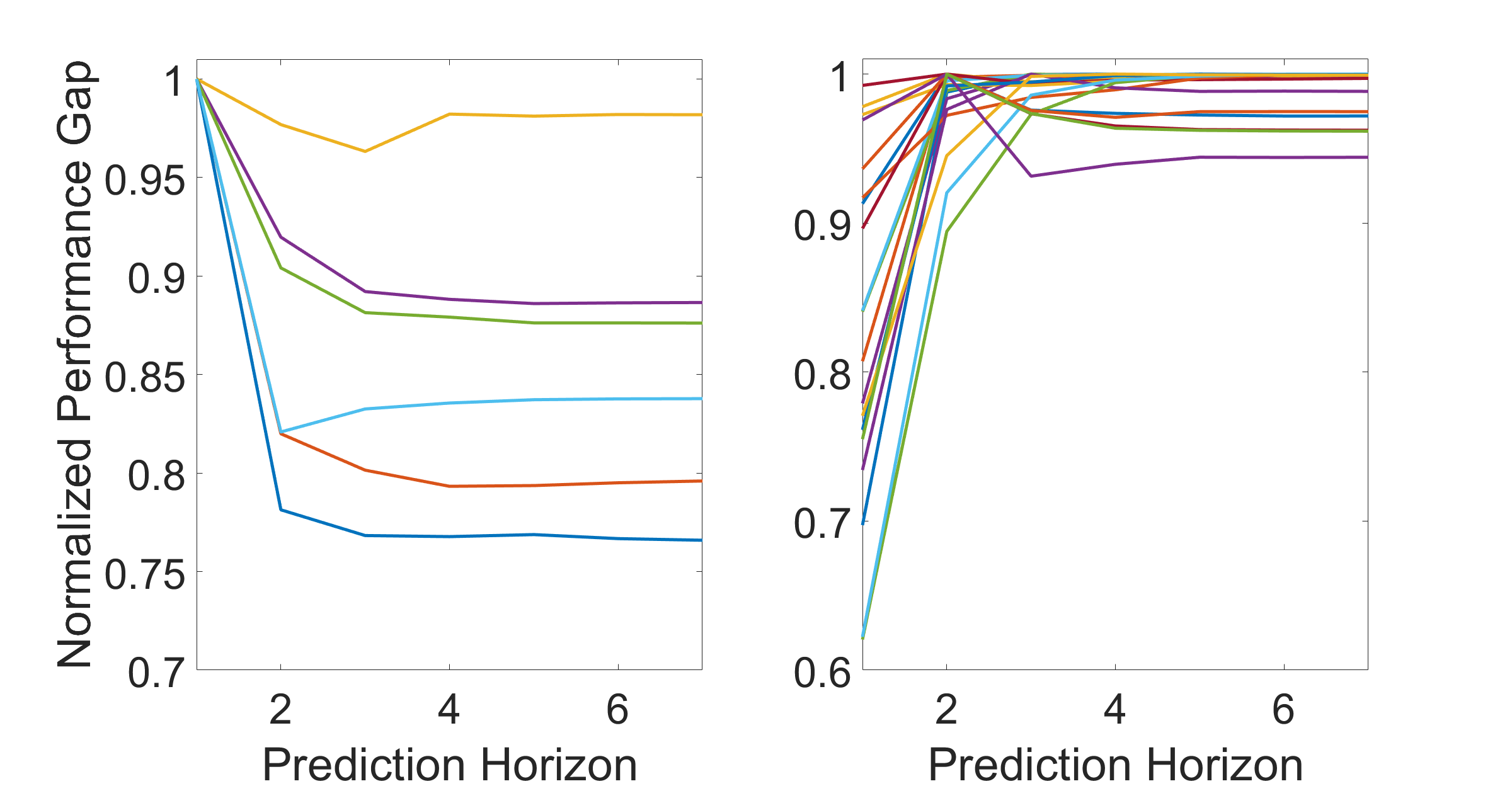
The above observation depends on the performance upper bound in (29) and thus may not reflect the actual behavior of JKRHCJKJ_{K_{\mathrm{RHC}}}-J_{K_{\star}}. However, the observation can indeed be seen in extensive simulations in Fig. 1. In this simulation study, 55 random real systems (A,B)(A_{\star},B_{\star}), with n=10n=10 and m=2m=2, are generated, where each entry in AA_{\star} and BB_{\star} is sampled from 𝒰[2,2]\mathcal{U}_{[-2,2]} and 𝒰[0,1]\mathcal{U}_{[0,1]}, respectively. All systems have controllability index ncr=5n_{\mathrm{cr}}=5. Moreover, each (A,B)(A_{\star},B_{\star}) and the corresponding PP_{\star} are perturbed by random matrices555For PP_{\star}, a random matrix is multiplied by its transpose to generate a positive semi-definite matrix perturbation., whose entries are sampled from 𝒰[0,0.001]\mathcal{U}_{[0,0.001]}. This is repeated for 55 times for each real system, leading to 2525 approximate (A^,B^,P)(\hat{A},\hat{B},P) and 2525 nominal RHC controllers. For each controller, we vary its prediction horizon and compute the normalized performance gap as [JKRHC(N)JK]/maxN(JKRHC(N)JK)[J_{K_{\mathrm{RHC}}}(N)-J_{K_{\star}}]/\max_{N}(J_{K_{\mathrm{RHC}}}(N)-J_{K_{\star}}).

The results are shown in Fig. 1. The performance gaps have initial transient behaviors but converge fast as NN increases. Most controllers indeed obtain their optimal control performance by choosing N=1N=1 or the largest NN until convergence. Moreover, all of them converge after N>ncrN>n_{\mathrm{cr}}. This shows the potential benefit of choosing a finite NN satisfying N>ncrN>n_{\mathrm{cr}}, even if NN\to\infty is desired. This is particularly important when the computational aspect is taken into account, as a larger NN also leads to a higher computational cost.

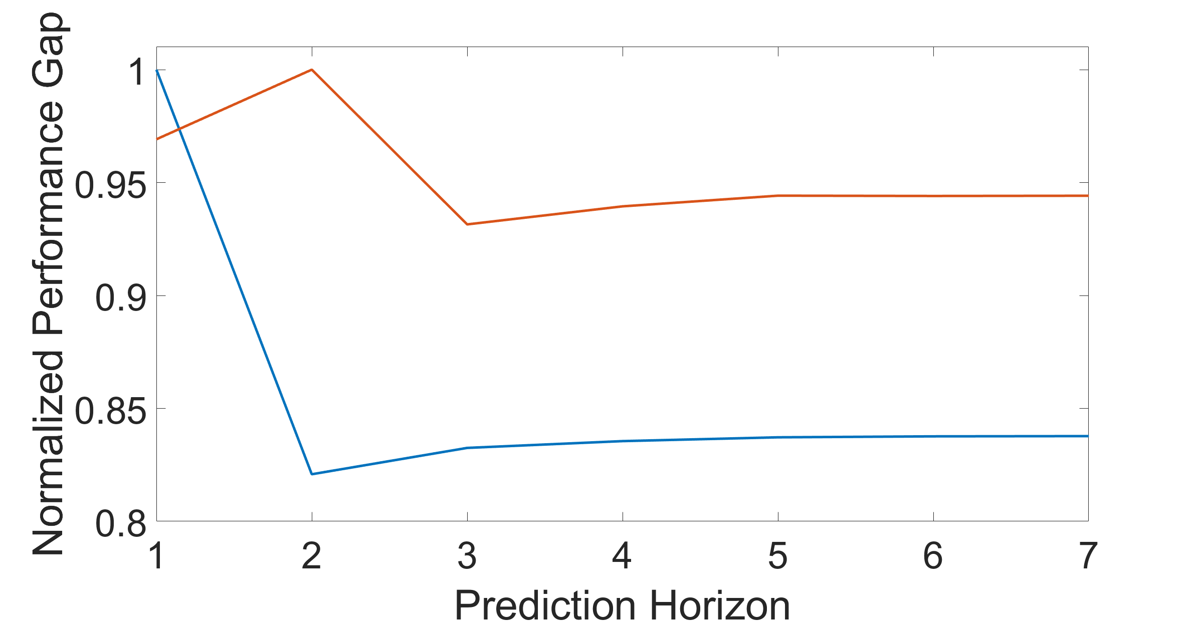
However, there are a few cases where the optimal NN is finite but greater than 11. Two examples are shown in Fig. 2, where N=2N=2 and N=3N=3 achieve the optimal performance, respectively. However, the performance difference between the optimal performance and the performance upon convergence is not significant. These examples show that the upper bound may not reflect the actual behavior of JKRHCJKJ_{K_{\mathrm{RHC}}}-J_{K_{\star}}.

Refer to caption
Fig. 1: Given 1010-dimensional random real systems, the performance gaps JKRHCJKJ_{K_{\mathrm{RHC}}}-J_{K_{\star}} (after normalization) of 2525 nominal RHC controllers under varying NN are divided into two groups based on the trend of their performance and are shown in these two figures.
Refer to caption
Fig. 2: Two nominal RHC controllers achieve their optimal closed-loop performance at N=2N=2 and N=3N=3, respectively.
Remark 5

Lemma 7 is established under a tight condition, i.e., the bound 1/(40Υ4P2)1/(40\Upsilon_{\star}^{4}\|P_{\star}\|^{2}) on the errors can be small. This is a common limitation of analytical error bounds [19, 20]. Despite this limitation, we can still obtain a non-trivial result in Theorem 3, and this result can be observed when going beyond the tight condition, e.g., the modeling errors of the simulation in Fig. 1 are actually greater than 1/(40Υ4P2)1/(40\Upsilon_{\star}^{4}\|P_{\star}\|^{2}).

To better interpret Theorem 3, we also consider the practical case where P=0P=0 in the RHC controller (3). Then we have the following result.

Corollary 1

Given the nominal RHC controller (3) with P=0P=0, if Assumptions 1, 2, 4, and 5 hold, and if εm+E^(εm,P,N1)1/(40Υ4P2)\varepsilon_{\mathrm{m}}+\widehat{E}(\varepsilon_{\mathrm{m}},\|P_{\star}\|,N-1)\leqslant 1/(40\Upsilon_{\star}^{4}\|P_{\star}\|^{2}), then ABKRHCA_{\star}-B_{\star}K_{\mathrm{RHC}} is Schur stable with JKRHCJKg(εm,εp,N)J_{K_{\mathrm{RHC}}}-J_{K_{\star}}\leqslant g(\varepsilon_{\mathrm{m}},\varepsilon_{\mathrm{p}},N), where infNg(εm,εp,N)=limNg(εm,εp,N)\inf_{N}g(\varepsilon_{\mathrm{m}},\varepsilon_{\mathrm{p}},N)=\lim_{N\to\infty}g(\varepsilon_{\mathrm{m}},\varepsilon_{\mathrm{p}},N) and g(εm,εp,N)g(\varepsilon_{\mathrm{m}},\varepsilon_{\mathrm{p}},N) is strictly decreasing as NN increases.

The above result shows that for the RHC controller with zero terminal function, using a large prediction horizon, ideally the nominal LQR controller, is beneficial. This is because the other choice N=1N=1 leads to KRHC=0K_{\mathrm{RHC}}=0, which will never stabilize the system if the system is open-loop unstable.

5 Extensions to stabilizable systems

We generalize the previous results for controllable systems to stabilizable systems. Without controllability to establish the fast decay rates 1β1-\beta_{\star} in (18) and γ2\gamma_{2} in (26) for incri\geqslant n_{\mathrm{cr}}, we only establish a single decay rate for all i1i\geqslant 1. These results for stabilizable systems are formalized in Appendix 11. The single decay rate greatly simplifies the analysis, which leads to a variant of Theorem 2 for stabilizable systems:

Theorem 4

If Assumptions 2, 3, and 4(a) hold, then for i+i\in\mathbb{Z}^{+}, A^,B^(i)(P)P\|\mathcal{R}^{(i)}_{\hat{A},\hat{B}}(P)-P_{\star}\|

E^sta(εm,εp,i)ζ¯{γ1iγ¯2iεp+ψ~(εm)[j=0i1γ¯2jγ1j]},\leqslant\widehat{E}_{\mathrm{sta}}(\varepsilon_{\mathrm{m}},\varepsilon_{\mathrm{p}},i)\triangleq\overline{\zeta}\bigg{\{}\gamma_{1}^{i}\overline{\gamma}_{2}^{i}\varepsilon_{\mathrm{p}}+\tilde{\psi}(\varepsilon_{\mathrm{m}})\Big{[}\sum_{j=0}^{i-1}\overline{\gamma}_{2}^{j}\gamma_{1}^{j}\Big{]}\bigg{\}}, (33)

where γ1\gamma_{1} defined in (25), ψ~\tilde{\psi} is defined in (54) and satisfies ψ~=O(εm)\tilde{\psi}=O(\varepsilon_{\mathrm{m}}), and ζ¯\overline{\zeta}, γ¯2\overline{\gamma}_{2} are defined in Proposition 1.

Similarly to (29), (33) also leads to an error bound

gsta(εm,εp,N)c[εm+E^sta(εm,εp,N1)]2.g_{\mathrm{sta}}(\varepsilon_{\mathrm{m}},\varepsilon_{\mathrm{p}},N)\triangleq c_{\star}[\varepsilon_{\mathrm{m}}+\widehat{E}_{\mathrm{sta}}(\varepsilon_{\mathrm{m}},\varepsilon_{\mathrm{p}},N-1)]^{2}. (34)

Equation (33) can be rewritten as (30). Therefore, the observation from Theorem 3 that the performance upper bound achieves its infimum at N=1N=1 or NN\to\infty remains valid for stabilizble systems, now depending on the sign of (31) only.

By observing (17), we note that for stabilizable systems, the faster rate 1β1-\beta_{\star} in (18) can also be established by letting ii be sufficiently large, e.g. larger than a constant i0i_{0}, such that the closed-loop matrices in ΦA,B(0:i)(P)\Phi^{(0:i)}_{A,B}(P) become close to LL_{\star} in (10). However, i0i_{0} can be large and also does not have a clear interpretation, unlike the controllability index ncrn_{\mathrm{cr}} in (18). Therefore, this technical extension is not pursued here.

6 Applications in learning-based control

Besides the obtained theoretical insights, our suboptimality analysis can also be used to analyze the performance of learning-based controllers. Results in this section generalize the results in [19, 18, 20] for learning-based LQR controllers with an infinite horizon to RHC controllers with an arbitrary prediction horizon. We will compare our performance bounds analytically with the above existing results, as is done in similar studies on regret analysis [19, 20].

6.1 Offline identification and control

In this subsection, we first obtain an estimate (A^,B^)(\hat{A},\hat{B}) offline from measured data of the unknown real system (2), and then synthesize a controller (3) with zero terminal matrix P=0P=0. This is the classical receding-horizon LQ controller [10].

There are many recent studies on linear system identification and its finite-sample error bounds [22, 23, 18]. For interpretability, we consider a relatively simple estimator from [18]. Assume that the white noise wtw_{t} is Gaussian, and we conduct TT independent experiments on the unknown real system (2) by injecting independent Gaussian noise, i.e., ut𝒩(0,σu2I)u_{t}\sim\mathcal{N}(0,\sigma_{u}^{2}I) with σu>0\sigma_{u}>0, where each experiment starts from x0=0x_{0}=0 and lasts for tht_{h} time steps. This leads to the measured data {(xt(l),ut(l))}t=0th\{(x_{t}^{(l)},u_{t}^{(l)})\}_{t=0}^{t_{h}}, l=1,,Tl=1,\dots,T, which is independent over the experiment index ll. To avoid the dependence among the data for establishing the estimation error, we use one data sample from each independent experiment, and then an estimate (A^,B^)(\hat{A},\hat{B}) is obtained from the least-squares (LS) estimator [18]:

[A^B^]=argminA,Bl=1Txth(l)[AB][xth1(l)uth1(l)]2.\begin{bmatrix}\hat{A}&\hat{B}\end{bmatrix}=\arg\min_{A,B}\sum_{l=1}^{T}\Big{\|}x_{t_{h}}^{(l)}-\begin{bmatrix}A&B\end{bmatrix}\begin{bmatrix}x_{t_{h}-1}^{(l)}\\ u_{t_{h}-1}^{(l)}\end{bmatrix}\Big{\|}^{2}. (35)

An error bound εm\varepsilon_{\mathrm{m}} can be obtained [18, Prop. 1] such that with high probability and for some constant cls>0c_{\mathrm{ls}}>0 that depends on system parameters,

max{A^A,B^B}εm=cls/T.\max\{\|\hat{A}-A_{\star}\|,\|\hat{B}-B_{\star}\|\}\leqslant\varepsilon_{\mathrm{m}}=c_{\mathrm{ls}}/\sqrt{T}. (36)

Consider the nominal controller (3) with P=0P=0 and (A^,B^)(\hat{A},\hat{B}) from (35). We can provide an end-to-end control performance guarantee by combining the LS estimation error bound (36) and our performance bound (34). We consider (34) here for generality as it needs more relaxed assumptions than (29). To this end, we first simplify (34) for interpretability.

Proposition 2

Given the controller (3) with P=0P=0, if Assumptions 2, 3, and 4(a) hold, and if εm+E^sta(εm,P,N1)1/(40Υ4P2)\varepsilon_{\mathrm{m}}+\widehat{E}_{\mathrm{sta}}(\varepsilon_{\mathrm{m}},\|P_{\star}\|,N-1)\leqslant 1/(40\Upsilon_{\star}^{4}\|P_{\star}\|^{2}), then ABKRHCA_{\star}-B_{\star}K_{\mathrm{RHC}} is Schur stable with

JKRHCJKC(μN1+εm)2,J_{K_{\mathrm{RHC}}}-J_{K_{\star}}\leqslant C\left(\mu_{\star}^{N-1}+\varepsilon_{\mathrm{m}}\right)^{2},

for some C>0C>0 that is independent of NN and εm\varepsilon_{\mathrm{m}}, where μ1β/(2)3/2(0,1)\mu_{\star}\triangleq\sqrt{1-\beta_{\star}/(2)^{3/2}}\in(0,1).

Combining Proposition 2 with the estimation error bound (36) from [18] directly leads to the following end-to-end performance guarantee:

Corollary 2

Consider the estimate (A^,B^)(\hat{A},\hat{B}) from the estimator (35) and the controller (3) with P=0P=0. If Assumptions 1, 2 hold, and if the noise wtw_{t} is Gaussian and cls/T+E^sta(cls/T,P,N1)1/(40Υ4P2)c_{\mathrm{ls}}/\sqrt{T}+\widehat{E}_{\mathrm{sta}}(c_{\mathrm{ls}}/\sqrt{T},\|P_{\star}\|,N-1)\leqslant 1/(40\Upsilon_{\star}^{4}\|P_{\star}\|^{2}), then for any δ(0,1)\delta\in(0,1), there exists a sufficiently large TT such that with probability at least 1δ1-\delta, ABKRHCA_{\star}-B_{\star}K_{\mathrm{RHC}} is Schur stable with

JKRHCJKC(μN1+log(1/δ)/T)2,J_{K_{\mathrm{RHC}}}-J_{K_{\star}}\leqslant C\left(\mu_{\star}^{N-1}+\sqrt{\log(1/\delta)/T}\right)^{2},

for some C>0C>0 that is independent of NN and TT.

Corollary 2 reveals the effect of the prediction horizon and the number of data samples on the control performance. The performance gap is O(1/T)O(1/T) if NN\to\infty, i.e., when the nominal LQR controller is considered. This growth rate agrees with the recent study [19] of the LQR controller. When NN is finite, an additional error μN1\mu_{\star}^{N-1} exists and decreases as NN increases. When TT\to\infty, the estimated model converges to the real system with high probability, leading to performance gap O(μN1)O(\mu_{\star}^{N-1}), i.e., the performance of the controller converges exponentially to the optimal one as NN increases, which matches our observation in (20). Note that controllability in Assumption 1 is introduced in Corollary 2, required by the estimation error bound [18]. Moreover, Assumption 4(a) is absent, as it is satisfied by a sufficiently large TT.

Remark 6

We have used data from multiple independent experiments for estimating the model; however, in practice, maybe only one experiment can be conducted. In this case, an LS estimator with the data from a single experiment can be used, with its error bound studied in [22, 23].

6.2 Online learning control with regret bound

In this subsection, we consider the adaptive LQR controller algorithm in [20], which has a state-of-the-art regret guarantee with greedy exploration. While there are other exploration strategies [17], the more fundamental greedy exploration is chosen to demonstrate the application of our analysis.

The nominal LQR controller within the adaptive control scheme in [20] is replaced by the receding-horizon LQ controller (3) with P=0P=0. Other cost matrices QQ and RR are fixed throughout the close-loop operation. To match the setting in [20], in this subsection, we assume that wtw_{t} is Gaussian with σw=1\sigma_{w}=1 and the initial condition is x0=0x_{0}=0. Following [20], we assume that a stabilizing but possibly suboptimal controller gain K0K_{0} for the unknown true system is given a priori.

We briefly introduce the main idea of [20, Algorithm 1], and the details can be found in [20]. Starting from x0=0x_{0}=0 and a random input u0𝒩(0,I)u_{0}\sim\mathcal{N}(0,I), the control algorithm utilizes a fixed controller gain KkK_{k} within each time step period [tk,tk+1)[t_{k},t_{k+1}), where tk=2k1t_{k}=2^{k-1} and k{1,2,}k\in\{1,2,\dots\} is the period index. In the first few periods, the gain K0K_{0} with a Gaussian perturbation is used, i.e., ut=Kkxt+gtu_{t}=-K_{k}x_{t}+g_{t} with Kk=K0K_{k}=K_{0} and gt𝒩(0,I)g_{t}\sim\mathcal{N}(0,I), to stabilize the unknown system. The perturbation gtg_{t} ensures the informativity of the data for estimating the system later.

After collecting sufficient data at time step tk0t_{k_{0}} for some period k0k_{0}, the controller conducts the following steps for every period kk0k\geqslant k_{0}. A new model (A^k,B^k)(\hat{A}_{k},\hat{B}_{k}) is re-estimated at the initial time step tkt_{k} of period kk. It is obtained from the LS estimator using the data {zt}t=tk1tk1\{z_{t}\}_{t=t_{k-1}}^{t_{k}-1} from the last period k1k-1, where zt[xtut]z_{t}\triangleq\begin{bmatrix}x_{t}^{\top}&u_{t}^{\top}\end{bmatrix}^{\top}, as

[A^kB^k]=argminA,Bt=tk1tk1xt+1[AB]zt2.\begin{bmatrix}\hat{A}_{k}&\hat{B}_{k}\end{bmatrix}=\arg\min_{A,B}\sum_{t=t_{k-1}}^{t_{k}-1}\Big{\|}x_{t+1}-\begin{bmatrix}A&B\end{bmatrix}z_{t}\Big{\|}^{2}. (37)

Then, for t[tk,tk+1)t\in[t_{k},t_{k+1}), the algorithm employs a new RHC controller gain KRHC,kK_{\mathrm{RHC},k}, formulated based on666In [20], the estimated model, if not accurate, is further modified via projection. These details are presented in [20]. This projection step is redundant if the estimated model is sufficiently accurate. Moreover, it relies on a conservative error bound, leading to practical issues as discussed in Section 6.3. Therefore, the projection step is ignored later in the simulations of Section 6.3. (A^k,B^k)(\hat{A}_{k},\hat{B}_{k}) via either the implicit form (3) or the explicit form (6), with a random perturbation, i.e., ut=KRHC,kxt+σkgtu_{t}=-K_{\mathrm{RHC},k}x_{t}+\sigma_{k}g_{t}, where σk>0\sigma_{k}>0 determines the size of the perturbation and decays as kk increases.

In this case, let TT denote the total number of time steps that have passed, and let kTk_{T} denote the final period index. Let 𝒞:nm\mathcal{C}:\mathbb{R}^{n}\to\mathbb{R}^{m} denote the above adaptive controller, and its performance is typically characterized by regret [22, 33]:

Regret(T)t=0T[xtQxt+𝒞(xt)R𝒞(xt)JK],\mathrm{Regret}(T)\triangleq\sum_{t=0}^{T}\left[x_{t}^{\top}Qx_{t}+\mathcal{C}^{\top}(x_{t})R\mathcal{C}(x_{t})-J_{K_{\star}}\right],

which measures the accumulative error of a particular realization under the controller. Ideally, we would like to have a sublinear regret, such that as TT\to\infty, Regret(T)/T\mathrm{Regret}(T)/T converges to zero with high probability, i.e., the average performance of the adaptive controller is optimal.

As shown in [20, Sect. 5.1] and [20, Appendix G.2], the following holds for the considered adaptive controller with high probability:

Regret(T)=O~(k=k0kTtk(JKRHC,kJK)+T).\mathrm{Regret}(T)=\tilde{O}\left(\sum_{k=k_{0}}^{k_{T}}t_{k}(J_{K_{\mathrm{RHC},k}}-J_{K_{\star}})+\sqrt{T}\right).

Combining the above equation with Proposition 2 leads to

Regret(T)=O~(k=k0kTtk[μN1+1/(tk1/4)]2+T),\kern-3.00003pt\mathrm{Regret}(T)=\tilde{O}\left(\sum_{k=k_{0}}^{k_{T}}t_{k}\big{[}\mu_{\star}^{N-1}+1/(t_{k}^{1/4})\big{]}^{2}+\sqrt{T}\right), (38)

where we have used the fact that the estimated model, obtained at tkt_{k}, has error εm=O(1/tk1/4)\varepsilon_{\mathrm{m}}=O(1/t_{k}^{1/4}) with high probability, based on [20, Lem. 5.4].

The regret upper bound (38) provides some interesting information. Firstly, note that k=k0kTtkC¯T\sum_{k=k_{0}}^{k_{T}}\sqrt{t_{k}}\leqslant\bar{C}\sqrt{T} for some constant C¯>0\bar{C}>0. Therefore, if we have an infinite prediction horizon NN\to\infty, i.e., when the nominal LQR is considered, then Regret(T)=O~(T)\mathrm{Regret}(T)=\tilde{O}(\sqrt{T}), which matches the rate of the adaptive LQR controllers in [19, 20].

If we have a finite NN, (38) shows with high probability,

Regret(T)=O~(TμN+T),\mathrm{Regret}(T)=\tilde{O}\left(T\mu_{\star}^{N}+\sqrt{T}\right), (39)

where the regret is linear in TT. This observation matches the result in [34], where the regret of a linear unconstrained RHC controller, with a fixed prediction horizon and an exact system model, is linear in TT. This linear regret is caused by the fact that even if the model is perfectly identified, the RHC controller still deviates from the optimal LQR controller due to its finite prediction horizon.

To achieve a sublinear regret, (39) suggests that an adaptive prediction horizon is preferred. As also suggested in [34] but for the case of a known system, we can update NN via

N=O(log(tk)),N=O(\log(t_{k})),

e.g., updating N=log(tk)/(4log(μ))N=\lfloor-\log(t_{k})/(4\log(\mu_{\star}))\rfloor, when the model is re-estimated, which again leads to a sublinear regret O~(T)\tilde{O}(\sqrt{T}) according to (38). Note that this is the optimal rate for the regret [20]. The intuition of this choice is that, with a more refined model due to re-estimation, the prediction horizon can be increased adaptively to improve the control performance.

6.3 Simulations of adaptive RHC

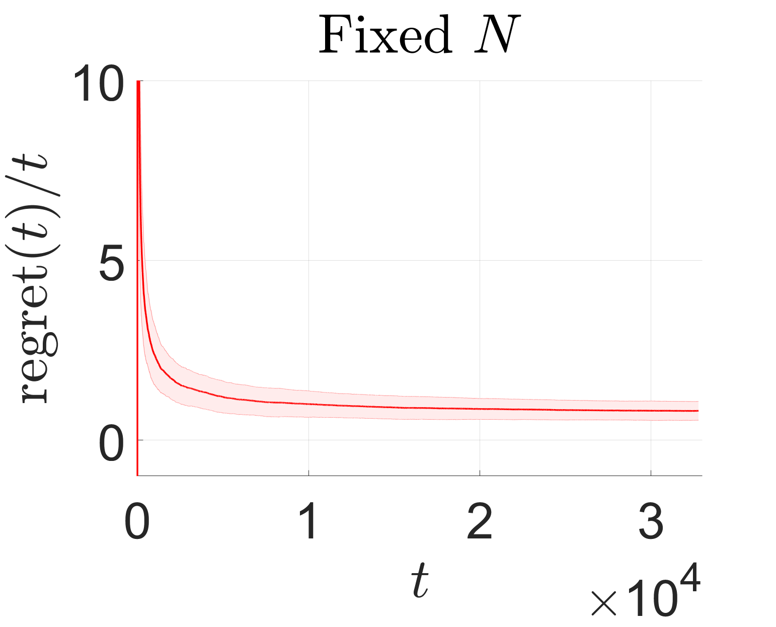
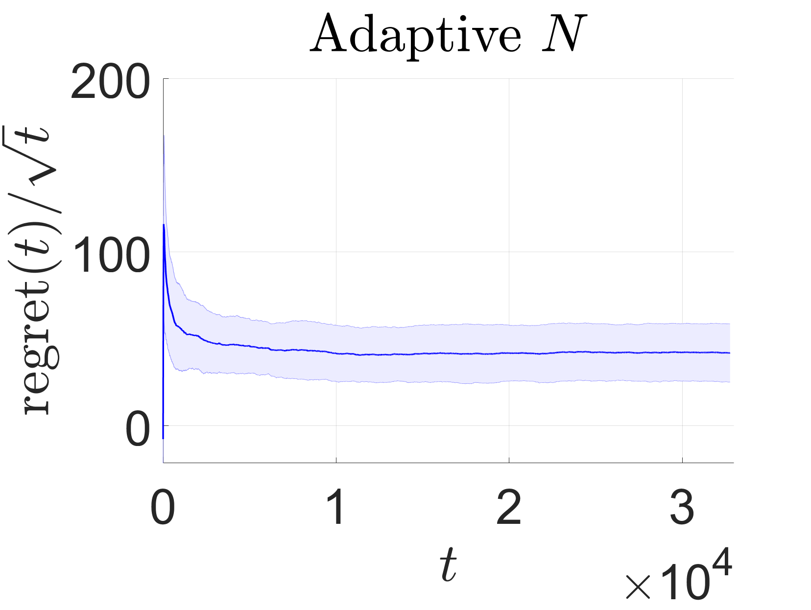
We use simulations to demonstrate the main theoretical insights from Section 6.2: For the adaptive RHC algorithm, while a fixed prediction horizon leads to a linear regret growth rate O~(T)\tilde{O}\left(T\right), an adaptive horizon, being a logarithmic function of time, leads to a more desired sublinear rate O~(T)\tilde{O}(\sqrt{T}).

While the algorithm based on [20] in Section 6.2 has a regret guarantee, a conservative analytical modeling error bound εm\varepsilon_{\mathrm{m}}, analogous to (36), is utilized in [20]. This conservatism causes practical issues, e.g., despite the actual modeling error being small, the if condition εm<δ¯(A^,B^)\varepsilon_{\mathrm{m}}<\bar{\delta}(\hat{A},\hat{B}) for some function δ¯\bar{\delta} in the algorithm is hardly met as the bound εm\varepsilon_{\mathrm{m}} is too large. Therefore, by introducing tuning parameters, we slightly modify the algorithm in Section 6.2 to avoid analytical error bounds. The resulting algorithm is more practical and suffices to demonstrate the theoretical insight. We summarize the modifications here:

  1. (i)

    The key period index k0k_{0} in Section 6.2 is chosen to be the first period kk such that t=0tk1ztztδ1I\sum_{t=0}^{t_{k}-1}z_{t}z_{t}^{\top}\succeq\delta_{1}I holds, where δ1[1,)\delta_{1}\in[1,\infty) is a tuning parameter.

  2. (ii)

    The LS estimator (37) uses data {zt}t=0tk1\{z_{t}\}_{t=0}^{t_{k}-1} from all the previous periods, instead of only the last period.

  3. (iii)

    We let σk=min{1,(δ2/tk)1/2}\sigma_{k}=\min\{1,\big{(}\delta_{2}/\sqrt{t_{k}}\big{)}^{1/2}\}, where δ2(0,)\delta_{2}\in(0,\infty) is a tuning parameter instead of being computed via an analytical formula as in [20].

In the above, (i) ensures that the collected data is informative to obtain an accurate LS estimate of the model. Point (ii) ensures the updated estimate is not worse than the previous one, as more data is used for estimation. With point (iii), the exploration effort decays as the period index increases.

We use the modified algorithm to control the unknown system with the following true system matrices:

A=[0.520.90.60.11.81.30.31.6], B=[0.310.9100.9].A_{\star}=\begin{bmatrix}0.5&-2&0.9\\ 0.6&0.1&1.8\\ 1.3&-0.3&1.6\end{bmatrix},\text{ }B_{\star}=\begin{bmatrix}0.3&1\\ 0.9&1\\ 0&0.9\end{bmatrix}.

Starting from x0=0x_{0}=0, we compare the regret growth of the adaptive RHC controller with a fixed prediction horizon N=3N=3 and the controller with an adaptive prediction horizon N=max{3,log(tk)}N=\max\{3,\lfloor\log(t_{k})\rfloor\}, where NN is updated when the controller is updated. Other parameters are σw=1\sigma_{w}=1, Q=IQ=I, R=IR=I, P=0P=0, δ1=4\delta_{1}=4, δ2=0.5\delta_{2}=0.5, and K0K_{0} is the LQR controller gain for stabilization. Note that although the true system and its LQR controller are unknown, we choose the LQR controller to be the initial controller for simplicity. The choice of K0K_{0}, if stabilizing, does not affect our illustration of the regret growth.

As the regret is a random variable due to the disturbance wtw_{t}, we conduct 100100 simulations for each controller. The regret growth over time, normalized by t\sqrt{t} or tt, is shown in Fig. 3. It shows that the regret grows linearly in TT under the fixed NN but in the order of T\sqrt{T} under the adaptive NN. This illustrates the advantage of the adaptive prediction horizon for regret minimization.

While the modified algorithm does not preserve the theoretical guarantee in Section 6.2, it remains useful to demonstrate the impact of the adaptive prediction horizon on regret growth. Moreover, this algorithm has a structure similar to that of existing algorithms with regret guarantees, e.g., the adaptive LQ Gaussian (LQG) controller in [35]. Our future work will investigate the possibility of extending existing analyses to the modified algorithm.

Refer to caption
Refer to caption
Fig. 3: For the controller with the fixed NN and the one with the adaptive NN, the mean and standard deviation (shaded region) of the normalized regrets, regret(t)/t\mathrm{regret}(t)/t for the fixed NN and regret(t)/t\mathrm{regret}(t)/\sqrt{t} for the adaptive NN, over 100100 simulations are shown. After initial transient behavior, the normalized regrets converge to positive constants.

7 Conclusions

This work analyzes the suboptimality of RHC under the joint effect of the modeling error, the terminal value function error, and the prediction horizon in the LQ setting. By deriving a novel perturbation analysis of the Riccati difference equation, we have obtained a novel performance upper bound of the controller. The bound suggests that letting the prediction horizon be 11 or ++\infty can potentially be beneficial, depending on the relative difference between the modeling error and the terminal matrix error. Moreover, when an infinite horizon is desired, a prediction horizon larger than the controllability index can be sufficient for achieving a near-optimal performance. Besides the above insight, this obtained performance bound has also been shown to be useful for analyzing the performance of learning-based receding-horizon LQ controllers.

Future work includes the derivation of tighter performance bounds to capture the non-trivial optimal horizon, which is finite but larger than 11. Moreover, the extension of the obtained results to more general settings, e.g., constrained RHC controllers with possibly nonlinear dynamics or output feedback, is an important direction. The analysis of computational efficiency is not considered in this work, as the controller in the current setting has a closed-form expression. Analyzing computational efficiency is also an important direction for the more general settings.

\appendices

8 Technical tools

Technical tools from the literature are collected here.

Lemma 8

Given 0<ab<10<a\leqslant b<1 and any positive integer ii, we have (1bi+1)/(1ai+1)(1bi)/(1ai)0.(1-b^{i+1})/(1-a^{i+1})-(1-b^{i})/(1-a^{i})\geqslant 0.

Proof 8.1.

This result is obtained by applying formula aibi=(ab)(ai1+ai2b++abi2+bi1)a^{i}-b^{i}=(a-b)(a^{i-1}+a^{i-2}b+\dots+ab^{i-2}+b^{i-1}).

Lemma 5.

([19, Lem. 7]) Given M𝕊+nM\in\mathbb{S}^{n}_{+} and N𝕊+nN\in\mathbb{S}^{n}_{+}, it holds that N(I+MN)1N\|N(I+MN)^{-1}\|\leqslant\|N\|.

Lemma 6.

([19, Lem. 5]) Consider Mn×nM\in\mathbb{R}^{n\times n}, c1c\geqslant 1, ρρ(M)\rho\geqslant\rho(M) such that Micρi\|M^{i}\|\leqslant c\rho^{i} for any i+i\in\mathbb{Z}^{+}. For any i+i\in\mathbb{Z}^{+} and Δn×n\Delta\in\mathbb{R}^{n\times n}, (M+Δ)ic(cΔ+ρ)i\|(M+\Delta)^{i}\|\leqslant c(c\|\Delta\|+\rho)^{i} holds.

Important identities from [10], [28, eq. (2.3) and (4.2)] are collected in the following result:

Lemma 7.

If R0R\succ 0, for any PP, P1P_{1}, P2𝕊+nP_{2}\in\mathbb{S}_{+}^{n} and i+i\in\mathbb{Z}^{+},

  1. (a)

    A,B(P1)A,B(P2)=[AB𝒦A,B(P1)](P1P2)[AB𝒦A,B(P2)];\mathcal{R}_{A,B}(P_{1})-\mathcal{R}_{A,B}(P_{2})=[A-B\mathcal{K}_{A,B}(P_{1})]^{\top}(P_{1}-P_{2})[A-B\mathcal{K}_{A,B}(P_{2})];

  2. (b)

    A,B(P)=[AB𝒦A,B(P)]P[AB𝒦A,B(P)]+𝒦A,B(P)R𝒦A,B(P)+Q\mathcal{R}_{A,B}(P)=[A-B\mathcal{K}_{A,B}(P)]^{\top}P[A-B\mathcal{K}_{A,B}(P)]+\mathcal{K}^{\top}_{A,B}(P)R\mathcal{K}_{A,B}(P)+Q;

  3. (c)

    (P)B(R+BPB)1B=SB(I+PSB)1\mathcal{F}(P)\triangleq B(R+B^{\top}PB)^{-1}B^{\top}=S_{B}(I+PS_{B})^{-1};

  4. (d)

    ΦA,B(0:i)(P1)=[I+𝒪A,B(i)(P1)(P2P1)]ΦA,B(0:i)(P2)\Phi^{(0:i)}_{A,B}(P_{1})=\big{[}I+\mathcal{O}_{A,B}^{(i)}(P_{1})(P_{2}-P_{1})\big{]}\Phi^{(0:i)}_{A,B}(P_{2}) with 𝒪A,B(i)\mathcal{O}_{A,B}^{(i)} defined in (41).

In addition, the following perturbation analysis of the Riccati equation from [20, Prop. 6] and [20, Lem. B.5, B.8] is useful for deriving the results of this work.

Lemma 8.

([20]) Given QQ, RR, and (A,B)(A_{\star},B_{\star}), consider any alternative system (A^,B^)(\hat{A},\hat{B}) satisfying max{A^A,B^B}εm\max\{\|\hat{A}-A_{\star}\|,\|\hat{B}-B_{\star}\|\}\leqslant\varepsilon_{\mathrm{m}}. If Assumptions 2 and 3 hold, then

  1. 1.

    PIP_{\star}\succeq I, PL2\|P_{\star}\|\geqslant\|L_{\star}\|^{2}, and PK2\|P_{\star}\|\geqslant\|K_{\star}\|^{2};

  2. 2.

    if εm<1/(8P2)\varepsilon_{\mathrm{m}}<1/(8\|P_{\star}\|^{2}), then (A^,B^)(\hat{A},\hat{B}) is stabilizable and

    P^αεmP,K^K7αεm7/2P7/2εm\|\hat{P}\|\leqslant\alpha_{\varepsilon_{\mathrm{m}}}\|P_{\star}\|,\quad\|\hat{K}-K_{\star}\|\leqslant 7\alpha_{\varepsilon_{\mathrm{m}}}^{7/2}\|P_{\star}\|^{7/2}\varepsilon_{\mathrm{m}} (40)

    where αεm=(18P2εm)1/2\alpha_{\varepsilon_{\mathrm{m}}}=(1-8\|P_{\star}\|^{2}\varepsilon_{\mathrm{m}})^{-1/2}, P^\hat{P} is the fixed point of the Riccati equation and K^\hat{K} is the LQR control gain for (A^,B^)(\hat{A},\hat{B}).

Another tool is the stability analysis of time-varying systems, directly implied by the proof of [29, Thm. 23.3].

Lemma 9.

Consider a system x¯k+1=Akx¯k\bar{x}_{k+1}=A_{k}\bar{x}_{k} with Akn×nA_{k}\in\mathbb{R}^{n\times n} and ϕ(j:i)Ai1Aj\phi^{(j:i)}\triangleq A_{i-1}\dots A_{j} for integers ij0i\geqslant j\geqslant 0. If there exists a matrix sequence Wk𝕊nW_{k}\in\mathbb{S}^{n} satisfying for k[j,i]k\in[j,i]

blIWkbuI, and AkWk+1AkWkaI,\displaystyle b_{\mathrm{l}}I\preceq W_{k}\preceq b_{\mathrm{u}}I,\text{ and }A_{k}^{\top}W_{k+1}A_{k}-W_{k}\preceq-aI,

for some positive constants blb_{\mathrm{l}}, bub_{\mathrm{u}}, and aa, then ϕ(j:i)bu/bl(1a/bu)ij\|\phi^{(j:i)}\|\leqslant\sqrt{b_{\mathrm{u}}/b_{\mathrm{l}}}\big{(}\sqrt{1-a/b_{\mathrm{u}}}\big{)}^{i-j} with a/bu(0,1]a/b_{\mathrm{u}}\in(0,1].

9

9.1 Proof of Lemma 1

Lemma 7(b) shows σ¯(Q)ILPLP-\underline{\sigma}(Q)I\succeq L_{\star}^{\top}P_{\star}L_{\star}-P_{\star}, and in addition, we have σ¯(Q)Iσ¯(P)IPσ¯(P)I\underline{\sigma}(Q)I\preceq\underline{\sigma}(P_{\star})I\preceq P_{\star}\preceq\overline{\sigma}(P_{\star})I. Then the direct application of Lemma 9 proves the result. Note that β<1\beta_{\star}<1 holds; otherwise, P=QP_{\star}=Q and thus A=0A=0 based on Lemma 7(b), which contradicts with Assumption 2.

9.2 Proof of Lemma 3

We first define the following Gramian matrix: for i1i\geqslant 1

𝒪A,B(i)(P)k=0i1A,Bk(P(k))(P(k))[A,Bk(P(k))],\mathcal{O}_{A,B}^{(i)}(P)\triangleq\sum_{k=0}^{i-1}\mathcal{L}^{k}_{A,B}(P^{(k)})\mathcal{F}\big{(}P^{(k)}\big{)}[\mathcal{L}^{k}_{A,B}(P^{(k)})]^{\top}, (41)

where (P)B(R+BPB)1B\mathcal{F}(P)\triangleq B(R+B^{\top}PB)^{-1}B^{\top}, 𝒪A,B(0)(P)0\mathcal{O}_{A,B}^{(0)}(P)\triangleq 0, and recall that P(i)P^{(i)} is a shorthand notation for A,B(i)(P)\mathcal{R}^{(i)}_{A,B}(P).

The proof for the case incri\geqslant n_{\mathrm{cr}} is achieved based on Lemma 3 and [28, Lem. 4.1]. We highlight the key steps for completeness. If incri\geqslant n_{\mathrm{cr}}, matrix 𝒪A,B(i)(P)\mathcal{O}_{A_{\star},B_{\star}}^{(i)}(P_{\star}) has full rank due to Assumption 1. Lemma 7(d) shows [I+𝒪A,B(i)(P)(PP)]ΦA,B(0:i)(P)=Li\big{[}I+\mathcal{O}_{A_{\star},B_{\star}}^{(i)}(P_{\star})(P-P_{\star})\big{]}\Phi^{(0:i)}_{A_{\star},B_{\star}}(P)=L_{\star}^{i} for i+i\in\mathbb{Z}^{+}. Then based on Assumption 2 and [28, Lem. 4.1], I+𝒪A,B(i)(P)(PP)I+\mathcal{O}_{A_{\star},B_{\star}}^{(i)}(P_{\star})(P-P_{\star}) is non-singular for incri\geqslant n_{\mathrm{cr}}, and moreover, its inverse is uniformly upper bounded for any incri\geqslant n_{\mathrm{cr}} and any P0P\succeq 0. Combining (17) and the above shows for incri\geqslant n_{\mathrm{cr}}, A,B(i)(P)P=(Li)[I+𝒪A,B(i)(P)(PP)](PP)Li,\mathcal{R}^{(i)}_{A_{\star},B_{\star}}(P)-P_{\star}=(L_{\star}^{i})^{\top}\big{[}I+\mathcal{O}_{A_{\star},B_{\star}}^{(i)}(P_{\star})(P-P_{\star})\big{]}^{-\top}(P-P_{\star})L_{\star}^{i}, which together with (11) concludes the proof for incri\geqslant n_{\mathrm{cr}}, with

τβ1supP𝕊+nsupincr[I+𝒪A,B(i)(P)(PP)]1.\tau_{\star}\triangleq\beta_{\star}^{-1}\sup_{P\in\mathbb{S}^{n}_{+}}\sup_{i\geqslant n_{\mathrm{cr}}}\big{\|}\big{[}I+\mathcal{O}_{A_{\star},B_{\star}}^{(i)}(P_{\star})(P-P_{\star})\big{]}^{-1}\big{\|}. (42)

When 1i<ncr1\leqslant i<n_{\mathrm{cr}}, the rank of the controllability matrix is less than nn, and thus 𝒪A,B(i)(P)\mathcal{O}_{A_{\star},B_{\star}}^{(i)}(P_{\star}) is not guaranteed to be of full rank. Then directly exploiting (17) leads to

A,B(i)(P)PΦA,B(0:i)(P)LiPP.\displaystyle\|\mathcal{R}^{(i)}_{A_{\star},B_{\star}}(P)-P_{\star}\|\leqslant\|\Phi^{(0:i)}_{A_{\star},B_{\star}}(P)\|\|L_{\star}^{i}\|\|P-P_{\star}\|. (43)

A naive approach is to upper bound ΦA,B(0:i)(P)\|\Phi^{(0:i)}_{A_{\star},B_{\star}}(P)\| by a constant. However, due to QIQ\succeq I, ΦA,B(0:i)(P)\Phi^{(0:i)}_{A_{\star},B_{\star}}(P) can also be shown to be exponentially decay as ii increases, even without the controllability property. This result in (74) is exploited here and proved later in Appendix 11. Combining (11), (43), and (74) proves this case, with

τ¯Υ3(1+Υ+P)β1(P+Υβ1)(1β)1,\overline{\tau}_{\star}\triangleq\Upsilon_{\star}^{3}(1+\Upsilon_{\star}+\|P_{\star}\|)\sqrt{\beta_{\star}^{-1}(\|P_{\star}\|+\Upsilon_{\star}\beta_{\star}^{-1})(1-\beta_{\star})^{-1}}, (44)

derived from (74) using Υεp\Upsilon_{\star}\geqslant\varepsilon_{\mathrm{p}}. The case i=0i=0 holds trivially due to τ¯1\overline{\tau}_{\star}\geqslant 1.

9.3 Proof of Lemma 4

The result is based on the following lemma:

Lemma 10.

For any F𝕊+nF\in\mathbb{S}^{n}_{+} with FPε\|F-P_{\star}\|\leqslant\varepsilon, if Assumption 2 and 3 hold, and if Υε\Upsilon_{\star}\geqslant\varepsilon, then K=𝒦A^,B^(F)K=\mathcal{K}_{\hat{A},\hat{B}}(F) satisfies

KKΥ2(P+1)(3εm+4ε)σ¯(R).\|K-K_{\star}\|\leqslant\frac{\Upsilon_{\star}^{2}(\sqrt{\|P_{\star}\|}+1)(3\varepsilon_{\mathrm{m}}+4\varepsilon)}{\underline{\sigma}(R)}. (45)
Proof 9.1.

Standard algebraic reformulations show B^FB^BPBεm2ε+2εmεΥ+Pεm2+2εmΥP+εΥ24Υ2ε+3ΥPεm,\|\hat{B}^{\top}F\hat{B}-B_{\star}^{\top}P_{\star}B_{\star}\|\leqslant\varepsilon_{\mathrm{m}}^{2}\varepsilon+2\varepsilon_{\mathrm{m}}\varepsilon\Upsilon_{\star}+\|P_{\star}\|\varepsilon_{\mathrm{m}}^{2}+2\varepsilon_{\mathrm{m}}\Upsilon_{\star}\|P_{\star}\|+\varepsilon\Upsilon_{\star}^{2}\leqslant 4\Upsilon_{\star}^{2}\varepsilon+3\Upsilon_{\star}\|P_{\star}\|\varepsilon_{\mathrm{m}}, where the last inequality uses Υmax{εm,ε}\Upsilon_{\star}\geqslant\max\{\varepsilon_{\mathrm{m}},\varepsilon\}. Then following [19, Lem. 2] analogously, we have for any xx, σ¯(R)(KK)x(4Υ2ε+3ΥPεm)(K+1)xΥ2(4ε+3εm)(P+1)x,\underline{\sigma}(R)\|(K-K_{\star})x\|\leqslant(4\Upsilon_{\star}^{2}\varepsilon+3\Upsilon_{\star}\|P_{\star}\|\varepsilon_{\mathrm{m}})(\|K_{\star}\|+1)\|x\|\leqslant\Upsilon_{\star}^{2}(4\varepsilon+3\varepsilon_{\mathrm{m}})(\sqrt{\|P_{\star}\|}+1)\|x\|, where the last inequality follows from Lemma 8.

Then Lemma 4 can be proved as follows. Firstly, based on (45) and the assumption, we have B(KK)8Υ4(εm+ε)/σ¯(R)1/5P3/2\|B_{\star}(K-K_{\star})\|\leqslant 8\Upsilon_{\star}^{4}(\varepsilon_{\mathrm{m}}+\varepsilon)/\underline{\sigma}(R)\leqslant 1/5\|P_{\star}\|^{-3/2}. Then given Assumption 2, we have ΣKσw2P\|\Sigma_{K_{\star}}\|\leqslant\sigma_{w}^{2}\|P_{\star}\| based on [20, Lem. B.5]777Note that in this work, the noise wtw_{t} has a covariance matrix σw2I\sigma_{w}^{2}I instead of II as in [20]; however, the results in [20] extends to this work trivially.. Therefore, B(KK)1/5P3/2\|B_{\star}(K-K_{\star})\|\leqslant 1/5\|P_{\star}\|^{-3/2} implies B(KK)1/5σw3ΣK3/2\|B_{\star}(K-K_{\star})\|\leqslant 1/5\sigma_{w}^{3}\|\Sigma_{K_{\star}}\|^{-3/2}, which further shows that ABKA_{\star}-B_{\star}K is Schur stable, according to [20, Lem. B.12]. Then given a stabilizing KK and based on [19, Lem. 3], we have

JKJKΣKR+BPBKKF2\displaystyle J_{K}-J_{K_{\star}}\leqslant\|\Sigma_{K}\|\|R+B_{\star}^{\top}P_{\star}B_{\star}\|\|K-K_{\star}\|_{F}^{2}
2ΣKR+BPBKK2min{n,m}\displaystyle\leqslant 2\|\Sigma_{K_{\star}}\|\|R+B_{\star}^{\top}P_{\star}B_{\star}\|\|K-K_{\star}\|^{2}\min\{n,m\}
2min{n,m}σw2(σ¯(R)+Υ3)PKK2,\displaystyle\leqslant 2\min\{n,m\}\sigma_{w}^{2}(\overline{\sigma}(R)+\Upsilon_{\star}^{3})\|P_{\star}\|\|K-K_{\star}\|^{2},

where the second inequality holds due to ΣK2ΣK\|\Sigma_{K}\|\leqslant 2\|\Sigma_{K_{\star}}\| under B(KK)1/5σw3ΣK3/2\|B_{\star}(K-K_{\star})\|\leqslant 1/5\sigma_{w}^{3}\|\Sigma_{K_{\star}}\|^{-3/2} according to [20, Lem. B.12]. Then combining the above result and Lemma 10 concludes the proof.

9.4 Proof of Lemma 5

Define the shorthand notations S^SB^\hat{S}\triangleq S_{\hat{B}} and SSBS_{\star}\triangleq S_{B_{\star}}. We prove this result by induction. The equality holds trivially when i=0i=0. Assume it holds for i=ki=k, then

P^(k+1)P(k+1)=A^,B^(k)(P^(1))A,B(k)(P(1))=\displaystyle\hat{P}^{(k+1)}-P_{\star}^{(k+1)}=\mathcal{R}^{(k)}_{\hat{A},\hat{B}}\big{(}\hat{P}^{(1)}\big{)}-\mathcal{R}^{(k)}_{A_{\star},B_{\star}}\big{(}P_{\star}^{(1)}\big{)}=
[ΦA^,B^(0:k)(P^(1))](P^(1)P(1))Φ¯(0:k)(P(1))+\displaystyle\big{[}\Phi_{\hat{A},\hat{B}}^{(0:k)}(\hat{P}^{(1)})\big{]}^{\top}(\hat{P}^{(1)}-P_{\star}^{(1)})\bar{\Phi}^{(0:k)}(P_{\star}^{(1)})+
j=1k[ΦA^,B^(kj+1:k)(P^(1))](P^(kj+1),P(kj+1))\displaystyle\sum_{j=1}^{k}\big{[}\Phi_{\hat{A},\hat{B}}^{(k-j+1:k)}(\hat{P}^{(1)})\big{]}^{\top}\mathcal{M}\Big{(}\hat{P}^{(k-j+1)},P_{\star}^{(k-j+1)}\Big{)}
×Φ¯(kj+1:k)(P(1))\displaystyle\times\bar{\Phi}^{(k-j+1:k)}(P_{\star}^{(1)})
=\displaystyle= [ΦA^,B^(1:k+1)(P1)](P^(1)P(1))Φ¯(1:k+1)(P2)+\displaystyle\big{[}\Phi_{\hat{A},\hat{B}}^{(1:k+1)}(P_{1})\big{]}^{\top}(\hat{P}^{(1)}-P_{\star}^{(1)})\bar{\Phi}^{(1:k+1)}(P_{2})+ (46a)
j=1k[ΦA^,B^(kj+2:k+1)(P1)](P^(kj+1),P(kj+1))\displaystyle\sum_{j=1}^{k}\big{[}\Phi_{\hat{A},\hat{B}}^{(k-j+2:k+1)}(P_{1})\big{]}^{\top}\mathcal{M}\Big{(}\hat{P}^{(k-j+1)},P_{\star}^{(k-j+1)}\Big{)} (46b)
×Φ¯(kj+2:k+1)(P2)\displaystyle\times\bar{\Phi}^{(k-j+2:k+1)}(P_{2}) (46c)

In (46), it holds that P^(1)P(1)\hat{P}^{(1)}-P_{\star}^{(1)}

=A^P1(I+S^P1)1A^AP2(I+SP2)1A\displaystyle=\hat{A}^{\top}P_{1}(I+\hat{S}P_{1})^{-1}\hat{A}-A_{\star}^{\top}P_{2}(I+S_{\star}P_{2})^{-1}A_{\star}
=A^[P1(I+S^P1)1P2(I+SP2)1]A^Term I+\displaystyle=\underbrace{\hat{A}^{\top}[P_{1}(I+\hat{S}P_{1})^{-1}-P_{2}(I+S_{\star}P_{2})^{-1}]\hat{A}}_{\text{Term I}}+ (47)
A^P2(I+SP2)1A^AP2(I+SP2)1ATerm II,\displaystyle\underbrace{\hat{A}^{\top}P_{2}(I+S_{\star}P_{2})^{-1}\hat{A}-A_{\star}^{\top}P_{2}(I+S_{\star}P_{2})^{-1}A_{\star}}_{\text{Term II}}, (48)

where Term I further leads to A^[P1(I+S^P1)1P2(I+SP2)1]A^=A^[(I+P1S^)1P1P2(I+SP2)1]A^=A^(I+P1S^)1[P1(I+SP2)(I+P1S^)P2](I+SP2)1A^=A^(I+P1S^)1[(P1P2)+(P1SP2P1S^P2)](I+SP2)1A^=A^(I+P1S^)1(P1P2)[I+(SS^)P2](I+SP2)1A^+A^(I+P1S^)1P2(SS^)P2(I+SP2)1A^\hat{A}^{\top}[P_{1}(I+\hat{S}P_{1})^{-1}-P_{2}(I+S_{\star}P_{2})^{-1}]\hat{A}=\hat{A}^{\top}[(I+P_{1}\hat{S})^{-1}P_{1}-P_{2}(I+S_{\star}P_{2})^{-1}]\hat{A}=\hat{A}^{\top}(I+P_{1}\hat{S})^{-1}[P_{1}(I+S_{\star}P_{2})-(I+P_{1}\hat{S})P_{2}](I+S_{\star}P_{2})^{-1}\hat{A}=\hat{A}^{\top}(I+P_{1}\hat{S})^{-1}[(P_{1}-P_{2})+(P_{1}S_{\star}P_{2}-P_{1}\hat{S}P_{2})](I+S_{\star}P_{2})^{-1}\hat{A}=\hat{A}^{\top}(I+P_{1}\hat{S})^{-1}(P_{1}-P_{2})[I+(S_{\star}-\hat{S})P_{2}](I+S_{\star}P_{2})^{-1}\hat{A}+\hat{A}^{\top}(I+P_{1}\hat{S})^{-1}P_{2}(S_{\star}-\hat{S})P_{2}(I+S_{\star}P_{2})^{-1}\hat{A}

=\displaystyle= [A^,B^(P1)](P1P2)¯(P2)+\displaystyle[\mathcal{L}_{\hat{A},\hat{B}}(P_{1})]^{\top}(P_{1}-P_{2})\bar{\mathcal{L}}(P_{2})+ (49a)
A^(I+P1S^)1P2(SS^)P2(I+SP2)1A^\displaystyle\hat{A}^{\top}(I+P_{1}\hat{S})^{-1}P_{2}(S_{\star}-\hat{S})P_{2}(I+S_{\star}P_{2})^{-1}\hat{A} (49b)

combining (48) and (49) leads to

P^(1)P(1)=[A^,B^(P1)](P1P2)¯(P2)+(P1,P2).\hat{P}^{(1)}-P_{\star}^{(1)}=[\mathcal{L}_{\hat{A},\hat{B}}(P_{1})]^{\top}(P_{1}-P_{2})\bar{\mathcal{L}}(P_{2})+\mathcal{M}(P_{1},P_{2}). (50)

Finally, plugging (50) into (46) shows P^(k+1)P(k+1)\hat{P}^{(k+1)}-P_{\star}^{(k+1)} also satisfies the equality in this lemma, which concludes the proof by induction.

9.5 Proof of Lemma 6

The matrix ¯(P)\bar{\mathcal{L}}(P_{\star}) in (22) is reformulated as

¯(P)=L+(P)+SΔP[(P)+L]Δ,\bar{\mathcal{L}}(P_{\star})=L_{\star}+\underbrace{\mathcal{H}(P_{\star})+S_{\Delta}P_{\star}[\mathcal{H}(P_{\star})+L_{\star}]}_{\Delta\triangleq}, (51)

where SΔ=SBSB^S_{\Delta}=S_{B_{\star}}-S_{\hat{B}}. To upper bound the norm of Δ\Delta, we first upper bound (P)\mathcal{H}(P_{\star}): (P)=[IB(R+BPB)1BP](A^A)(1+B2P(R+BPB)1)εm(1+Υ2P)εm,\|\mathcal{H}(P_{\star})\|=\|[I-B_{\star}(R+B_{\star}^{\top}P_{\star}B_{\star})^{-1}B_{\star}^{\top}P_{\star}](\hat{A}-A_{\star})\|\leqslant(1+\|B_{\star}\|^{2}\|P_{\star}\|\|(R+B_{\star}^{\top}P_{\star}B_{\star})^{-1}\|)\varepsilon_{\mathrm{m}}\leqslant(1+\Upsilon_{\star}^{2}\|P_{\star}\|)\varepsilon_{\mathrm{m}}, where the first identity follows form the matrix inverse lemma, and the final step follows from R+BPBRIR+B_{\star}^{\top}P_{\star}B_{\star}\succeq R\succeq I due to Assumption 2. Due to RIR\succeq I, letting εs=SΔ\varepsilon_{s}=\|S_{\Delta}\| leads to

εs=SBSB^εm2+2Υεm, and \varepsilon_{s}=\|S_{B_{\star}}-S_{\hat{B}}\|\leqslant\varepsilon_{\mathrm{m}}^{2}+2\Upsilon_{\star}\varepsilon_{\mathrm{m}},\text{ and } (52)
Δ(1+Υ2P)εm+εsP((P)+L)\displaystyle\|\Delta\|\leqslant(1+\Upsilon_{\star}^{2}\|P_{\star}\|)\varepsilon_{\mathrm{m}}+\varepsilon_{s}\|P_{\star}\|(\|\mathcal{H}(P_{\star})\|+\|L_{\star}\|)
(1+Υ2P)εm+εsP[(1+Υ2P)εm+P]\displaystyle\leqslant(1+\Upsilon_{\star}^{2}\|P_{\star}\|)\varepsilon_{\mathrm{m}}+\varepsilon_{s}\|P_{\star}\|\big{[}(1+\Upsilon_{\star}^{2}\|P_{\star}\|)\varepsilon_{\mathrm{m}}+\|P_{\star}\|\big{]}
ψ(εm)εm{1+Υ2P+\displaystyle\leqslant\psi(\varepsilon_{\mathrm{m}})\triangleq\varepsilon_{\mathrm{m}}\Big{\{}1+\Upsilon_{\star}^{2}\|P_{\star}\|+
(εm+2Υ)[(P+Υ2P2)εm+P2]}\displaystyle(\varepsilon_{\mathrm{m}}+2\Upsilon_{\star})[(\|P_{\star}\|+\Upsilon_{\star}^{2}\|P_{\star}\|^{2})\varepsilon_{\mathrm{m}}+\|P_{\star}\|^{2}\big{]}\Big{\}} (53)
=O(εm),\displaystyle=O(\varepsilon_{\mathrm{m}}),

where we have used LP\|L_{\star}\|\leqslant\|P_{\star}\| from Lemma 8 in the second inequality. Based on (11) and Φ¯(j:i)(P)=¯(P)ij=(L+Δ)ij\bar{\Phi}^{(j:i)}(P_{\star})=\bar{\mathcal{L}}(P_{\star})^{i-j}=(L_{\star}+\Delta)^{i-j}, applying Lemma 6 concludes the proof.

9.6 Proof of Theorem 2

Based on (23), we first upper bound \mathcal{M} and then combine it with Lemma 6 and Proposition 1. Recall (52), and for any P𝕊+nP\in\mathbb{S}^{n}_{+},

(P,P)(A^A)P(I+SBP)1(A^A)\displaystyle\|\mathcal{M}(P,P_{\star})\|\leqslant\|(\hat{A}-A_{\star})^{\top}P_{\star}(I+S_{B_{\star}}P_{\star})^{-1}(\hat{A}-A_{\star})
+AP(I+SBP)1(A^A)\displaystyle+A_{\star}^{\top}P_{\star}(I+S_{B_{\star}}P_{\star})^{-1}(\hat{A}-A_{\star})
+(A^A)P(I+SBP)1A\displaystyle+(\hat{A}-A_{\star})^{\top}P_{\star}(I+S_{B_{\star}}P_{\star})^{-1}A_{\star}\|
+A^P2A^,B^(P)εs\displaystyle+\|\hat{A}\|\|P_{\star}\|^{2}\|\mathcal{L}_{\hat{A},\hat{B}}(P)\|\varepsilon_{s}
P(εm2+2Υεm)+(εm+Υ)4P2(1+P)εs\displaystyle\leqslant\|P_{\star}\|(\varepsilon_{\mathrm{m}}^{2}+2\Upsilon_{\star}\varepsilon_{\mathrm{m}})+(\varepsilon_{\mathrm{m}}+\Upsilon_{\star})^{4}\|P_{\star}\|^{2}(1+\|P\|)\varepsilon_{s}
ψ~(εm)(εm2+2Υεm)\displaystyle\leqslant\tilde{\psi}(\varepsilon_{\mathrm{m}})\triangleq(\varepsilon_{\mathrm{m}}^{2}+2\Upsilon_{\star}\varepsilon_{\mathrm{m}})
×[P+(εm+Υ)4P2(1+P+Υ)],\displaystyle\times\big{[}\|P_{\star}\|+(\varepsilon_{\mathrm{m}}+\Upsilon_{\star})^{4}\|P_{\star}\|^{2}(1+\|P_{\star}\|+\Upsilon_{\star})\big{]}, (54)

where (78) and Lemma 5 are used, and ψ~(εm)=O(εm)\tilde{\psi}(\varepsilon_{\mathrm{m}})=O(\varepsilon_{\mathrm{m}}).

Then if incri\geqslant n_{\mathrm{cr}}, combining (23), (24), (26) and (54) shows P^(i)Pζ~εpγ2iγ1i+ζ~ψ~{k=0ncr1γ¯2kγ1k+k=ncri1γ2kγ1k}.\|\hat{P}^{(i)}-P_{\star}\|\leqslant\tilde{\zeta}\varepsilon_{\mathrm{p}}\gamma_{2}^{i}\gamma_{1}^{i}+\tilde{\zeta}\tilde{\psi}\Big{\{}\sum_{k=0}^{n_{\mathrm{cr}}-1}\overline{\gamma}_{2}^{k}\gamma_{1}^{k}+\sum_{k=n_{\mathrm{cr}}}^{i-1}\gamma_{2}^{k}\gamma_{1}^{k}\Big{\}}. Similarly, when i<ncri<n_{\mathrm{cr}}, we have P^(i)Pζ~εpγ¯2iγ1i+ζ~ψ~k=0i1γ¯2kγ1k.\|\hat{P}^{(i)}-P_{\star}\|\leqslant\tilde{\zeta}\varepsilon_{\mathrm{p}}\overline{\gamma}_{2}^{i}\gamma_{1}^{i}+\tilde{\zeta}\tilde{\psi}\sum_{k=0}^{i-1}\overline{\gamma}_{2}^{k}\gamma_{1}^{k}. Combining these two cases proves the result.

9.7 Proof of Lemma 7

We have E^ζ~ψ~2εmΥ4P2\widehat{E}\geqslant\tilde{\zeta}\tilde{\psi}\geqslant 2\varepsilon_{\mathrm{m}}\Upsilon_{\star}^{4}\|P_{\star}\|^{2}, due to

ζ~ζ¯Υ3P, and ψ~2εmΥP,\tilde{\zeta}\geqslant\overline{\zeta}\geqslant\Upsilon_{\star}^{3}\|P_{\star}\|,\text{ and }\tilde{\psi}\geqslant 2\varepsilon_{\mathrm{m}}\Upsilon_{\star}\|P_{\star}\|, (55)

which are obtained from (79) and (54). The assumption εm+E^(εm,εp,N1)1/(40Υ4P2)\varepsilon_{\mathrm{m}}+\widehat{E}(\varepsilon_{\mathrm{m}},\varepsilon_{\mathrm{p}},N-1)\leqslant 1/(40\Upsilon_{\star}^{4}\|P_{\star}\|^{2}) implies εm1/(80Υ8P4)\varepsilon_{\mathrm{m}}\leqslant 1/(80\Upsilon_{\star}^{8}\|P_{\star}\|^{4}). Then (25) and the definition of ψ\psi in (53) show ψεm9Υ3P21/(8Υ5P2)\psi\leqslant\varepsilon_{\mathrm{m}}9\Upsilon_{\star}^{3}\|P_{\star}\|^{2}\leqslant 1/(8\Upsilon_{\star}^{5}\|P_{\star}\|^{2})

<12P3/21(1+1β)β1β1=11ββ1\displaystyle<\frac{1}{2\|P_{\star}\|^{3/2}}\leqslant\frac{1}{(1+\sqrt{1-\beta_{\star}})\sqrt{\beta_{\star}^{-1}}\beta_{\star}^{-1}}=\frac{1-\sqrt{1-\beta_{\star}}}{\sqrt{\beta_{\star}^{-1}}} (56)
γ1<1,\displaystyle\implies\gamma_{1}<1,

where we use 1β<1\sqrt{1-\beta_{\star}}<1 and β1P\beta_{\star}^{-1}\leqslant\|P_{\star}\|. combining Lemma 4 and Theorem 2 concludes the proof, as the conditions in these two results are satisfied by εm1/(80Υ8P4)\varepsilon_{\mathrm{m}}\leqslant 1/(80\Upsilon_{\star}^{8}\|P_{\star}\|^{4}).

9.8 Proof of Theorem 3

Equation (27) can be written more compactly as

E^=\displaystyle\widehat{E}= ζ~{(εpψ~1γ1γ2)γ2N1γ1N1+ψ~γ1ncrγ2ncr1γ1γ2\displaystyle\tilde{\zeta}\Big{\{}\Big{(}\varepsilon_{\mathrm{p}}-\frac{\tilde{\psi}}{1-\gamma_{1}\gamma_{2}}\Big{)}\gamma_{2}^{N-1}\gamma_{1}^{N-1}+\frac{\tilde{\psi}\gamma_{1}^{n_{\mathrm{cr}}}\gamma_{2}^{n_{\mathrm{cr}}}}{1-\gamma_{1}\gamma_{2}}
+ψ~k=0ncr1γ¯2kγ1k} if N1ncr.\displaystyle+\tilde{\psi}\sum_{k=0}^{n_{\mathrm{cr}}-1}\overline{\gamma}_{2}^{k}\gamma_{1}^{k}\Big{\}}\text{ if }N-1\geqslant n_{\mathrm{cr}}. (57)

Moreover, we can quantify the change from N1<ncrN-1<n_{\mathrm{cr}} to N1ncrN-1\geqslant n_{\mathrm{cr}} by computing ΔE^E^(εm,εp,ncr)E^(εm,εp,ncr1)\Delta\widehat{E}\triangleq\widehat{E}(\varepsilon_{\mathrm{m}},\varepsilon_{\mathrm{p}},n_{\mathrm{cr}})-\widehat{E}(\varepsilon_{\mathrm{m}},\varepsilon_{\mathrm{p}},n_{\mathrm{cr}}-1)

=ζ~εp(γ1ncrγ2ncrγ1ncr1γ¯2ncr1)+ψ~ζ~γ1ncr1γ¯2ncr1\displaystyle=\tilde{\zeta}\varepsilon_{\mathrm{p}}\big{(}\gamma_{1}^{n_{\mathrm{cr}}}\gamma_{2}^{n_{\mathrm{cr}}}-\gamma_{1}^{n_{\mathrm{cr}}-1}\overline{\gamma}_{2}^{n_{\mathrm{cr}}-1}\big{)}+\tilde{\psi}\tilde{\zeta}\gamma_{1}^{n_{\mathrm{cr}}-1}\overline{\gamma}_{2}^{n_{\mathrm{cr}}-1}
=ζ~(γ1γ2)ncr1{εp[γ2γ1(γ¯2/γ2)ncr1]+ψ~(γ¯2/γ2)ncr1}.\displaystyle=\tilde{\zeta}(\gamma_{1}\gamma_{2})^{n_{\mathrm{cr}}-1}\big{\{}\varepsilon_{\mathrm{p}}[\gamma_{2}\gamma_{1}-(\overline{\gamma}_{2}/\gamma_{2})^{n_{\mathrm{cr}}-1}]+\tilde{\psi}(\overline{\gamma}_{2}/\gamma_{2})^{n_{\mathrm{cr}}-1}\big{\}}.

The above equation and γ2γ¯2\gamma_{2}\leqslant\overline{\gamma}_{2} from (26) show that

ΔE^0 iff εpψ~1γ1γ2(γ¯2/γ2)ncr10.\Delta\widehat{E}\geqslant 0\text{ iff }\varepsilon_{\mathrm{p}}-\frac{\tilde{\psi}}{1-\frac{\gamma_{1}\gamma_{2}}{(\overline{\gamma}_{2}/\gamma_{2})^{n_{\mathrm{cr}}-1}}}\leqslant 0. (58)

The statement (a) follows from (30), (32), (57), and (58). For statement (b), if 0>εpψ~/(1γ1γ2)0>\varepsilon_{\mathrm{p}}-\tilde{\psi}/(1-\gamma_{1}\gamma_{2}), then (30), (32), and (57) show that gg and E^\widehat{E} are strictly increasing as N{1,ncr}N\in\{1,\dots n_{\mathrm{cr}}\} increases, and they are also strictly increasing as Nncr+1N\geqslant n_{\mathrm{cr}}+1 increases. For the transition of the two regions of NN, consider E^(εm,εp,0)E^(εm,εp,ncr)\widehat{E}(\varepsilon_{\mathrm{m}},\varepsilon_{\mathrm{p}},0)-\widehat{E}(\varepsilon_{\mathrm{m}},\varepsilon_{\mathrm{p}},n_{\mathrm{cr}})

=εpζ~εpζ~(γ1γ2)ncrζ~ψ~1(γ1γ¯2)ncr1γ1γ¯2=ζ~[1(γ1γ2)ncr]\displaystyle=\varepsilon_{\mathrm{p}}\tilde{\zeta}-\varepsilon_{\mathrm{p}}\tilde{\zeta}(\gamma_{1}\gamma_{2})^{n_{\mathrm{cr}}}-\tilde{\zeta}\tilde{\psi}\frac{1-(\gamma_{1}\overline{\gamma}_{2})^{n_{\mathrm{cr}}}}{1-\gamma_{1}\overline{\gamma}_{2}}=\tilde{\zeta}[1-(\gamma_{1}\gamma_{2})^{n_{\mathrm{cr}}}]
×{εpψ~1γ1γ2(1γ1γ2)[1(γ1γ¯2)ncr](1γ1γ¯2)[1(γ1γ2)ncr]}\displaystyle\times\Big{\{}\varepsilon_{\mathrm{p}}-\frac{\tilde{\psi}}{1-\gamma_{1}\gamma_{2}}\frac{(1-\gamma_{1}\gamma_{2})[1-(\gamma_{1}\overline{\gamma}_{2})^{n_{\mathrm{cr}}}]}{(1-\gamma_{1}\overline{\gamma}_{2})[1-(\gamma_{1}\gamma_{2})^{n_{\mathrm{cr}}}]}\Big{\}}
ζ~[1(γ1γ2)ncr](εpψ~1γ1γ2)<0,\displaystyle\leqslant\tilde{\zeta}[1-(\gamma_{1}\gamma_{2})^{n_{\mathrm{cr}}}]\Big{(}\varepsilon_{\mathrm{p}}-\frac{\tilde{\psi}}{1-\gamma_{1}\gamma_{2}}\Big{)}<0,

where the first inequality follows from Lemma 8. The above shows argminNE^(εm,εp,N1)=argminNg(εm,εp,N)=1\arg\min_{N}\widehat{E}(\varepsilon_{\mathrm{m}},\varepsilon_{\mathrm{p}},N-1)=\arg\min_{N}g(\varepsilon_{\mathrm{m}},\varepsilon_{\mathrm{p}},N)=1. Moreover, under the additional condition εpψ~/[1γ1γ2/γratio]<0\varepsilon_{\mathrm{p}}-\tilde{\psi}/[1-\gamma_{1}\gamma_{2}/\gamma_{\mathrm{ratio}}]<0, the last part of statement (b) is proved by observing (58).

For statement (c), if εpψ~/(1γ1γ2)>0>εpψ~/(1γ1γ¯2)\varepsilon_{\mathrm{p}}-\tilde{\psi}/(1-\gamma_{1}\gamma_{2})>0>\varepsilon_{\mathrm{p}}-\tilde{\psi}/(1-\gamma_{1}\overline{\gamma}_{2}), (30) and (57) show that gg is increasing as N{1,,ncr}N\in\{1,\dots,n_{\mathrm{cr}}\} increases and decreasing as Nncr+1N\geqslant n_{\mathrm{cr}}+1 increases. This means that infNg(εm,εp,N)\inf_{N}g(\varepsilon_{\mathrm{m}},\varepsilon_{\mathrm{p}},N) equals either g(εm,εp,1)g(\varepsilon_{\mathrm{m}},\varepsilon_{\mathrm{p}},1) or limNg(εm,εp,N)\lim_{N\to\infty}g(\varepsilon_{\mathrm{m}},\varepsilon_{\mathrm{p}},N) depending on the sign of E^(εm,εp,0)limNE^(εm,εp,N)=\widehat{E}(\varepsilon_{\mathrm{m}},\varepsilon_{\mathrm{p}},0)-\lim_{N\to\infty}\widehat{E}(\varepsilon_{\mathrm{m}},\varepsilon_{\mathrm{p}},N)=

ζ~{εpψ~1γ1γ2[(1γ1γ2)[1(γ¯2γ1)ncr]1γ1γ¯2+(γ1γ2)ncr𝒱(ncr)]},\displaystyle\tilde{\zeta}\bigg{\{}\varepsilon_{\mathrm{p}}-\frac{\tilde{\psi}}{1-\gamma_{1}\gamma_{2}}\Big{[}\underbrace{\frac{(1-\gamma_{1}\gamma_{2})[1-(\overline{\gamma}_{2}\gamma_{1})^{n_{\mathrm{cr}}}]}{1-\gamma_{1}\overline{\gamma}_{2}}+(\gamma_{1}\gamma_{2})^{n_{\mathrm{cr}}}}_{\mathcal{V}(n_{\mathrm{cr}})}\Big{]}\bigg{\}},

which can be proved to be in the interval [ζ~(εpψ~/(1γ1γ¯2)),ζ~(εpψ~/(1γ1γ2))][\tilde{\zeta}(\varepsilon_{\mathrm{p}}-\tilde{\psi}/(1-\gamma_{1}\overline{\gamma}_{2})),\tilde{\zeta}(\varepsilon_{\mathrm{p}}-\tilde{\psi}/(1-\gamma_{1}\gamma_{2}))] as follows. The upper bound of this interval is proved by showing 𝒱(i+1)𝒱(i)0\mathcal{V}(i+1)-\mathcal{V}(i)\geqslant 0 and thus 𝒱(ncr)𝒱(1)=1\mathcal{V}(n_{\mathrm{cr}})\geqslant\mathcal{V}(1)=1, and the lower bound can be proved similarly. The above proves statement (c). Statement (d) follows trivially from (30) and (57).

9.9 Proof of Corollary 1

When P=0P=0, we let εp=P\varepsilon_{\mathrm{p}}=\|P_{\star}\|. According to Theorem 3, the goal is to prove Pψ~/(1γ1γ¯2)>0\|P_{\star}\|-\tilde{\psi}/(1-\gamma_{1}\overline{\gamma}_{2})>0 under the conditions. Due to ζ~ζ¯1\tilde{\zeta}\geqslant\overline{\zeta}\geqslant 1, ψ~E^1/(40Υ4P2)\tilde{\psi}\leqslant\widehat{E}\leqslant 1/(40\Upsilon_{\star}^{4}\|P_{\star}\|^{2}) holds, given the condition and (27). Based on ψ1/(8Υ5P2)\psi\leqslant 1/(8\Upsilon_{\star}^{5}\|P_{\star}\|^{2}) from (56), we have from (25) that γ1Pψ+1β<1/8Υ5P3/2.\gamma_{1}\leqslant\sqrt{\|P_{\star}\|}\psi+\sqrt{1-\beta_{\star}}<1/8\Upsilon_{\star}^{5}\|P_{\star}\|^{3/2}. This leads to

1γ1ψ~>118Υ5P3/2140Υ4P2>0,\displaystyle 1-\gamma_{1}-\tilde{\psi}>1-\frac{1}{8\Upsilon_{\star}^{5}\|P_{\star}\|^{3/2}}-\frac{1}{40\Upsilon_{\star}^{4}\|P_{\star}\|^{2}}>0,

and ψ~/(1γ1)<1\tilde{\psi}/(1-\gamma_{1})<1. Finally, P1\|P_{\star}\|\geqslant 1 from Lemma 8 implies

Pψ~1γ1γ¯21ψ~1γ1>0,\displaystyle\|P_{\star}\|-\frac{\tilde{\psi}}{1-\gamma_{1}\overline{\gamma}_{2}}\geqslant 1-\frac{\tilde{\psi}}{1-\gamma_{1}}>0, (59)

which together with Theorem 3 concludes the proof.

9.10 Proof of Proposition 2

Since P=0P=0, we let εp=P\varepsilon_{\mathrm{p}}=\|P_{\star}\|. In addition, εm1/(16P2)\varepsilon_{\mathrm{m}}\leqslant 1/(16\|P_{\star}\|^{2}) holds under the assumption, which leads to

αεm[1,2],\alpha_{\varepsilon_{\mathrm{m}}}\in[1,\sqrt{2}], (60)

and thus γ¯2μ<1\overline{\gamma}_{2}\leqslant\mu_{\star}<1. Therefore, we have

E^staζ~{PμN1+ψ~/(1μ)}.\displaystyle\widehat{E}_{\mathrm{sta}}\leqslant\tilde{\zeta}\Big{\{}\|P_{\star}\|\mu_{\star}^{N-1}+\tilde{\psi}/(1-\mu_{\star})\Big{\}}. (61)

Given the upper bound on εm\varepsilon_{\mathrm{m}}, ψ~\tilde{\psi} in (54) satisfies ψ~C1εm\tilde{\psi}\leqslant C_{1}\varepsilon_{\mathrm{m}} for some constant C1C_{1} independent of NN and εm\varepsilon_{\mathrm{m}}, and ζ~\tilde{\zeta} can also be upper bounded by some constant C2C_{2}. This shows E^staC2max{P,C1/(1γ1μ)}[μN1+εm].\widehat{E}_{\mathrm{sta}}\leqslant C_{2}\max\{\|P_{\star}\|,C_{1}/(1-\gamma_{1}\mu_{\star})\}[\mu_{\star}^{N-1}+\varepsilon_{\mathrm{m}}]. Combining the above inequality with (29) concludes the proof.

10 Proof of Proposition 1

To prove this result, the dual Riccati mapping is relevant:

dual(P)\displaystyle\mathcal{R}_{\mathrm{dual}}(P)\triangleq AP(I+QP)1A+SB,\displaystyle A_{\star}P(I+QP)^{-1}A_{\star}^{\top}+S_{B_{\star}}, (62)

and its fixed point is denoted by PdualP_{\mathrm{dual}}. Let P^dual\hat{P}_{\mathrm{dual}} be a fixed point of (62) with (A,B)(A_{\star},B_{\star}) replaced by (A^,B^)(\hat{A},\hat{B}). Let L^\hat{L} be the closed-loop system for (A^,B^)(\hat{A},\hat{B}) under the corresponding LQR controller.

We will prove this result by considering the case ijncri-j\geqslant n_{\mathrm{cr}} and the case ij<ncri-j<n_{\mathrm{cr}} separately. When ijncri-j\geqslant n_{\mathrm{cr}}, the overall proof strategy is as follows. Due to ΦA^,B^(j:i)(P)=ΦA^,B^(0:ij)(P^(j))\Phi_{\hat{A},\hat{B}}^{(j:i)}(P)=\Phi_{\hat{A},\hat{B}}^{(0:i-j)}(\hat{P}^{(j)}), Lemma 7(d) shows [I+𝒪A^,B^(ij)(P^)(P^(j)P^)]ΦA^,B^(j:i)(P)=L^ij\big{[}I+\mathcal{O}_{\hat{A},\hat{B}}^{(i-j)}(\hat{P})(\hat{P}^{(j)}-\hat{P})\big{]}\Phi^{(j:i)}_{\hat{A},\hat{B}}(P)=\hat{L}^{i-j} for i+i\in\mathbb{Z}^{+}. Moreover, [28, Lem. 4.1] shows that if 𝒪A^,B^(ij)(P^)\mathcal{O}_{\hat{A},\hat{B}}^{(i-j)}(\hat{P}) is positive definite, we have

ΦA^,B^(j:i)(P)=[I+𝒪A^,B^(ij)(P^)(P^(j)P^)]1L^ij\displaystyle\|\Phi^{(j:i)}_{\hat{A},\hat{B}}(P)\|=\|\big{[}I+\mathcal{O}_{\hat{A},\hat{B}}^{(i-j)}(\hat{P})(\hat{P}^{(j)}-\hat{P})\big{]}^{-1}\hat{L}^{i-j}\|
[𝒪A^,B^(ij)(P^)]1P^dualL^ij,\displaystyle\leqslant\|[\mathcal{O}_{\hat{A},\hat{B}}^{(i-j)}(\hat{P})]^{-1}\|\|\hat{P}_{\mathrm{dual}}\|\|\hat{L}^{i-j}\|, (63)

Then the proof consists of the following analysis:

  • Perturbation analysis of the closed-loop system L^\hat{L};

  • Perturbation analysis of the Gramian matrix: Show that 𝒪A^,B^(ij)(P^)\mathcal{O}_{\hat{A},\hat{B}}^{(i-j)}(\hat{P}) is invertible for ijncri-j\geqslant n_{\mathrm{cr}} and provides an upper bound on [𝒪A^,B^(ij)(P^)]1\|[\mathcal{O}_{\hat{A},\hat{B}}^{(i-j)}(\hat{P})]^{-1}\|;

  • Perturbation analysis of P^dual\|\hat{P}_{\mathrm{dual}}\|.

All perturbation bounds resulting from the above analysis will be expressed as functions of εm\varepsilon_{\mathrm{m}} and εp\varepsilon_{\mathrm{p}}.

The decay rate of the perturbed closed-loop system can be obtained as follows. Given QIQ\succeq I, combining (11) and Lemma 8 leads to

L^ijσ¯(P^)/σ¯(Q)(1σ¯(Q)/σ¯(P^))ij\displaystyle\|\hat{L}^{i-j}\|\leqslant\sqrt{\overline{\sigma}(\hat{P})/\underline{\sigma}(Q)}\Big{(}\sqrt{1-\underline{\sigma}(Q)/\overline{\sigma}(\hat{P})}\Big{)}^{i-j}
αεmβ1(1αεm1β)ij.\displaystyle\leqslant\sqrt{\alpha_{\varepsilon_{\mathrm{m}}}\beta_{\star}^{-1}}\Big{(}\sqrt{1-\alpha_{\varepsilon_{\mathrm{m}}}^{-1}\beta_{\star}}\Big{)}^{i-j}. (64)

The remaining analysis is presented as follows.

10.1 Perturbation analysis of the Gramian matrix

If ijncri-j\geqslant n_{\mathrm{cr}}, then 𝒪A^,B^(ij)(P^)𝒪A^,B^(ncr)(P^)\mathcal{O}_{\hat{A},\hat{B}}^{(i-j)}(\hat{P})\succeq\mathcal{O}_{\hat{A},\hat{B}}^{(n_{\mathrm{cr}})}(\hat{P}) and

𝒪A^,B^(ncr)(P^)(R+B^P^B^)1𝒞ncr(L^,B^)[𝒞ncr(L^,B^)].\mathcal{O}_{\hat{A},\hat{B}}^{(n_{\mathrm{cr}})}(\hat{P})\succeq(\|R+\hat{B}^{\top}\hat{P}\hat{B}\|)^{-1}\mathcal{C}_{n_{\mathrm{cr}}}(\hat{L},\hat{B})\big{[}\mathcal{C}_{n_{\mathrm{cr}}}(\hat{L},\hat{B})\big{]}^{\top}.

The Gramian matrix 𝒞ncr(L^,B^)[𝒞ncr(L^,B^)]\mathcal{C}_{n_{\mathrm{cr}}}(\hat{L},\hat{B})[\mathcal{C}_{n_{\mathrm{cr}}}(\hat{L},\hat{B})]^{\top} is a perturbed version of 𝒞ncr(L,B)[𝒞ncr(L,B)]\mathcal{C}_{n_{\mathrm{cr}}}(L_{\star},B_{\star})[\mathcal{C}_{n_{\mathrm{cr}}}(L_{\star},B_{\star})]^{\top}. Based on Lemma 8, we can upper bound the perturbation of LL_{\star} as

L^LAA^+(B^B)(K^K)\displaystyle\|\hat{L}-L_{\star}\|\leqslant\|A_{\star}-\hat{A}\|+\|(\hat{B}-B_{\star})(\hat{K}-K_{\star})\|
+(B^B)K+B(K^K)\displaystyle+\|(\hat{B}-B_{\star})K_{\star}\|+\|B_{\star}(\hat{K}-K_{\star})\|
εLεm[1+7αεm7/2P7/2(εm+Υ)+P1/2],\displaystyle\leqslant\varepsilon_{L}\triangleq\varepsilon_{\mathrm{m}}\big{[}1+7\alpha_{\varepsilon_{\mathrm{m}}}^{7/2}\|P_{\star}\|^{7/2}(\varepsilon_{\mathrm{m}}+\Upsilon_{\star})+\|P_{\star}\|^{1/2}\big{]}, (65)

which satisfies

εL=O(εm).\varepsilon_{L}=O(\varepsilon_{\mathrm{m}}). (66)

Under Assumption 1, recall σ¯(𝒞ncr(L,B))ν\underline{\sigma}(\mathcal{C}_{n_{\mathrm{cr}}}(L_{\star},B_{\star}))\geqslant\nu_{\star} from (12). This together with (11), (65), and [19, Lem. 6] show

σ¯(𝒞ncr(L^,B^))νf𝒞(εm),\displaystyle\underline{\sigma}(\mathcal{C}_{n_{\mathrm{cr}}}(\hat{L},\hat{B}))\geqslant\nu_{\star}-f_{\mathcal{C}}(\varepsilon_{\mathrm{m}}),

with f𝒞(εm)3εLncr3/2β1f_{\mathcal{C}}(\varepsilon_{\mathrm{m}})\triangleq 3\varepsilon_{L}n_{\mathrm{cr}}^{3/2}\beta_{\star}^{-1}

×max{1,β1εL+1β}ncr1(Υ+1)\displaystyle\times\max\{1,\sqrt{\beta_{\star}^{-1}}\varepsilon_{L}+\sqrt{1-\beta_{\star}}\}^{n_{\mathrm{cr}}-1}(\Upsilon_{\star}+1) (67)
=O(εm),\displaystyle=O(\varepsilon_{\mathrm{m}}),

where εL\varepsilon_{L} is defined in (65), and the second equality follows from (66). Given ν2f𝒞(εm)\nu_{\star}\geqslant 2f_{\mathcal{C}}(\varepsilon_{\mathrm{m}}) in Assumption 4, 𝒞ncr(L^,B^)\mathcal{C}_{n_{\mathrm{cr}}}(\hat{L},\hat{B}) is of full rank, and we have λmin(𝒞i(L^,B^)𝒞i(L^,B^))(νf𝒞(εm))2\lambda_{\mathrm{min}}(\mathcal{C}_{i}(\hat{L},\hat{B})\mathcal{C}_{i}(\hat{L},\hat{B})^{\top})\geqslant(\nu_{\star}-f_{\mathcal{C}}(\varepsilon_{\mathrm{m}}))^{2}. Moreover, some algebraic manipulations show B^P^B^P^(εm+Υ)2\|\hat{B}^{\top}\hat{P}\hat{B}\|\leqslant\|\hat{P}\|(\varepsilon_{\mathrm{m}}+\Upsilon_{\star})^{2}, which leads to

[𝒪A^,B^(ncr)(P^)]1(R+B^P^B^)(νf𝒞(εm))2I\displaystyle[\mathcal{O}_{\hat{A},\hat{B}}^{(n_{\mathrm{cr}})}(\hat{P})]^{-1}\preceq(\|R+\hat{B}^{\top}\hat{P}\hat{B}\|)(\nu_{\star}-f_{\mathcal{C}}(\varepsilon_{\mathrm{m}}))^{-2}I
[σ¯(R)+αεmP(εm+Υ)2](νf𝒞(εm))2I,\displaystyle\preceq\big{[}\overline{\sigma}(R)+\alpha_{\varepsilon_{\mathrm{m}}}\|P_{\star}\|(\varepsilon_{\mathrm{m}}+\Upsilon_{\star})^{2}\big{]}(\nu_{\star}-f_{\mathcal{C}}(\varepsilon_{\mathrm{m}}))^{-2}I, (68a)
=O(1)I,\displaystyle=O(1)I, (68b)

where (68b) follows from the fact that the RHS of (68a) approaches a constant as εm0\varepsilon_{\mathrm{m}}\to 0.

10.2 Perturbation analysis of the dual Riccati equation

Given QIQ\succeq I under Assumption 2, let Q1/2Q^{1/2} denote the symmetric positive-definite square root of QQ. We further define

Kdual\displaystyle K_{\mathrm{dual}} (I+Q12PdualQ12)1Q12PdualA,\displaystyle\triangleq(I+Q^{\frac{1}{2}}P_{\mathrm{dual}}Q^{\frac{1}{2}})^{-1}Q^{\frac{1}{2}}P_{\mathrm{dual}}A_{\star}^{\top},
Ldual\displaystyle L_{\mathrm{dual}} AQ12Kdual.\displaystyle\triangleq A_{\star}^{\top}-Q^{\frac{1}{2}}K_{\mathrm{dual}}. (69)

As LdualL_{\mathrm{dual}} is Schur stable, let ρdual(0,1)\rho_{\mathrm{dual}}\in(0,1) represent its decay rate such that Ldualicρduali\|L_{\mathrm{dual}}^{i}\|\leqslant c\rho_{\mathrm{dual}}^{i} for some c1c\geqslant 1 and for any i+i\in\mathbb{Z}^{+}. Then applying [19, Prop. 2] leads to the following:

Lemma 11.

It holds that

P^dualPdualO(1)ρdual21ρdual2Υ(Υ+1)3Pdual2εm,\|\hat{P}_{\mathrm{dual}}-P_{\mathrm{dual}}\|\leqslant O(1)\frac{\rho_{\mathrm{dual}}^{2}}{1-\rho_{\mathrm{dual}}^{2}}\Upsilon_{\star}(\Upsilon_{\star}+1)^{3}\|P_{\mathrm{dual}}\|^{2}\varepsilon_{\mathrm{m}},

if Assumptions 2, 3, and σ¯(Pdual)1\underline{\sigma}(P_{\mathrm{dual}})\geqslant 1 hold, and if

εmα\displaystyle\varepsilon_{\mathrm{m}}\leqslant\alpha_{\star}\triangleq O(1)(1ρdual2)2ρdual4(Υ+1)5Pdual2\displaystyle\text{ }O(1)\frac{(1-\rho_{\mathrm{dual}}^{2})^{2}}{\rho_{\mathrm{dual}}^{4}(\Upsilon_{\star}+1)^{5}\|P_{\mathrm{dual}}\|^{2}}
×min{(Ldual+1)2,Pdual1}.\displaystyle\times\min\{(\|L_{\mathrm{dual}}\|+1)^{-2},\|P_{\mathrm{dual}}\|^{-1}\}. (70)
Proof 10.1.

Based on Assumptions 2 and 3, (A,Q1/2)(A_{\star}^{\top},Q^{1/2}) is stabilizable, and (A,R1/2B)(A_{\star}^{\top},R^{-1/2}B_{\star}^{\top}) is observable, which shows dual\mathcal{R}_{\mathrm{dual}} has a unique positive-definite fixed point PdualP_{\mathrm{dual}}. Moreover, (52) and the assumption Υεm\Upsilon_{\star}\geqslant\varepsilon_{\mathrm{m}} imply max{A^A,Q1/2Q1/2,SB^SB}3Υεm\max\{\|\hat{A}^{\top}-A_{\star}^{\top}\|,\|Q^{1/2}-Q^{1/2}\|,\|S_{\hat{B}}-S_{B_{\star}}\|\}\leqslant 3\Upsilon_{\star}\varepsilon_{\mathrm{m}}. Then applying[19, Prop. 2] with algebraic reformulations for compactness proves the current lemma.

In Lemma 11, O(1)O(1) is a constant and it is independent of εm\varepsilon_{\mathrm{m}}. Also note that the Riccati perturbation result from [20] is not applicable to the dual Riccati equation (62) as the result requires the condition SB=BR1BIS_{B_{\star}}=B_{\star}R^{-1}B_{\star}^{\top}\succeq I, which is not met by many practical situations.

Remark 12.

The assumption σ¯(Pdual)1\underline{\sigma}(P_{\mathrm{dual}})\geqslant 1 is related to the controllability of (Ldual,BR1/2)(L_{\mathrm{dual}}^{\top},B_{\star}R^{1/2}) with LdualL_{\mathrm{dual}} defined in (69). Comparing Lemma 7(b) and (62), we have Pduali=0(Ldual)iSBLduali.P_{\mathrm{dual}}\succeq\sum_{i=0}^{\infty}(L_{\mathrm{dual}}^{\top})^{i}S_{B_{\star}}L_{\mathrm{dual}}^{i}. Therefore, σ¯(Pdual)1\underline{\sigma}(P_{\mathrm{dual}})\geqslant 1 can be guaranteed by lower bounding the controllability Gramian of (Ldual,BR1/2)(L_{\mathrm{dual}}^{\top},B_{\star}R^{1/2}).

10.3 Final step when ijncri-j\geqslant n_{\mathrm{cr}}

When ijncri-j\geqslant n_{\mathrm{cr}}, the perturbation analysis of the state-transition matrix can be concluded by combining (63), (64), (68a), and Lemma 11:

ΦA^,B^(j:i)(P)ζ(1αεm1β)ij, with\displaystyle\|\Phi^{(j:i)}_{\hat{A},\hat{B}}(P)\|\leqslant\zeta\big{(}\sqrt{1-\alpha^{-1}_{\varepsilon_{\mathrm{m}}}\beta_{\star}}\big{)}^{i-j},\text{ with } (71)
ζ[σ¯(R)+2P(2Υ)2][1/2ν]22β1\displaystyle\zeta\triangleq\big{[}\overline{\sigma}(R)+\sqrt{2}\|P_{\star}\|(2\Upsilon_{\star})^{2}\big{]}[1/2\nu_{\star}]^{-2}\sqrt{\sqrt{2}\beta_{\star}^{-1}}
×[Pdual+O(1)ρdual21ρdual2Υ(Υ+1)3Pdual2Υ],\displaystyle\times\big{[}\|P_{\mathrm{dual}}\|+O(1)\frac{\rho_{\mathrm{dual}}^{2}}{1-\rho_{\mathrm{dual}}^{2}}\Upsilon_{\star}(\Upsilon_{\star}+1)^{3}\|P_{\mathrm{dual}}\|^{2}\Upsilon_{\star}\big{]}, (72)

where we have used (60) and Υmax{εm,εp}\Upsilon_{\star}\geqslant\max\{\varepsilon_{\mathrm{m}},\varepsilon_{\mathrm{p}}\}.

10.4 Situation where ij<ncri-j<n_{\mathrm{cr}}

If ij<ncri-j<n_{\mathrm{cr}}, 𝒪A^,B^(ij)(P^)\mathcal{O}_{\hat{A},\hat{B}}^{(i-j)}(\hat{P}) may not be invertible, and thus instead of exploiting controllability and (63), we consider the alternative bound in (75), which holds for stabilizable systems.

11 Proof of Theorem 4

11.1 Exponential decay of state transition matrix

Based on Lemma 5, an essential step to prove Theorem 4 is establishing the convergence rate of the state-transition matrix for stabilizable systems. The stability analysis of time-varying systems in Lemma 9, originally from [29], is a fundamental tool. To exploit it, we first provide a uniform upper bound on the Riccati iterations as an explicit function of PP_{\star}.

Lemma 13.

Given P𝕊+nP\in\mathbb{S}^{n}_{+} satisfying PPεp\|P-P_{\star}\|\leqslant\varepsilon_{\mathrm{p}}, let P(k)P_{\star}^{(k)} denote A,B(k)(P)\mathcal{R}^{(k)}_{A_{\star},B_{\star}}(P). If Assumptions 2 and 3 hold, then for any k+k\in\mathbb{Z}^{+},

P(k)[P+εpβ1]I.P^{(k)}_{\star}\preceq\big{[}\|P_{\star}\|+\varepsilon_{\mathrm{p}}\beta_{\star}^{-1}\big{]}I. (73)
Proof 11.1.

Given P(k)P_{\star}^{(k)}, recall x¯P(k+1)x¯=minu¯l(x¯,u¯)+(x¯+)P(k)x¯+\bar{x}^{\top}P_{\star}^{(k+1)}\bar{x}=\min_{\bar{u}}l(\bar{x},\bar{u})+(\bar{x}^{+})^{\top}P_{\star}^{(k)}\bar{x}^{+} for a nominal system x¯+=Ax¯+Bu¯\bar{x}^{+}=A_{\star}\bar{x}+B_{\star}\bar{u} and any x¯n\bar{x}\in\mathbb{R}^{n}. This implies P(k+1)Q+KRK+LP(k)LP_{\star}^{(k+1)}\preceq Q+K_{\star}^{\top}RK_{\star}+L_{\star}^{\top}P_{\star}^{(k)}L_{\star}, i.e., the infinite-horizon LQR may not be finite-horizon optimal. Then using Lemma 7(b) leads to

P(k+1)Q+KRK+LP(k)LP+P\displaystyle P_{\star}^{(k+1)}\preceq Q+K_{\star}^{\top}RK_{\star}+L_{\star}^{\top}P_{\star}^{(k)}L_{\star}-P_{\star}+P_{\star}
P(k+1)L(P(k)P)L+P\displaystyle\implies P_{\star}^{(k+1)}\preceq L_{\star}^{\top}(P_{\star}^{(k)}-P_{\star})L_{\star}+P_{\star}
P(k+1)(Lk+1)(PP)Lk+1+P\displaystyle\implies P_{\star}^{(k+1)}\preceq(L_{\star}^{k+1})^{\top}(P-P_{\star})L_{\star}^{k+1}+P_{\star}
P(k+1)P+εp(β11),\displaystyle\implies\|P_{\star}^{(k+1)}\|\leqslant\|P_{\star}\|+\varepsilon_{\mathrm{p}}(\beta_{\star}^{-1}-1),

where we have used (11) in the last step, and we further simplify the bound’s expression in (73).

Lemma 14.

For any i,j+i,j\in\mathbb{Z}^{+} with iji\geqslant j, if Assumptions 2 and 3 hold, then ΦA,B(j:i)(P)Υ3(1+σ¯(P)+εp)\|\Phi^{(j:i)}_{A_{\star},B_{\star}}(P)\|\leqslant\Upsilon_{\star}^{3}(1+\overline{\sigma}(P_{\star})+\varepsilon_{\mathrm{p}})

×(β¯(εp))1(1β¯(εp))1(1β¯(εp))ij.\displaystyle\times\sqrt{\Big{(}\overline{\beta}(\varepsilon_{\mathrm{p}})\Big{)}^{-1}\Big{(}1-\overline{\beta}(\varepsilon_{\mathrm{p}})\Big{)}^{-1}}\Big{(}\sqrt{1-\overline{\beta}(\varepsilon_{\mathrm{p}})}\Big{)}^{{i-j}}. (74)

If Assumption 4(a) holds additionally, then

ΦA^,B^(j:i)(P)ζ¯(1αεm1β¯(εp))ij,\displaystyle\|\Phi^{(j:i)}_{\hat{A},\hat{B}}(P)\|\leqslant\overline{\zeta}\Big{(}\sqrt{1-\alpha_{\varepsilon_{\mathrm{m}}}^{-1}\overline{\beta}(\varepsilon_{\mathrm{p}})}\Big{)}^{{i-j}}, (75)

with ζ¯\overline{\zeta} defined in (79).

Proof 11.2.

As {P(k)}k=ji1\{P_{\star}^{(k)}\}_{k=j}^{i-1} is a positive-definite matrix sequence when j1j\geqslant 1 and satisfies P(k)QIP_{\star}^{(k)}\succeq Q\succeq I, we first focus on this case where j1j\geqslant 1. Then for k[j,i]k\in[j,i] and from Lemma 7(b), V(k,x¯)=x¯P(i+jk)x¯V(k,\bar{x})=\bar{x}^{\top}P_{\star}^{(i+j-k)}\bar{x} is a time-varying Lyapunov function, satisfying V(k+1,x¯k+1)V(k,x¯k)x¯kQx¯kV(k+1,\bar{x}_{k+1})-V(k,\bar{x}_{k})\leqslant-\bar{x}_{k}^{\top}Q\bar{x}_{k}, for the time-varying nominal system x¯k+1=A,B(P(i+j1k))x¯k\bar{x}_{k+1}=\mathcal{L}_{A_{\star},B_{\star}}\big{(}P_{\star}^{(i+j-1-k)}\big{)}\bar{x}_{k}. Note that this nominal system admits the state-transition matrix of interest, i.e., x¯i=ΦA,B(j:i)(P)x¯j\bar{x}_{i}=\Phi^{(j:i)}_{A_{\star},B_{\star}}(P)\bar{x}_{j}. Then when j1j\geqslant 1, we have σ¯(Q)x2V(k,x)[P+εpβ1]x2\underline{\sigma}(Q)\|x\|^{2}\leqslant V(k,x)\leqslant\big{[}\|P_{\star}\|+\varepsilon_{\mathrm{p}}\beta_{\star}^{-1}\big{]}\|x\|^{2} based on (73). Applying Lemma 9 shows

ΦA,B(j:i)(P)β¯1(1β¯)ij, for j1,\displaystyle\|\Phi^{(j:i)}_{A_{\star},B_{\star}}(P)\|\leqslant\sqrt{\overline{\beta}^{-1}}\Big{(}\sqrt{1-\overline{\beta}}\Big{)}^{{i-j}},\text{ for }j\geqslant 1, (76)

where we recall β¯(εp)=σ¯(Q)/[P+εpβ1]\overline{\beta}(\varepsilon_{\mathrm{p}})=\underline{\sigma}(Q)/\big{[}\|P_{\star}\|+\varepsilon_{\mathrm{p}}\beta_{\star}^{-1}\big{]}. Eq. (76) proves (74) for j1j\geqslant 1 due to Υ3(1+σ¯(P)+εp)(1β¯(εp))11\Upsilon_{\star}^{3}(1+\overline{\sigma}(P_{\star})+\varepsilon_{\mathrm{p}})\sqrt{\Big{(}1-\overline{\beta}(\varepsilon_{\mathrm{p}})\Big{)}^{-1}}\geqslant 1.

However, when j=0j=0, recall that P=P(0)P=P_{\star}^{(0)} is positive semi-definite by Assumption 2, and thus it cannot be lower bounded by a positive definite matrix. Then we exploit

ΦA,B(0:i)(P)A,B(P)ΦA,B(1:i)(P),\|\Phi^{(0:i)}_{A_{\star},B_{\star}}(P)\|\leqslant\|\mathcal{L}_{A_{\star},B_{\star}}(P)\|\|\Phi^{(1:i)}_{A_{\star},B_{\star}}(P)\|, (77)

for i1i\geqslant 1 and

A,B(P)A+B𝒦A,B(P(0))\displaystyle\|\mathcal{L}_{A_{\star},B_{\star}}(P)\|\leqslant\|A_{\star}\|+\|B_{\star}\|\|\mathcal{K}_{A_{\star},B_{\star}}(P_{\star}^{(0)})\|
A+B2APΥ3(1+P).\displaystyle\leqslant\|A_{\star}\|+\|B_{\star}\|^{2}\|A_{\star}\|\|P\|\leqslant\Upsilon_{\star}^{3}(1+\|P\|). (78)

Combining the above bound, (76), (77) and P=PP+Pεp+P\|P\|=\|P-P_{\star}+P_{\star}\|\leqslant\varepsilon_{\mathrm{p}}+\|P_{\star}\| proves (74) for j=0j=0. The case i=0i=0 holds trivially.

Then if (A^,B^)(\hat{A},\hat{B}) is considered instead, ΦA^,B^(j:i)(P)\|\Phi^{(j:i)}_{\hat{A},\hat{B}}(P)\| can be upper bounded as in (74), with PP_{\star} replaced by P^\hat{P}. Then combining this bound with P^αεmP\|\widehat{P}\|\leqslant\alpha_{\varepsilon_{\mathrm{m}}}\|P_{\star}\| from Lemma 8 and αεm[1,2]\alpha_{\varepsilon_{\mathrm{m}}}\in[1,\sqrt{2}] from (60) implies (75) with

ζ¯(2Υ)3(1+2P+Υ)\displaystyle\overline{\zeta}\triangleq(2\Upsilon_{\star})^{3}(1+\sqrt{2}\|P_{\star}\|+\Upsilon_{\star})
×2(P+Υβ1)(1β)1,\displaystyle\times\sqrt{\sqrt{2}(\|P_{\star}\|+\Upsilon_{\star}\beta_{\star}^{-1})(1-\beta_{\star})^{-1}}, (79)

where we have used (60), the fact (1β¯)ij1(1αεm1β¯)ij1\Big{(}\sqrt{1-\overline{\beta}}\Big{)}^{{i-j-1}}\leqslant\Big{(}\sqrt{1-\alpha_{\varepsilon_{\mathrm{m}}}^{-1}\overline{\beta}}\Big{)}^{{i-j-1}} and Υmax{εm,εp}\Upsilon_{\star}\geqslant\max\{\varepsilon_{\mathrm{m}},\varepsilon_{\mathrm{p}}\}.

Remark 15.

The stability of ΦA,B(0:i)(P)\Phi^{(0:i)}_{A_{\star},B_{\star}}(P) is a classical result, e.g., see [10] and [36, Lem. 2.9]. The main challenge in Lemma 14 is to derive the decay rate explicitly as a function of PP_{\star}, such that the perturbation result in (75) is obtained.

11.2 Proof of Theorem 4

The theorem is proved by combining Lemmas 5, 6, and 14.

References

  • [1] M. Schwenzer, M. Ay, T. Bergs, and D. Abel, “Review on model predictive control: An engineering perspective,” Int. J. Adv. Manuf. Technol., vol. 117, no. 5-6, pp. 1327–1349, 2021.
  • [2] S. Katayama, M. Murooka, and Y. Tazaki, “Model predictive control of legged and humanoid robots: models and algorithms,” Adv. Robot., vol. 37, no. 5, pp. 298–315, 2023.
  • [3] D. Q. Mayne, “Model predictive control: Recent developments and future promise,” Automatica, vol. 50, no. 12, pp. 2967–2986, 2014.
  • [4] L. Grüne and J. Pannek, Nonlinear Model Predictive Control: Theory and Algorithms.   Springer, 2011.
  • [5] L. Grüne and S. Pirkelmann, “Economic model predictive control for time-varying system: Performance and stability results,” Optim. Control Appl. Methods, vol. 41, no. 1, pp. 42–64, 2020.
  • [6] J. Köhler, M. Zeilinger, and L. Grüne, “Stability and performance analysis of NMPC: Detectable stage costs and general terminal costs,” IEEE Trans. Autom. Control, vol. 68, no. 10, pp. 6114–6129, 2023.
  • [7] D. Bertsekas, “Newton’s method for reinforcement learning and model predictive control,” Results Control Optim., vol. 7, p. 100121, 2022.
  • [8] F. Moreno-Mora, L. Beckenbach, and S. Streif, “Predictive control with learning-based terminal costs using approximate value iteration,” IFAC-PapersOnLine, vol. 56, no. 2, pp. 3874–3879, 2023.
  • [9] D. Bertsekas, Reinforcement Learning and Optimal Control.   Athena Scientific, 2019.
  • [10] R. R. Bitmead and M. Gevers, “Riccati difference and differential equations: Convergence, monotonicity and stability,” in The Riccati Equation.   Springer, 1991, pp. 263–291.
  • [11] F. Moreno-Mora, L. Beckenbach, and S. Streif, “Performance bounds of adaptive MPC with bounded parameter uncertainties,” Eur. J. Control, vol. 68, p. 100688, 2022.
  • [12] D. Muthirayan, J. Yuan, D. Kalathil, and P. P. Khargonekar, “Online learning for predictive control with provable regret guarantees,” in Proc. 61st IEEE Conf. Decis. Control, 2022, pp. 6666–6671.
  • [13] S. Lale, K. Azizzadenesheli, B. Hassibi, and A. Anandkumar, “Model learning predictive control in nonlinear dynamical systems,” in Proc. 60th IEEE Conf. Decis. Control, 2021, pp. 757–762.
  • [14] I. Dogan, Z.-J. M. Shen, and A. Aswani, “Regret analysis of learning-based MPC with partially-unknown cost function,” IEEE Trans. Autom. Control, vol. 69, no. 5, pp. 3246–3253, 2024.
  • [15] B. Recht, “A tour of reinforcement learning: The view from continuous control,” Annu. Rev. Control Robot. Auton. Syst., vol. 2, pp. 253–279, 2019.
  • [16] N. Matni, A. Proutiere, A. Rantzer, and S. Tu, “From self-tuning regulators to reinforcement learning and back again,” in Proc. 58th IEEE Conf. Decis. Control, 2019, pp. 3724–3740.
  • [17] A. Tsiamis, I. Ziemann, N. Matni, and G. J. Pappas, “Statistical learning theory for control: A finite-sample perspective,” IEEE Control Syst, vol. 43, no. 6, pp. 67–97, 2023.
  • [18] S. Dean, H. Mania, N. Matni, B. Recht, and S. Tu, “On the sample complexity of the linear quadratic regulator,” Found. Comput. Math., vol. 20, no. 4, pp. 633–679, 2020.
  • [19] H. Mania, S. Tu, and B. Recht, “Certainty equivalence is efficient for linear quadratic control,” in Proc. 33rd Adv. Neural Inf. Process. Syst., 2019, pp. 10 154–10 164.
  • [20] M. Simchowitz and D. Foster, “Naive exploration is optimal for online LQR,” in Proc. 37th Int. Conf. Mach. Learn., 2020, pp. 8937–8948.
  • [21] T. H. Cormen, C. E. Leiserson, R. L. Rivest, and C. Stein, Introduction to Algorithms.   MIT press, 2022.
  • [22] M. Simchowitz, H. Mania, S. Tu, M. I. Jordan, and B. Recht, “Learning without mixing: Towards a sharp analysis of linear system identification,” in Prof. 31st Conference on Learning Theory, 2018, pp. 439–473.
  • [23] T. Sarkar and A. Rakhlin, “Near optimal finite time identification of arbitrary linear dynamical systems,” in Proc. 36th Int. Conf. Mach. Learn., 2019, pp. 5610–5618.
  • [24] D. Bertsekas, Dynamic Programming and Optimal Control: Volume I.   Athena scientific, 2012.
  • [25] B. Anderson and J. B. Moore, Optimal Filtering.   Prentice-Hall, 1979.
  • [26] J. Lawson and Y. Lim, “A Birkhoff contraction formula with applications to Riccati equations,” SIAM J. Control Optim., vol. 46, no. 3, pp. 930–951, 2007.
  • [27] B. Hassibi, A. H. Sayed, and T. Kailath, Indefinite-Quadratic Estimation and Control: A Unified Approach to H2H_{2} and HH_{\infty} Theories.   SIAM, 1999.
  • [28] P. Del Moral and E. Horton, “A note on Riccati matrix difference equations,” SIAM J. Control Optim., vol. 60, no. 3, pp. 1393–1409, 2022.
  • [29] W. J. Rugh, Linear System Theory.   Prentice-Hall, 1996.
  • [30] R. Zhang, Y. Li, and N. Li, “On the regret analysis of online LQR control with predictions,” in Proc. 2021 Am. Control Conf., 2021, pp. 697–703.
  • [31] B. De Schutter and T. Van Den Boom, “Model predictive control for max-plus-linear discrete event systems,” Automatica, vol. 37, no. 7, pp. 1049–1056, 2001.
  • [32] M. Konstantinov, I. Poptech, and V. Angelova, “Conditioning and sensitivity of the difference matrix Riccati equation,” in Proc. 1995 Am. Control Conf., 1995, pp. 466–466.
  • [33] S. Lale, K. Azizzadenesheli, B. Hassibi, and A. Anandkumar, “Reinforcement learning with fast stabilization in linear dynamical systems,” in Proc. 25th Int. Conf. Artif. Intell. Stat., 2022, pp. 5354–5390.
  • [34] C. Yu, G. Shi, S. J. Chung, Y. Yue, and A. Wierman, “The power of predictions in online control,” in Proc. 34th Adv. Neural Inf. Process. Syst., 2020, pp. 1994–2004.
  • [35] A. Athrey, O. Mazhar, M. Guo, B. De Schutter, and S. Shi, “Regret analysis of learning-based linear quadratic Gaussian control with additive exploration,” in Proc. 22nd European Control Conference, 2024, pp. 1795–1801.
  • [36] B. D. O. Anderson et al., Stability of Adaptive Systems: Passivity and Averaging Analysis.   MIT Press, 1986.