Supersymmetry of the Robinson-Trautman solution

In recent years, gauged supergravity theories have significantly advanced our understanding of string theory and M-theory. The scope of gauged supergravities is very extensive, ranging from the exploration of black hole physics to flux compactifications. Since the gauged supergravities accommodate anti-de Sitter (AdS) spacetimes, they offer valuable testbeds for addressing quantum gravity and the behavior of strongly coupled field theories via holographic duality. Nevertheless, the exact asymptotically AdS solutions are hardly available due to the inapplicability of solution-generating methods Klemm:2015uba .

Among the gravitational solutions in supergravity, bosonic backgrounds preserving supersymmetry have played a pivotal role, since they are less susceptible to quantum corrections. The supersymmetric solutions possess a set of Killing spinors satisfying the first-order differential equations, which considerably constrain a possible form of spacetime metrics and fluxes. Consequently, the Killing spinors facilitate the construction of exact solutions, providing crucial insights into the geometry and topology of the underlying spacetime. Indeed, the Killing spinors prescribe the preferred $G$-structures, which yield a number of algebraic and differential relations for the bilinear tensors constructed out of the Killing spinors Gauntlett:2001ur ; Gauntlett:2002sc . The classification scheme based on the bilinear tensors, originally propounded in Gauntlett:2002nw , enables us to cast the permissible metrics and fluxes into the canonical form. This prescription has been successfully applied to a variety of other supergravity theories in diverse dimensions Gauntlett:2003fk ; Gutowski:2004yv ; Gutowski:2005id ; Bellorin:2006yr ; Bellorin:2007yp ; Gutowski:2003rg ; Gauntlett:2002fz ; Gauntlett:2003wb ; Caldarelli:2003pb ; Bellorin:2005zc ; Meessen:2010fh ; Meessen:2012sr ; Nozawa:2010rf . Another algorithm for classifying supersymmetric solutions is the spinorial geometry, wherein the spinors are expressed in terms of form-fields and subsequently brought into the preferred representative of their orbit Gran:2005wn ; Gran:2005ct ; Cacciatori:2007vn ; Gutowski:2007ai ; Grover:2008ih ; Cacciatori:2008ek ; Klemm:2009uw ; Klemm:2010mc . For further insights into these developments, we direct readers to recent review articles Maeda:2011sh ; Gran:2018ijr .

In four-dimensional $\mbox{$\mathcal{N}$}=2$ ungauged supergravity, Tod made a pioneering contribution Tod:1983pm , prior to the above series of works, by obtaining a comprehensive list of supersymmetric solutions utilizing the Newman-Penrose formalism Newman:1961qr . In the case where the Killing vector built out of the Killing spinor is timelike, the solution reduces to the Israel-Perjes-Wilson family Perjes:1971gv ; Israel:1972vx which is completely specified by a complex harmonic function on the three-dimensional base space $\mathbb{E}^{3}$. In four-dimensional $\mbox{$\mathcal{N}$}=2$ gauged supergravity, the systematic classification of supersymmetric solutions was undertaken in Caldarelli:2003pb and later scrutinized in detail by Cacciatori:2007vn ; Cacciatori:2004rt . It turns out that the solution belonging to the timelike class obeys a set of differential equations on a curved three-dimensional base space.¹¹1The holonomy of this space is reduced with respect to the torsionfull connection Klemm:2015mga . In contrast to the ungauged case, these differential equations remain nonlinear. This is a primary obstacle to obtaining exhaustive list of supersymmetric asymptotically AdS solutions. It therefore follows that the physical properties and the entire landscape of supersymmetric solutions remain elusive in the gauged case, notwithstanding the overarching motivations such as holography and the attractor mechanism.

A first trailblazing work concerning supersymmetric static solutions to $\mbox{$\mathcal{N}$}=2$ gauged supergravity was carried out by Romans Romans:1991nq (see also Sabra:1999ux ; Chamseddine:2000bk ). As demonstrated in Romans:1991nq , the Killing spinor equation is essentially dependent on a single variable for the Reissner-Nordström-AdS family, for which the direct integration of the Killing spinor equation is possible. In the rotating case, several authors have investigated the integrability conditions for the Killing spinor Caldarelli:1998hg ; AlonsoAlberca:2000cs . Since the integrability conditions are merely necessary conditions for supersymmetry vanNieuwenhuizen:1983wu , it remains uncertain whether the configurations satisfying the integrability conditions in Caldarelli:1998hg ; AlonsoAlberca:2000cs indeed admit a Killing spinor. It has been widely recognized as an unfeasible task to solve the Killing spinor equation directly, since equations depend nontrivially both on radial and angular coordinates (see Lemos:2000wp for an exceptional instance). Nevertheless, in Klemm:2013eca , Klemm and the present author were able to demonstrate the existence of the Killing spinor for the Plebański-Demiański solution Plebanski:1976gy , which describes the most general Petrov-D spacetime with an aligned non-null electromagnetic field and corresponds to a rotating, charged, and uniformly accelerating mass. The Plebański-Demiański solution harbors two-commuting Killing vectors and encompasses the Reissner-Nordström-AdS, Kerr-Newman-AdS, and the AdS C-metric as special cases. The basic strategy in Klemm:2013eca is to implement the coordinate transformation in such a way that the solution fits into the canonical form in Caldarelli:2003pb , where the explicit solution to the Killing spinor equation is given, provided that the underlying nonlinear set of equations is solved. The technique outlined in Klemm:2013eca has seen broad application in finding rotating solutions in other supergravity theories, e.g., Gnecchi:2013mja ; Nozawa:2015qea ; Nozawa:2017yfl ; Hristov:2019mqp ; Ferrero:2020twa . In this paper, we delve deeply into the supersymmetric Robinson-Trautman class of solutions which represents another avenue for generalizing the Reissner-Nordström-AdS family.

The Robinson-Trautman solution describes a radiating spacetime admitting an expanding congruence of null geodesics which is shear-free and twist-free RT ; RT2 . In general, the Robinson-Trautman solution is devoid of Killing symmetry. The vacuum Robinson-Trautman solution is specified by a solution to the fourth-order nonlinear partial differential equation, which is identified as the Calabi flow Tod . Foster and Newman delved into the linear perturbation FN and demonstrated that perturbations decay exponentially at large retarded time, implying that the spacetime eventually settles down to the Schwarzschild solution. Lukács et al. demonstrated the validity of this argument at the nonlinear level by exploiting the Lyapunov functional Lukacs:1983hr . The global solution was addressed extensively by numerous authors Rendall ; Singleton ; Chrusciel:1991vxx ; Chrusciel:1992rv ; Chrusciel:1992tj . Their work shows that the Robinson-Trautman solution exists globally for generic, arbitrarily strong, and smooth initial data, providing a conclusive proof that the solution eventually converges to the Schwarzschild metric. However, we must note that the existence of radiation implies an alluring physical consequence that the extension across the event horizon is available only with a finite degree of differentiability. Other physical properties were explored by many authors, including the asymptotic solutions Vandyck ; Vandyck2 ; Schmidt , the Bäcklund transformation Glass ; Hoenselaers ; Hoenselaers2 , the Petrov types Podolsky:2016sff , the cosmic no-hair conjecture Bicak:1995vc ; Bicak:1997ne and the holography BernardideFreitas:2014eoi ; Bakas:2014kfa ; Adami:2024mtu .

The charged Robinson-Trautman solution was constructed via the spin coefficient method Newman:1969nvq as well as the complexification technique LN . However, its physical properties have been less explored. In this paper, the supersymmetry of the charged Robinson-Trautman solution is worked out. Since the charged Robinson-Trautman solution is dynamical and specified by a set of differential equations, one might expect that there appear solutions endowed with richer physical structures than static solutions. This expectation motivates our study.

We lay out the present paper as follows. In the next section, we review the Robinson-Trautman solution in the Einstein-Maxwell-$\Lambda$ theory. In section 3, we derive the necessary conditions for supersymmetry from the integrability conditions of the Killing spinor equation. Section 4 consists of the main results of our paper. By classifying the realizable supersymmetric solutions in a systematic fashion, we construct the explicit metric and gauge field, by integrating the integrability conditions. We discuss some physical aspects of each solution. The final conclusion is described in section 5. Appendix A discusses the ungauged Robinson-Trautman solution.

The action of the Einstein-Maxwell-$\Lambda$ system is

$\displaystyle S=\frac{1}{16\pi G}\int{\rm d}^{4}x\sqrt{-g}\left(R-2\Lambda-F_{\mu\nu}F^{\mu\nu}\right)\,,$

(1)

where $F={\rm d}A$ is the Faraday tensor and $\Lambda=-3g^{2}<0$. Here $g\leavevmode\nobreak\ (>0)$ is the inverse of the AdS radius. This is the bosonic part of the $\mbox{$\mathcal{N}$}=2$ minimal gauged supergravity in four dimensions. The field equations are

$\displaystyle R_{\mu\nu}=2\left(F_{\mu\rho}F_{\nu}{}^{\rho}-\frac{1}{4}g_{\mu\nu}F_{\rho\sigma}F^{\rho\sigma}\right)+\Lambda g_{\mu\nu}\,,$

(2)

and

$\displaystyle{\rm d}F=0\,,\qquad{\rm d}\star F=0\,.$

(3)

Here the star denotes the Hodge dual operation $(\star F)_{\mu\nu}=\frac{1}{2}\epsilon_{\mu\nu\rho\sigma}F^{\rho\sigma}$.

The Robinson-Trautman solution describes a radiating spacetime that admits a twist-free and shear-free null geodesic congruence $\boldsymbol{l}$ with a nonvanishing expansion RT ; RT . In the $\Lambda$-vacuum case, the theorem of Goldberg-Sachs GS allows us to find that the spacetime is algebraically special. The algebraically special feature is maintained in the Einstein-Maxwell-$\Lambda$ case, provided that the null direction $\boldsymbol{l}$ corresponds to the eigenvector of the Maxwell field, on which we shall focus in this paper. In the aligned case, the charged Robinson-Trautman solution reads Stephani:2003tm ; Kozameh:2006hk ; Griffiths:2009dfa

$\displaystyle{\rm d}s^{2}$

$\displaystyle=-2{\rm d}u{\rm d}r-H(u,r,z,\bar{z}){\rm d}u^{2}+2r^{2}P(u,z,\bar{z})^{-2}{\rm d}z{\rm d}\bar{z}\,,$

(4)

with

	$\displaystyle F=$	$\displaystyle-\frac{Q+\bar{Q}}{2r^{2}}{\rm d}u\wedge{\rm d}r+\frac{1}{2}P^{-2}\left(Q-\bar{Q}\right){\rm d}z\wedge{\rm d}\bar{z}$
		$\displaystyle+{\rm d}u\wedge\left[\left(\phi_{2}+\frac{\partial Q}{2r}\right){\rm d}z+\left(\bar{\phi}_{2}+\frac{\bar{\partial}\bar{Q}}{2r}\right){\rm d}\bar{z}\right]\,,$		(5)

where

$\displaystyle H(u,r,z,\bar{z})$

$\displaystyle=K(u,z,\bar{z})-\frac{2M(u,z,\bar{z})}{r}+\frac{|Q(u,z)|^{2}}{r^{2}}-2r\big{(}\ln P(u,z,\bar{z})\big{)}_{u}+g^{2}r^{2}\,.$

(6)

Here, we have introduced the abbreviation $\partial=\partial/\partial z$, $\bar{\partial}=\partial/\partial\bar{z}$ and $P_{u}=\partial P/\partial u$. The function $K(u,z,\bar{z})$ is defined in terms of $P(u,z,\bar{z})$ as

$\displaystyle K(u,z,\bar{z})\equiv 2P(u,z,\bar{z})^{2}\partial\bar{\partial}\ln P(u,z,\bar{z})\,,$

(7)

which denotes the Gauss curvature of the (possibly $u$-dependent) two-dimensional space

$\displaystyle{\rm d}s_{2}^{2}=g_{ij}^{(2)}(u,x^{i}){\rm d}x^{i}{\rm d}x^{j}=\frac{2}{P^{2}}{\rm d}z{\rm d}\bar{z}\,,\qquad x^{i}=(z,\bar{z})\,.$

(8)

It follows that the solution is specified by four $r$-independent functions $M=M(u,z,\bar{z})$, $P=P(u,z,\bar{z})$ ($>0$), $Q=Q(u,z)$ and $\phi_{2}=\phi_{2}(u,z,\bar{z})$. The functions $M$ and $P$ are real, whereas $Q$ and $\phi_{2}$ are complex. Note that $Q$ is holomorphic in the complex coordinate $z$. For the satisfaction of field equations (2) and (3), these functions must obey the following set of partial differential equations

	$\displaystyle\partial M=$	$\displaystyle\,-2\bar{Q}\phi_{2}\,,$		(9)
	$\displaystyle Q\bar{Q}_{u}-\bar{Q}Q_{u}=$	$\displaystyle\,2{P^{2}}(\bar{\phi}_{2}\partial Q-\phi_{2}\bar{\partial}\bar{Q})\,,$		(10)
	$\displaystyle\Delta_{2}K=$	$\displaystyle\,4M_{u}-12M(\ln P)_{u}+8P^{2}|\phi_{2}|^{2}\,,$		(11)
	$\displaystyle\bar{\partial}\phi_{2}=$	$\displaystyle\,-\frac{1}{2}(QP^{-2})_{u}\,.$		(12)

Equation (10) corresponds to the integrability condition $(\partial\bar{\partial}-\bar{\partial}\partial)M=0$ of (9) when equation (12) is fulfilled. Equation (12) ensures the existence of the gauge potential $A$ satisfying $F={\rm d}A$ as

$\displaystyle A=-\frac{Q+\bar{Q}}{2r}{\rm d}u+\left(\int\phi_{2}{\rm d}u\right){\rm d}z+\left(\int\bar{\phi}_{2}{\rm d}u\right){\rm d}\bar{z}\,.$

(13)

The curvature invariant reads

$\displaystyle R_{\mu\nu\rho\sigma}R^{\mu\nu\rho\sigma}=24g^{4}+\frac{48}{r^{6}}\left(M-\frac{|Q|^{2}}{r}\right)^{2}+\frac{8|Q|^{4}}{r^{8}}\,.$

(14)

It follows that $r=0$ is the spacetime curvature singularity except for $M=Q=0$.

In the coordinate system (4), the nontwisting shear-free null geodesics are generated by $\boldsymbol{l}=\partial/\partial r$, i.e., $r$ is an affine parameter of the null geodesics. Taking the Newman-Penrose null frame (we follow the notations in Stephani:2003tm )

$\displaystyle\boldsymbol{l}=\frac{\partial}{\partial r}\,,\qquad\boldsymbol{n}=\frac{\partial}{\partial u}-\frac{1}{2}H\frac{\partial}{\partial r}\,,\qquad\boldsymbol{m}=\frac{P}{r}\frac{\partial}{\partial z}\,,$

(15)

the metric reads

$\displaystyle g_{\mu\nu}=-2l_{(\mu}n_{\nu)}+2m_{(\mu}\bar{m}_{\nu)}\,.$

(16)

The Maxwell field is aligned with respect to $\boldsymbol{l}$, in the sense that

	$\displaystyle\Phi_{0}\equiv$	$\displaystyle\,F_{\mu\nu}l^{\mu}m^{\nu}=0\,,$		(17a)
	$\displaystyle\Phi_{1}\equiv$	$\displaystyle\,\frac{1}{2}F_{\mu\nu}(l^{\mu}n^{\nu}+\bar{m}^{\mu}m^{\nu})=\frac{\bar{Q}}{2r^{2}}\,,$		(17b)
	$\displaystyle\Phi_{2}\equiv$	$\displaystyle\,F_{\mu\nu}\bar{m}^{\mu}n^{\nu}=-\frac{P}{2r^{2}}\left(\bar{\partial}\bar{Q}+2r\bar{\phi}_{2}\right)\,.$		(17c)

In this aligned case, the Goldberg-Sachs’ theorem is straightforwardly extended to the Einstein-Maxwell-$\Lambda$ system to conclude that the solution is algebraically special

$\displaystyle\Psi_{0}\equiv$

$\displaystyle\,C_{\mu\nu\rho\sigma}l^{\mu}m^{\nu}l^{\rho}m^{\sigma}=0\,,\qquad\Psi_{1}\equiv\,C_{\mu\nu\rho\sigma}l^{\mu}n^{\nu}l^{\rho}m^{\sigma}=0\,.$

(18)

It turns out that the Petrov type is at least degenerate to type-II. The nonvanishing Weyl scalars are given by

	$\displaystyle\Psi_{2}\equiv\,$	$\displaystyle C_{\mu\nu\rho\sigma}l^{\mu}m^{\nu}\bar{m}^{\rho}n^{\sigma}=-\frac{M}{r^{3}}+\frac{|Q|^{2}}{r^{4}}\,,$		(19)
	$\displaystyle\Psi_{3}\equiv\,$	$\displaystyle\,C_{\mu\nu\rho\sigma}n^{\mu}l^{\nu}n^{\rho}\bar{m}^{\sigma}=-\frac{P\bar{\partial}K}{2r^{2}}-\frac{3PQ\bar{\phi}_{2}}{r^{3}}-\frac{PQ\bar{\partial}\bar{Q}}{r^{4}}\,,$		(20)
	$\displaystyle\Psi_{4}\equiv\,$	$\displaystyle C_{\mu\nu\rho\sigma}n^{\mu}\bar{m}^{\nu}n^{\rho}\bar{m}^{\sigma}=\bar{\partial}\left(-\frac{P^{2}(\bar{\partial}\ln P)_{u}}{r}+\frac{P^{2}\bar{\partial}K}{2r^{2}}+\frac{2QP^{2}\bar{\phi}_{2}}{r^{3}}+\frac{P^{2}Q\bar{\partial}\bar{Q}}{2r^{4}}\right)\,.$		(21)

From the behavior of these curvature scalars, one deduces that $M$ and $Q$ play the role of mass and (complex) electromagnetic charge, respectively.

The above null tetrad frame (15) is parallelly propagated along $\boldsymbol{l}$ as

$\displaystyle l^{\nu}\nabla_{\nu}l^{\mu}=l^{\nu}\nabla_{\nu}n^{\mu}=l^{\nu}\nabla_{\nu}m^{\mu}=0\,.$

(22)

It follows that the each Weyl scalar measures the Weyl curvature component in a basis that is parallelly propagated along to the null geodesics. Thus, the $r=0$ corresponds to the the parallelly propagated (p.p.) curvature singularity even when $M=Q=0$.

It is worth mentioning that the line element (4) and the Maxwell field (5) are preserved under the reparameterization

	$\displaystyle u\to\,$	$\displaystyle U(u)\,,$	$\displaystyle r\to\,$	$\displaystyle rU_{u}^{-1}\,,$	$\displaystyle z\to\,$	$\displaystyle\zeta(z)\,,$	$\displaystyle P\to\,$	$\displaystyle P|\partial\zeta|U_{u}^{-1}\,,$
	$\displaystyle K\to$	$\displaystyle\,U_{u}^{-2}K\,,$	$\displaystyle M\to$	$\displaystyle\,MU_{u}^{-3}\,,$	$\displaystyle Q\to\,$	$\displaystyle QU_{u}^{-2}\,,$	$\displaystyle\phi_{2}\to\,$	$\displaystyle U_{u}^{-1}(\partial\zeta)^{-1}\phi_{2}\,,$		(23)

where $U=U(u)$ is real and $\zeta=\zeta(z)$ is holomorphic in $z$. Furthermore, the Einstein equations (2), the Maxwell field equations and the Bianchi identity (3) are invariant under the ${\rm U}(1)$ electromagnetic duality transformations

$\displaystyle F+i\star F\to e^{i\gamma}(F+i\star F)\,,$

(24)

where $\gamma$ is a constant. Here we take the orientation as $\boldsymbol{\epsilon}=-ir^{2}P^{-2}{\rm d}u\wedge{\rm d}r\wedge{\rm d}z\wedge{\rm d}\bar{z}$. Under the electromagnetic duality, $Q$ and $\phi_{2}$ transform as

$\displaystyle Q\to e^{i\gamma}Q\,,\qquad\phi_{2}\to e^{i\gamma}\phi_{2}\,.$

(25)

It should be kept in mind that the electromagnetic duality is the invariance of equations of motion. This transformation retains neither the Lagrangian nor the Killing spinor equation, as we will see in the next section.

Since the general Robinson-Trautman family (4) is fairly general, let us now consider its subclasses to capture the physical meaning.

The bosonic part of the minimal $\mbox{$\mathcal{N}$}=2$ gauged supergravity (1) consists of vielbein $e^{a}{}_{\mu}$ and the ${\rm U}(1)$ gauge field $A_{\mu}$ Freedman:1976aw . This four-dimensional theory can be embedded into eleven-dimensional supergravity on the deformed seven sphere Chamblin:1999tk ; Gauntlett:2006ai .

The Killing spinor equation for minimal $\mbox{$\mathcal{N}$}=2$ gauged supergravity is given by Freedman:1976aw

$\displaystyle\hat{\nabla}_{\mu}\epsilon\equiv\left(\nabla_{\mu}+\frac{i}{4}F_{\nu\rho}\gamma^{\nu\rho}\gamma_{\mu}+\frac{1}{2}g\gamma_{\mu}-igA_{\mu}\right)\epsilon=0\,,$

(37)

where $\nabla_{\mu}=\partial_{\mu}+\frac{1}{4}\omega_{\mu ab}\gamma^{ab}$ is a covariant derivative acting on the spinor, where $\omega_{\mu ab}=e_{a\nu}\nabla_{\mu}e_{b}{}^{\nu}$ denotes the spin connection. Gamma matrices satisfy $\gamma_{(\mu}\gamma_{\nu)}=g_{\mu\nu}$ and $\gamma_{\mu\nu}=\gamma_{[\mu}\gamma_{\nu]}$. Under the gauge transformation $A_{\mu}\to A_{\mu}+\nabla_{\mu}\chi$, the Killing spinor equation remains invariant, provided that the Killing spinor transforms as

$\displaystyle\epsilon\to e^{ig\chi}\epsilon\,.$

(38)

To rephrase, the Killing spinor possesses a gauge charge.

Taking the supercovariant derivative of (37) and antisymmetrizing indices, we obtain the integrability conditions for the Killing spinor equation

$\displaystyle\mbox{$\mathcal{R}$}_{\mu\nu}\epsilon=0\,,\qquad\mbox{$\mathcal{R}$}_{\mu\nu}\equiv[\hat{\nabla}_{\mu},\hat{\nabla}_{\nu}]\,,$

(39)

where $\mbox{$\mathcal{R}$}_{\mu\nu}$ denotes the supercurvature. The viable structure of supercurvature in the context of positive energy theorem was worked out in Nozawa:2013maa . For the existence of the nontrivial solutions to the algebraic equations $\mbox{$\mathcal{R}$}_{\mu\nu}\epsilon=0$, the following integrability conditions must be satisfied

$\displaystyle{\rm det}(\mbox{$\mathcal{R}$}_{\mu\nu})=0\,.$

(40)

It is tedious but straightforward to compute ${\rm det}(\mbox{$\mathcal{R}$}_{\mu\nu})=0$ for the Robinson-Trautman solution. For the calculation, we take the tetrad frame

$\displaystyle e^{+}={\rm d}r+\frac{1}{2}H{\rm d}u\,,\qquad e^{-}={\rm d}u\,,\qquad e^{\bullet}=rP^{-1}{\rm d}z\,,\qquad e^{\bar{\bullet}}=rP^{-1}{\rm d}\bar{z}\,,$

(41)

with

$\displaystyle g_{\mu\nu}=\eta_{ab}e^{a}{}_{\mu}e^{b}{}_{\nu}\,,\qquad\eta_{ab}=\left(\begin{array}[]{cccc}0&-1&0&0\\ -1&0&0&0\\ 0&0&0&1\\ 0&0&1&0\end{array}\right)\,,$

(46)

and the following gamma matrix representation

	$\displaystyle\gamma_{+}$	$\displaystyle=\left(\begin{array}[]{cccc}0&0&0&0\\ 0&0&0&\sqrt{2}\\ \sqrt{2}&0&0&0\\ 0&0&0&0\end{array}\right)\,,\qquad\gamma_{-}=\left(\begin{array}[]{cccc}0&0&-\sqrt{2}&0\\ 0&0&0&0\\ 0&0&0&0\\ 0&-\sqrt{2}&0&0\end{array}\right)\,,$		(55)
	$\displaystyle\gamma_{\bullet}$	$\displaystyle=\left(\begin{array}[]{cccc}0&0&0&0\\ 0&0&-\sqrt{2}&0\\ 0&0&0&0\\ \sqrt{2}&0&0&0\end{array}\right)\,,\qquad\gamma_{\bar{\bullet}}=\left(\begin{array}[]{cccc}0&0&0&\sqrt{2}\\ 0&0&0&0\\ 0&-\sqrt{2}&0&0\\ 0&0&0&0\end{array}\right)\,,$		(64)

with $\gamma_{5}=\gamma_{+-\bullet\bar{\bullet}}={\rm diag}(-1,-1,1,1)$. We find that only the ($u,r$)-component of (40) gives rise to nontrivial conditions, which are reduced to the following form

$\displaystyle{\rm det}(\mbox{$\mathcal{R}$}_{ur})=\frac{\mbox{$\mathcal{B}$}_{1}}{r^{12}}+\frac{\mbox{$\mathcal{B}$}_{2}-i\mbox{$\mathcal{B}$}_{3}}{r^{11}}+\frac{\mbox{$\mathcal{B}$}_{4}-i\mbox{$\mathcal{B}$}_{5}}{2r^{10}}\,,$

(65)

where each $\mbox{$\mathcal{B}$}_{i}$ is real and independent of $r$. Their explicit expressions read

	$\displaystyle\mbox{$\mathcal{B}$}_{1}\equiv$	$\displaystyle\,(M^{2}-|Q|^{2}K)^{2}+2P^{2}\left|M\partial Q+2|Q|^{2}\phi_{2}\right|^{2}+g^{2}|Q|^{4}(Q-\bar{Q})^{2}\,,$		(66a)
	$\displaystyle\mbox{$\mathcal{B}$}_{2}\equiv$	$\displaystyle\,-P^{4}(|Q|^{2}P^{-4})_{u}(M^{2}-|Q|^{2}K)-2g^{2}|Q|^{2}(Q-\bar{Q})^{2}M$
		$\displaystyle+P^{2}\left\{(Q\partial K+2M\phi_{2})(M\bar{\partial}\bar{Q}+2|Q|^{2}\bar{\phi}_{2})+{\rm c.c}\right\}\,,$		(66b)
	$\displaystyle\mbox{$\mathcal{B}$}_{3}\equiv$	$\displaystyle\,gP^{2}Q\bar{\partial}\bar{Q}(M\partial Q+2|Q|^{2}\phi_{2})+{\rm c.c}\,,$		(66c)
	$\displaystyle\mbox{$\mathcal{B}$}_{4}\equiv$	$\displaystyle\,P^{2}|Q\partial K+2M\phi_{2}|^{2}+2|Q|^{2}P^{4}(QP^{-2})_{u}(\bar{Q}P^{-2})_{u}$
		$\displaystyle+g^{2}\left[2M^{2}(Q-\bar{Q})^{2}-P^{2}|Q|^{2}|\partial Q|^{2}\right]\,,$		(66d)
	$\displaystyle\mbox{$\mathcal{B}$}_{5}\equiv$	$\displaystyle\,g\Bigl{[}\left\{P^{2}\bar{Q}\bar{\partial}\bar{Q}(Q\partial K+2M\phi_{2})+{\rm c.c}\right\}+2M(Q-\bar{Q})(Q\bar{Q}_{u}-\bar{Q}Q_{u})\Bigr{]}\,.$		(66e)

Here we have imposed (9) and (10). It turns out that the integrability conditions put the following five constraints

$\displaystyle\mbox{$\mathcal{B}$}_{i}=0\,,\qquad i=1,...,5.$

(67)

Defining complex scalars $Z_{i}$ and real scalars $X_{i}$ ($i=1,...,4$) by

	$\displaystyle Z_{1}=$	$\displaystyle\,P(M\partial Q+2|Q|^{2}\phi_{2})\,,$	$\displaystyle Z_{2}=$	$\displaystyle\,P(Q\partial K+2M\phi_{2})\,,$
	$\displaystyle Z_{3}=$	$\displaystyle\,\bar{Q}P^{2}(QP^{-2})_{u}\,,$	$\displaystyle Z_{4}=$	$\displaystyle\,gP\bar{\partial}\bar{Q}\,,$		(68)

and

	$\displaystyle X_{1}=$	$\displaystyle\,M^{2}-|Q|^{2}K\,,$	$\displaystyle X_{2}=$	$\displaystyle\,ig(Q-\bar{Q})\,,$
	$\displaystyle X_{3}=$	$\displaystyle\,P^{4}(|Q|^{2}P^{-4})_{u}\,,$	$\displaystyle X_{4}=$	$\displaystyle\,-i(Q\bar{Q}_{u}-\bar{Q}Q_{u})\,,$		(69)

the supersymmetry conditions are recast into a simpler form

	$\displaystyle\mbox{$\mathcal{B}$}_{1}=$	$\displaystyle\,X_{1}^{2}+2|Z_{1}|^{2}-|Q|^{4}X_{2}^{2}\,,$		(70a)
	$\displaystyle\mbox{$\mathcal{B}$}_{2}=$	$\displaystyle\,-X_{3}X_{1}+Z_{2}\bar{Z}_{1}+\bar{Z}_{2}Z_{1}+2M|Q|^{2}X_{2}^{2}\,,$		(70b)
	$\displaystyle\mbox{$\mathcal{B}$}_{3}=$	$\displaystyle\,QZ_{4}Z_{1}+\bar{Q}\bar{Z}_{4}\bar{Z}_{1}\,,$		(70c)
	$\displaystyle\mbox{$\mathcal{B}$}_{4}=$	$\displaystyle\,|Z_{2}|^{2}+2|Z_{3}|^{2}-2M^{2}X_{2}^{2}-|Q|^{2}|Z_{4}|^{2}\,,$		(70d)
	$\displaystyle\mbox{$\mathcal{B}$}_{5}=$	$\displaystyle\,\bar{Q}Z_{4}Z_{2}+Q\bar{Z}_{4}\bar{Z}_{2}+2MX_{2}X_{4}\,.$		(70e)

These scalars are subjected to the constraints

	$\displaystyle Z_{3}=$	$\displaystyle\,\frac{1}{2}(X_{3}-iX_{4})\,,$		(71)
	$\displaystyle ig|Q|^{2}X_{4}=$	$\displaystyle\,-(Z_{1}Z_{4}-\bar{Z}_{1}\bar{Z}_{4})\,.$		(72)

Several issues are worthy of emphasis. First, the supersymmetry conditions give rise to differential restrictions, which depend in a fairly nontrivial way on $z$, $\bar{z}$ and $u$. This is in sharp contrast to the supersymmetry conditions for the Plebański-Demiański solution, where they are purely algebraic Klemm:2013eca , because the Plebański-Demiański solution does not involve arbitrary functions. Nevertheless, a vital observation is that these supersymmetry conditions (70) do not involve the second derivative of $K$. This means that the degree of the differential equation has decreased compared to equations of motion. As a matter of fact, even though it is a formidable task to solve equations of motion (9)–(12) in full generality, it is possible to find the exhaustive list of supersymmetric solutions, as we will demonstrate in the following. This feature epitomizes the restrictive nature of supersymmetry. With these remarks in mind, our remaining tasks are (1) to classify the possible cases systematically, (2) to obtain each explicit metric and (3) to check the existence of the Killing spinor. The significance of the last step (3) cannot be overstated, since the first integrability conditions (40) are merely the necessary conditions for the existence of the Killing spinor vanNieuwenhuizen:1983wu .

Second, the Killing spinor equation (37) is not invariant under the electromagnetic duality (24). The principal reason is that the duality transformation (24) acts on the complexified field strength $F_{\mu\nu}+i\star F_{\mu\nu}$, rather than the gauge potential $A_{\mu}$. Although the electromagnetic duality is the symmetry of the equations of motion, it does not maintain the Killing spinor equation, since the Killing spinor has the gauge charge (38). The most unequivocal manifestation of this fact is provided by the supersymmetric cosmic dyon Romans:1991nq , for which the electric charge makes no contribution to the supersymmetry condition. This solution will be encountered in the next section. The lack of invariance of the Killing spinor under the electromagnetic duality is also made more compelling by the fact that the Bogomol’ny bound in AdS–first advocated in Kostelecky:1995ei –fails to admit the magnetic charge, from the viewpoints of the superalgebra Dibitetto:2010sp and the positive energy theorem Nozawa:2014zia .

We now turn to the main part of this work. We implement the systematic classification of explicit supersymmetric solutions belonging to the Robinson-Trautman family. In this section, we limit ourselves exclusively to the gauged case ($g\neq 0$). The discussion of the ungauged case ($g=0$) is postponed to appendix A.

For the systematic classification of solutions, it is adequate to perform the polar decomposition $Z_{i}=R_{i}e^{i\Theta_{i}}$ ($i=1,..,4$) for the complex scalars, where $R_{i}=R_{i}(u,z,\bar{z})$ and $\Theta_{i}=\Theta_{i}(u,z,\bar{z})$ are real functions. In terms of these variables, the supersymmetry conditions are reduced to

	$\displaystyle\mbox{$\mathcal{B}$}_{1}=$	$\displaystyle\,X_{1}^{2}+2R_{1}^{2}-4g^{2}q^{6}\sin^{2}\alpha\,,$		(73a)
	$\displaystyle\mbox{$\mathcal{B}$}_{2}=$	$\displaystyle\,-2X_{1}R_{3}\cos\Theta_{3}+2R_{1}R_{2}\cos(\Theta_{1}-\Theta_{2})+8g^{2}Mq^{4}\sin^{2}\alpha\,,$		(73b)
	$\displaystyle\mbox{$\mathcal{B}$}_{3}=$	$\displaystyle\,2qR_{1}R_{4}\cos(\alpha+\Theta_{1}+\Theta_{4})\,,$		(73c)
	$\displaystyle\mbox{$\mathcal{B}$}_{4}=$	$\displaystyle\,R_{2}^{2}+2R_{3}^{2}-q^{2}\left(R_{4}^{2}+8g^{2}M^{2}\sin^{2}\alpha\right)\,,$		(73d)
	$\displaystyle\mbox{$\mathcal{B}$}_{5}=$	$\displaystyle\,2q\left[R_{2}R_{4}\cos(\alpha-\Theta_{2}-\Theta_{4})+4gMR_{3}\sin\Theta_{3}\sin\alpha\right]\,,$		(73e)

with

$\displaystyle gq^{2}R_{3}\sin\Theta_{3}=R_{1}R_{4}\sin(\Theta_{1}+\Theta_{4})$

(74)

Here, we have also introduced real scalars $q(u,z,\bar{z})$ and $\alpha(u,z,\bar{z})$ by

$\displaystyle q(u,z,\bar{z})=\sqrt{Q\bar{Q}}\,,\qquad e^{i\alpha(u,z,\bar{z})}=Q/q\,.$

(75)

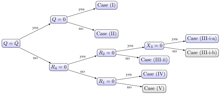
We are now ready to proceed with the classification of supersymmetric Robinson-Trautman solutions. We first divide the analysis into $Q=\bar{Q}$ or not. In the case of the real charge function ($Q=\bar{Q}$), we can consider two subclasses: the Case (I) $Q=0$ and Case (II) $Q\neq 0$. For $Q\neq\bar{Q}$, the inspection of (73c) allows us to categorize the solutions according to (III) $R_{4}=0$, (IV) $R_{1}=0$ ($R_{4}\neq 0$) and (V) $\cos(\alpha+\Theta_{1}+\Theta_{4})=0$ ($R_{1}R_{4}\neq 0$). See figure 1 for the flowchart of classification.

References

- (1) D. Klemm, M. Nozawa and M. Rabbiosi, Class. Quant. Grav. 32, no.20, 205008 (2015) doi:10.1088/0264-9381/32/20/205008 [arXiv:1506.09017 [hep-th]].
- (2) J. P. Gauntlett, N. Kim, D. Martelli and D. Waldram, “Five-branes wrapped on SLAG three-cycles and related geometry,” JHEP 0111 (2001) 018 [hep-th/0110034].
- (3) J. P. Gauntlett, D. Martelli, S. Pakis and D. Waldram, “G-structures and wrapped NS5-branes,” Commun. Math. Phys. 247 (2004) 421 [hep-th/0205050].
- (4) J. P. Gauntlett, J. B. Gutowski, C. M. Hull, S. Pakis and H. S. Reall, “All supersymmetric solutions of minimal supergravity in five- dimensions,” Class. Quant. Grav. 20 (2003) 4587 [hep-th/0209114].
- (5) J. P. Gauntlett and J. B. Gutowski, “All supersymmetric solutions of minimal gauged supergravity in five dimensions,” Phys. Rev. D 68 (2003) 105009 [Erratum-ibid. D 70 (2004) 089901] [hep-th/0304064].
- (6) J. B. Gutowski and H. S. Reall, “General supersymmetric AdS5 black holes,” JHEP 0404 (2004) 048 [hep-th/0401129].
- (7) J. B. Gutowski and W. Sabra, “General supersymmetric solutions of five-dimensional supergravity,” JHEP 0510 (2005) 039 [hep-th/0505185].
- (8) J. Bellorín, P. Meessen and T. Ortín, “All the supersymmetric solutions of , ungauged supergravity,” JHEP 0701 (2007) 020 [hep-th/0610196].
- (9) J. Bellorín and T. Ortín, “Characterization of all the supersymmetric solutions of gauged , supergravity,” JHEP 0708 (2007) 096 [arXiv:0705.2567 [hep-th]].
- (10) J. B. Gutowski, D. Martelli and H. S. Reall, “All supersymmetric solutions of minimal supergravity in six dimensions,” Class. Quant. Grav. 20 (2003) 5049 [hep-th/0306235].
- (11) J. P. Gauntlett and S. Pakis, “The geometry of Killing spinors,” JHEP 0304 (2003) 039 [hep-th/0212008].
- (12) J. P. Gauntlett, J. B. Gutowski and S. Pakis, “The geometry of null Killing spinors,” JHEP 0312 (2003) 049 [hep-th/0311112].
- (13) M. M. Caldarelli and D. Klemm, “All supersymmetric solutions of , gauged supergravity,” JHEP 0309 (2003) 019 [hep-th/0307022].
- (14) J. Bellorín and T. Ortín, “All the supersymmetric configurations of , supergravity,” Nucl. Phys. B 726 (2005) 171 [hep-th/0506056].
- (15) P. Meessen, T. Ortín and S. Vaulà, “All the timelike supersymmetric solutions of all ungauged supergravities,” JHEP 1011 (2010) 072 [arXiv:1006.0239 [hep-th]].
- (16) P. Meessen and T. Ortín, “Supersymmetric solutions to gauged sugra: the full timelike shebang,” Nucl. Phys. B 863 (2012) 65 [arXiv:1204.0493 [hep-th]].
- (17) M. Nozawa, Class. Quant. Grav. 28, 175013 (2011) doi:10.1088/0264-9381/28/17/175013 [arXiv:1011.0261 [hep-th]].
- (18) U. Gran, J. Gutowski and G. Papadopoulos, “The spinorial geometry of supersymmetric IIB backgrounds,” Class. Quant. Grav. 22 (2005) 2453 [hep-th/0501177].
- (19) U. Gran, J. Gutowski, G. Papadopoulos and D. Roest, “Systematics of IIB spinorial geometry,” Class. Quant. Grav. 23 (2006) 1617 [hep-th/0507087].
- (20) S. L. Cacciatori, M. M. Caldarelli, D. Klemm, D. S. Mansi and D. Roest, “Geometry of four-dimensional Killing spinors,” JHEP 0707 (2007) 046 [arXiv:0704.0247 [hep-th]].
- (21) J. B. Gutowski and W. A. Sabra, “Half-supersymmetric solutions in five-dimensional supergravity,” JHEP 0712 (2007) 025 [Erratum-ibid. 1004 (2010) 042] [arXiv:0706.3147 [hep-th]].
- (22) J. Grover, J. B. Gutowski and W. Sabra, “Null half-supersymmetric solutions in five-dimensional supergravity,” JHEP 0810 (2008) 103 [arXiv:0802.0231 [hep-th]].
- (23) S. L. Cacciatori, D. Klemm, D. S. Mansi and E. Zorzan, “All timelike supersymmetric solutions of , gauged supergravity coupled to abelian vector multiplets,” JHEP 0805 (2008) 097 [arXiv:0804.0009 [hep-th]].
- (24) D. Klemm and E. Zorzan, “All null supersymmetric backgrounds of , gauged supergravity coupled to abelian vector multiplets,” Class. Quant. Grav. 26 (2009) 145018 [arXiv:0902.4186 [hep-th]].
- (25) D. Klemm and E. Zorzan, “The timelike half-supersymmetric backgrounds of , supergravity with Fayet-Iliopoulos gauging,” Phys. Rev. D 82 (2010) 045012 [arXiv:1003.2974 [hep-th]].
- (26) K. -i. Maeda and M. Nozawa, “Black hole solutions in string theory,” Prog. Theor. Phys. Suppl. 189 (2011) 310 [arXiv:1104.1849 [hep-th]].
- (27) U. Gran, J. Gutowski and G. Papadopoulos, Phys. Rept. 794, 1-87 (2019) doi:10.1016/j.physrep.2018.11.005 [arXiv:1808.07879 [hep-th]].
- (28) K. P. Tod, “All metrics admitting supercovariantly constant spinors,” Phys. Lett. B 121 (1983) 241.
- (29) E. Newman and R. Penrose, J. Math. Phys. 3, 566-578 (1962) doi:10.1063/1.1724257
- (30) Z. Perjes, Phys. Rev. Lett. 27, 1668 (1971) doi:10.1103/PhysRevLett.27.1668
- (31) W. Israel and G. A. Wilson, J. Math. Phys. 13, 865-871 (1972) doi:10.1063/1.1666066
- (32) S. L. Cacciatori, M. M. Caldarelli, D. Klemm and D. S. Mansi, “More on BPS solutions of , gauged supergravity,” JHEP 0407 (2004) 061 [hep-th/0406238].
- (33) D. Klemm and M. Nozawa, Class. Quant. Grav. 32, no.18, 185012 (2015) doi:10.1088/0264-9381/32/18/185012 [arXiv:1504.02710 [hep-th]].
- (34) L. J. Romans, Nucl. Phys. B 383, 395 (1992) doi:10.1016/0550-3213(92)90684-4 [hep-th/9203018].
- (35) W. A. Sabra, Phys. Lett. B 458, 36-42 (1999) doi:10.1016/S0370-2693(99)00564-X [arXiv:hep-th/9903143 [hep-th]].
- (36) A. H. Chamseddine and W. A. Sabra, Phys. Lett. B 485, 301-307 (2000) doi:10.1016/S0370-2693(00)00652-3 [arXiv:hep-th/0003213 [hep-th]].
- (37) M. M. Caldarelli and D. Klemm, “Supersymmetry of Anti-de Sitter black holes,” Nucl. Phys. B 545 (1999) 434 [hep-th/9808097].
- (38) N. Alonso-Alberca, P. Meessen and T. Ortín, “Supersymmetry of topological Kerr-Newman-Taub-NUT-adS spacetimes,” Class. Quant. Grav. 17 (2000) 2783 [arXiv:hep-th/0003071].
- (39) P. van Nieuwenhuizen and N. P. Warner, “Integrability conditions for Killing spinors,” Commun. Math. Phys. 93 (1984) 277.
- (40) J. P. S. Lemos, Nucl. Phys. B 600, 272-284 (2001) doi:10.1016/S0550-3213(01)00064-5 [arXiv:hep-th/0011234 [hep-th]].
- (41) D. Klemm and M. Nozawa, JHEP 1305, 123 (2013) doi:10.1007/JHEP05(2013)123 [arXiv:1303.3119 [hep-th]].
- (42) J. F. Plebański and M. Demiański, “Rotating, charged, and uniformly accelerating mass in general relativity,” Annals Phys. 98 (1976) 98.
- (43) A. Gnecchi, K. Hristov, D. Klemm, C. Toldo and O. Vaughan, JHEP 01, 127 (2014) doi:10.1007/JHEP01(2014)127 [arXiv:1311.1795 [hep-th]].
- (44) M. Nozawa and T. Houri, Class. Quant. Grav. 33, no.12, 125008 (2016) doi:10.1088/0264-9381/33/12/125008 [arXiv:1510.07470 [hep-th]].
- (45) M. Nozawa, Phys. Lett. B 770, 166-173 (2017) doi:10.1016/j.physletb.2017.04.064 [arXiv:1702.05210 [hep-th]].
- (46) K. Hristov, S. Katmadas and C. Toldo, Phys. Rev. D 100, no.6, 066016 (2019) doi:10.1103/PhysRevD.100.066016 [arXiv:1907.05192 [hep-th]].
- (47) P. Ferrero, J. P. Gauntlett, J. M. P. Ipiña, D. Martelli and J. Sparks, Phys. Rev. D 104, no.4, 046007 (2021) doi:10.1103/PhysRevD.104.046007 [arXiv:2012.08530 [hep-th]].
- (48) I. Robinson and A. Trautman, Phys. Rev. Lett. 4, 431-432 (1960) doi:10.1103/PhysRevLett.4.431
- (49) I. Robinson and A. Trautman, Proc. Roy. Soc. Lond. A 265, 463-473 (1962) doi:10.1098/rspa.1962.0036
- (50) K. P. Tod, Class. Quant. Grav. 6, 1159 (1989). doi:10.1088/0264-9381/6/8/015
- (51) J. Foster, E. T. Newman, J. Math. Phys. 8, 189-194 (1967). doi:10.1063/1.1705185
- (52) B. Lukács, Z. Perjés, J. Porter and A. Sebestyén, Gen. Rel. Grav. 16, 7, 691-701 (1984). doi:10.1007/BF00767861
- (53) A. D. Rendall, Class. Quant. Grav. 5, 1339 (1988). doi:10.1088/0264-9381/5/10/012
- (54) D. Singleton, Class. Quant. Grav. 7, 1333 (1990). doi:10.1088/0264-9381/7/8/012
- (55) P. Chruściel, Commun. Math. Phys. 137, 289-313 (1991) doi:10.1007/BF02431882
- (56) P. T. Chrusciel, Proc. Roy. Soc. Lond. A 436, 299-316 (1992) doi:10.1098/rspa.1992.0019
- (57) P. T. Chrusciel and D. B. Singleton, Commun. Math. Phys. 147, 137-162 (1992) doi:10.1007/BF02099531
- (58) M. A. J. Vandyck, Class. Quant. Grav. 2, 77 (1985). doi:10.1088/0264-9381/2/1/008
- (59) M. A. J. Vandyck, Class. Quant. Grav. 4, 759 (1987). doi:10.1088/0264-9381/4/3/032
- (60) B. G. Schmidt, Gen. Rel. Grav, 20, 65 (1988). doi:10.1007/BF00759256
- (61) E. N. Glass, D. C. Robinson, J. Math. Phys. 25, 3382-3386 (1984). doi.org/10.1063/1.526107
- (62) C. Hoenselaers and W. K. Schief, J. Phys. A: Math. Gen. 25 601 (1992). doi:10.1088/0305-4470/25/3/018
- (63) C. Hoenselaers and Z. Perjes, Class. Quant. Grav. 10, 375 (1993). doi:10.1088/0264-9381/10/2/019
- (64) J. Podolský and R. Švarc, Phys. Rev. D 94, no.6, 064043 (2016) doi:10.1103/PhysRevD.94.064043 [arXiv:1608.07118 [gr-qc]].
- (65) J. Bicak and J. Podolsky, Phys. Rev. D 52, 887-895 (1995) doi:10.1103/PhysRevD.52.887
- (66) J. Bicak and J. Podolsky, Phys. Rev. D 55, 1985-1993 (1997) doi:10.1103/PhysRevD.55.1985 [arXiv:gr-qc/9901018 [gr-qc]].
- (67) G. Bernardi de Freitas and H. S. Reall, JHEP 06, 148 (2014) doi:10.1007/JHEP06(2014)148 [arXiv:1403.3537 [hep-th]].
- (68) I. Bakas and K. Skenderis, JHEP 08, 056 (2014) doi:10.1007/JHEP08(2014)056 [arXiv:1404.4824 [hep-th]].
- (69) H. Adami, A. Parvizi, M. M. Sheikh-Jabbari and V. Taghiloo, JHEP 05, 191 (2024) doi:10.1007/JHEP05(2024)191 [arXiv:2402.17658 [hep-th]].
- (70) E. T. Newman and R. Posadas, Phys. Rev. 187, 1784-1791 (1969) doi:10.1103/PhysRev.187.1784
- (71) R. W. Lind and E. T. Newman, J. Math. Phys. 15, 1103-1112 (1974) doi.org/10.1063/1.1666760
- (72) J. N. Goldberg and R. K. Sachs, Gen. Relat. Grav, 41, 2, 433-444, (2009). doi:10.1007/s10714-008-0722-5
- (73) H. Stephani, D. Kramer, M. A. H. MacCallum, C. Hoenselaers and E. Herlt, doi:10.1017/CBO9780511535185
- (74) C. Kozameh, E. T. Newman and G. Silva-Ortigoza, Class. Quant. Grav. 23, 6599-6620 (2006) doi:10.1088/0264-9381/23/23/002 [arXiv:gr-qc/0607074 [gr-qc]].
- (75) J. B. Griffiths and J. Podolsky, Cambridge University Press, 2009, ISBN 978-1-139-48116-8 doi:10.1017/CBO9780511635397
- (76) Henrici, Peter, “Applied and computational complex analysis, Volume 3: Discrete Fourier analysis, Cauchy integrals, construction of conformal maps, univalent functions,” Vol. 41. John Wiley & Sons, (1993).
- (77) A. W. C. Lun and E. W. M. Chow, [arXiv:gr-qc/9409024 [gr-qc]].
- (78) C. Kozameh, H. O. Kreiss and O. Reula, Class. Quant. Grav. 25, 025004 (2008) doi:10.1088/0264-9381/25/2/025004 [arXiv:0708.1933 [gr-qc]].
- (79) P. T. Chrusciel, [arXiv:2112.02126 [gr-qc]].
- (80) D. Z. Freedman and A. K. Das, Nucl. Phys. B 120, 221 (1977). doi:10.1016/0550-3213(77)90041-4
- (81) A. Chamblin, R. Emparan, C. V. Johnson and R. C. Myers, Phys. Rev. D 60, 064018 (1999) doi:10.1103/PhysRevD.60.064018 [arXiv:hep-th/9902170 [hep-th]].
- (82) J. P. Gauntlett, E. O Colgain and O. Varela, JHEP 02, 049 (2007) doi:10.1088/1126-6708/2007/02/049 [arXiv:hep-th/0611219 [hep-th]].
- (83) M. Nozawa and T. Shiromizu, Phys. Rev. D 89, no.2, 023011 (2014) doi:10.1103/PhysRevD.89.023011 [arXiv:1310.1663 [gr-qc]].
- (84) V. A. Kostelecky and M. J. Perry, Phys. Lett. B 371, 191-198 (1996) doi:10.1016/0370-2693(95)01607-4 [arXiv:hep-th/9512222 [hep-th]].
- (85) G. Dibitetto and D. Klemm, JHEP 12, 005 (2010) doi:10.1007/JHEP12(2010)005 [arXiv:1005.4334 [hep-th]].
- (86) M. Nozawa and T. Shiromizu, Nucl. Phys. B 887, 380-399 (2014) doi:10.1016/j.nuclphysb.2014.09.002 [arXiv:1407.3355 [hep-th]].
- (87) M. Nozawa and K. Tomoda, Class. Quant. Grav. 36, 155005 (2019) doi:10.1088/1361-6382/ab2da7 [arXiv:1902.07899 [gr-qc]].
- (88) K. Hristov, C. Toldo and S. Vandoren, JHEP 12, 014 (2011) doi:10.1007/JHEP12(2011)014 [arXiv:1110.2688 [hep-th]].
- (89) J. Podolsky, Czech. J. Phys. 52, 1-10 (2002) doi:10.1023/A:1013961411430 [arXiv:gr-qc/0202033 [gr-qc]].
- (90) O. J. C. Dias and J. P. S. Lemos, Phys. Rev. D 67, 064001 (2003) doi:10.1103/PhysRevD.67.064001 [arXiv:hep-th/0210065 [hep-th]].
- (91) B. de Wit and M. van Zalk, JHEP 10, 050 (2011) doi:10.1007/JHEP10(2011)050 [arXiv:1107.3305 [hep-th]].
- (92) N. Van den Bergh and J. Carminati, Class. Quant. Grav. 37, no.21, 215010 (2020) doi:10.1088/1361-6382/abbba3 [arXiv:2009.11516 [gr-qc]].
- (93) M. Nozawa and T. Torii, Class. Quant. Grav. 41, no.6, 065016 (2024) doi:10.1088/1361-6382/ad26ec [arXiv:2310.05460 [hep-th]].
- (94) F. Faedo, D. Klemm and M. Nozawa, JHEP 11, 045 (2015) doi:10.1007/JHEP11(2015)045 [arXiv:1505.02986 [hep-th]].
- (95) M. Nozawa, Phys. Rev. D 103, no.2, 024005 (2021) doi:10.1103/PhysRevD.103.024005 [arXiv:2010.07561 [gr-qc]].
- (96) H. Lü and J. F. Vázquez-Poritz, JHEP 12, 057 (2014) doi:10.1007/JHEP12(2014)057 [arXiv:1408.6531 [hep-th]].
- (97) M. Nozawa and T. Torii, Phys. Rev. D 107, no.6, 064064 (2023) doi:10.1103/PhysRevD.107.064064 [arXiv:2211.06517 [hep-th]].