Supervised topic models for clinical interpretability
Abstract
Supervised topic models can help clinical researchers find interpretable cooccurence patterns in count data that are relevant for diagnostics. However, standard formulations of supervised Latent Dirichlet Allocation have two problems. First, when documents have many more words than labels, the influence of the labels will be negligible. Second, due to conditional independence assumptions in the graphical model the impact of supervised labels on the learned topic-word probabilities is often minimal, leading to poor predictions on heldout data. We investigate penalized optimization methods for training sLDA that produce interpretable topic-word parameters and useful heldout predictions, using recognition networks to speed-up inference. We report preliminary results on synthetic data and on predicting successful anti-depressant medication given a patient’s diagnostic history.
1 Introduction
Abundant count data—procedures, diagnoses, meds—are produced during clinical care. An important question is how such data can assist treatment decisions. Standard pipelines usually involve some dimensionality reduction—there are over 14,000 diagnostic ICD9-CM codes alone—followed by training on the task of interest. Topic models such as latent Dirichlet allocation (LDA) (Blei, 2012) are a popular tool for such dimensionality reduction (e.g. Paul and Dredze (2014) or Ghassemi et al. (2014)). However, especially given noise and irrelevant signal in the data, this two-stage procedure may not produce the best predictions; thus many efforts have tried to incorporate observed labels into the dimensionality reduction model. The most natural extension is supervised LDA (McAuliffe and Blei, 2007), though other attempts exist (Zhu et al., 2012, Lacoste-Julien et al., 2009).
Unfortunately, a recent survey by Halpern et al. (2012) finds that many of these approaches have little benefit, if any, over standard LDA. We take inspiration from recent work (Chen et al., 2015) to develop an optimization algorithm that prioritizes document-topic embedding functions useful for heldout data and allows a penalized balance of generative and discriminative terms, overcoming problems with traditional maximum likelihood point estimation or more Bayesian approximate posterior estimation. We extend this work with recognition network that allows us to scale to a data set of over 800,000 patient encounters via an approximation to the ideal but expensive embedding required at each document.
2 Methods
We consider models for collections of documents, each drawn from the same finite vocabulary of possible word types. Each document consists of a supervised binary label (extensions to non-binary labels are straightforward) and observed word tokens , with each word token an indicator of a vocabulary type. We can compactly write as a sparse count histogram, where indicates the count of how many words of type appear in document .
2.1 Supervised LDA and Its Drawbacks
Supervised LDA (McAuliffe and Blei, 2007) is a generative model with the following log-likelihoods:
| (1) | ||||
where is the probability of topic in document , is the probability of word in topic , are coefficients for predicting label from doc-topic probabilities via logistic regression, and is the sigmoid function. Conjugate Dirichlet priors and can be easily incorporated.
For many applications, we wish to either make predictions of or inspect the topic-word probabilities directly. In these cases, point estimation is a simple and effective training goal, via the objective:
| (2) |
We include penalty weights to allow adjusting the importance of the unsupervised data term and the supervised label term. Taddy (2012) gives a coordinate ascent algorithm for the totally unsupervised objective (), using natural parameterization to obtain simple updates. Similar algorithms exist for all valid penalty weights.
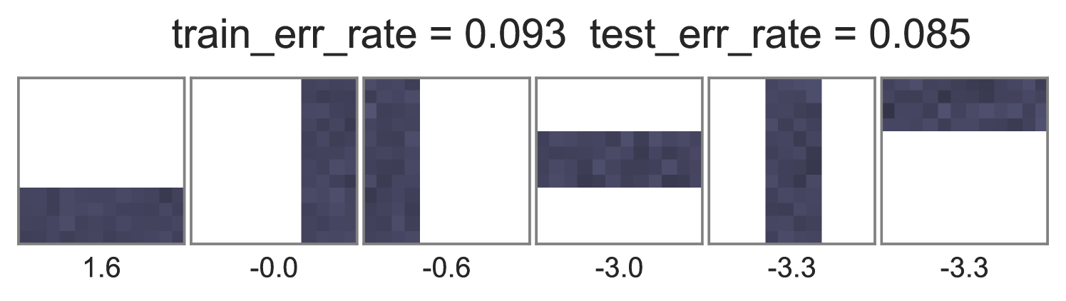
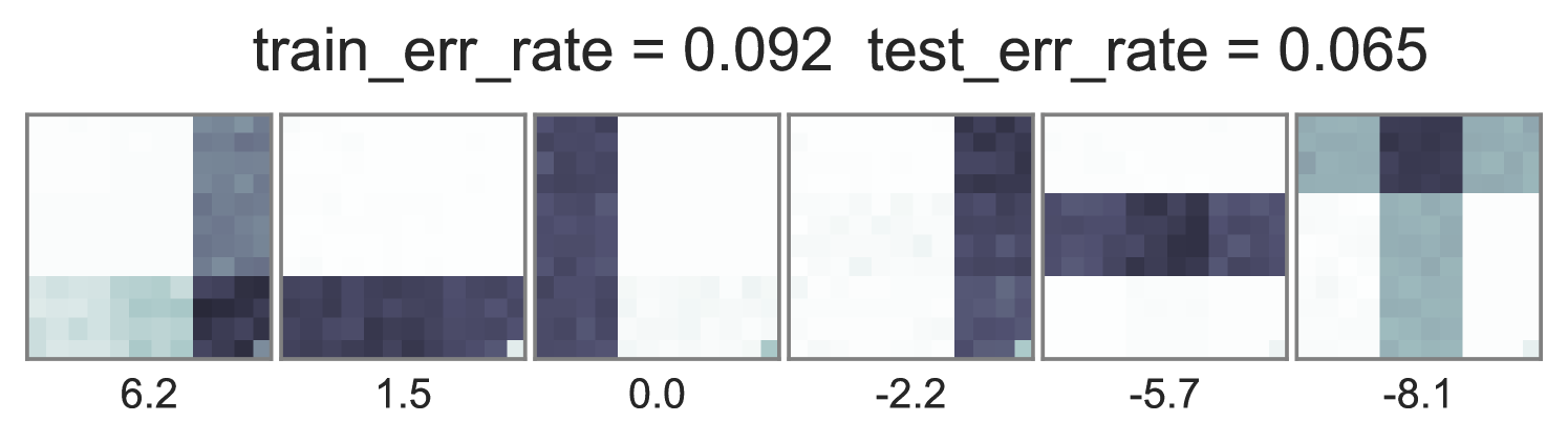
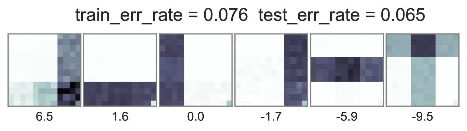
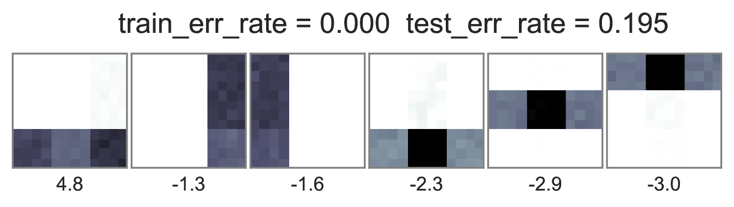
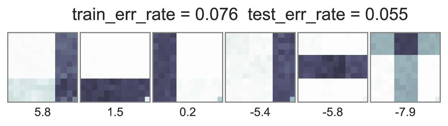
Two problems arise in practice with such training. First, the standard supervised LDA model sets . However, when contains many words but has a few binary labels, the term dominates the objective. We see in Fig. 1 that the estimated topic word parameters barely change between and under this standard training.
Second, the impact of observed labels on topic-word probabilities can be negligible. According to the model, when the document-topic probabilities are represented, the variables are conditionally independent of . At training time the may be coerced by direct updates using observed labels to make good predictions, but such quality may not be available at test-time, when must be updated using and alone. Intuitively, this problem comes from the objective treating and as “equal” observations when they are not. Our testing scenario always predicts labels from the words . Ignoring this can lead to severe overfitting, particularly when the word weight is small.
2.2 End-to-End Optimization
Introducing weights and can help address the first concern (and are equivalent to providing a threshold on prediction quality). To address the second concern, we pursue gradient-based inference of a modified version of the objective in Eq. (2) that respects the need to use the same embedding of observed words into low-dimensional in both training and test scenarios:
| (3) |
The function maps the counts and topic-word parameters to the optimal unsupervised LDA proportions . The question, of course, is how to define the function . One can estimate by solving a maximum a-posteriori (MAP) optimization problem over the space of valid dimensional probability vectors :
| (4) |
We can compute via the exponentiated gradient algorithm (Kivinen and Warmuth, 1997), as described in (Sontag and Roy, 2011). We begin with a uniform probability vector, and iteratively reweight each entry by the exponentiated gradient until convergence using fixed stepsize :
| (5) |
We can view the final result after iterations, , as a deterministic function of the input document and topic-word parameters .
End-to-end training with ideal embedding.
The procedure above does not directly lead to a way to estimate to maximize the objective in Eq. (3). Recently, Chen et al. (2015) developed backpropagation supervised LDA (BP-sLDA), which optimizes Eq. (3) under the extreme discriminative setting by pushing gradients through the exponentiated gradient updates above. We can further estimate under any valid weights with this objective. We call this “training with ideal embedding”, because the embedding is optimal under the unsupervised model.
End-to-end training with approximate embedding.
Direct optimization of the ideal embedding function , as done by Chen et al. (2015), has high implementation complexity and runtime cost. We find in practice that each document requires dozens or even hundreds of the iterations in Eq. (5) to converge reasonably. Performing such iterations at scale and back-propagating through them is possible with careful C++ implementation but will still be the computational bottleneck. Instead, we suggest an approximation: use a simpler embedding function which has been trained to approximate the ideal embedding. Initial experiments suggest a simple multi-layer perceptron (MLP) recognition network architecture with one hidden layer of size does reasonably well:
| (6) |
During training, we periodically pause our gradient descent over and update to minimize a KL-divergence loss between the approximate embedding and the ideal, expensive embedding .
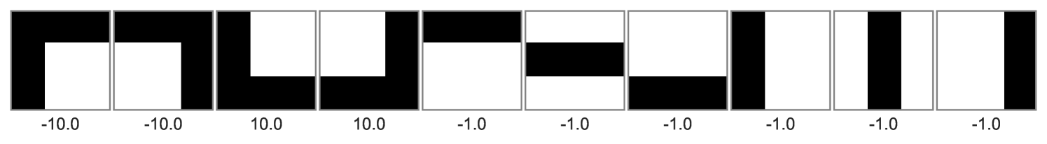
| true topics: |
|
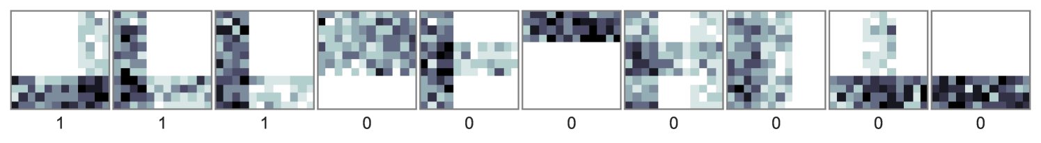
example docs: |
|
| Train with Instantiated | Train with Ideal Embedding | Train with Approx. Embedding | |
|---|---|---|---|
|
|

|
|

|
|
|
|
|
|
|
|
| N/A |
|
|
3 Case study: Toy bars data
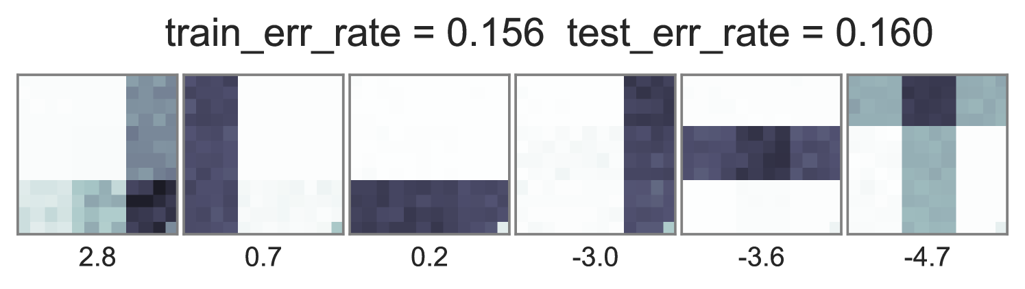
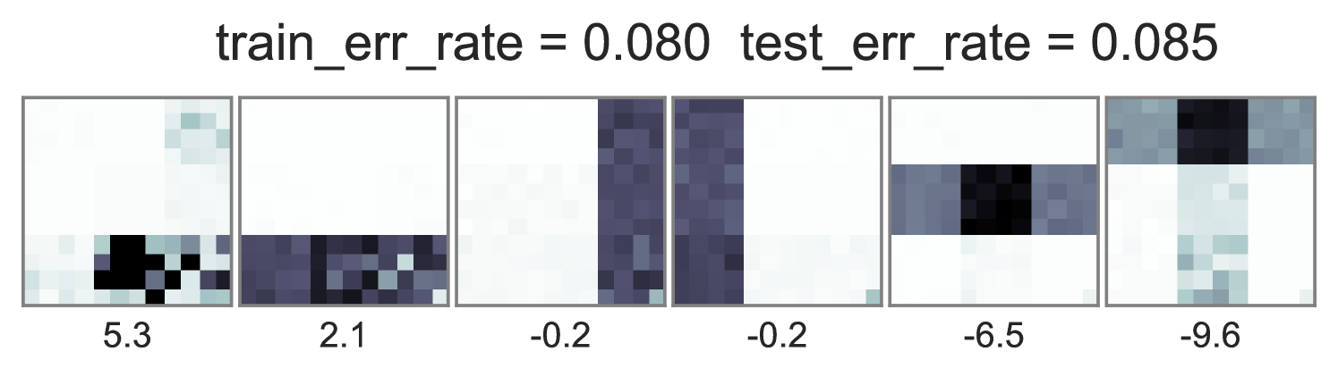
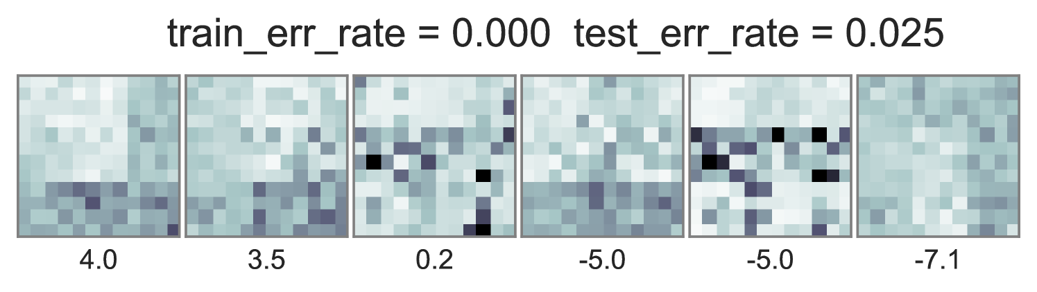
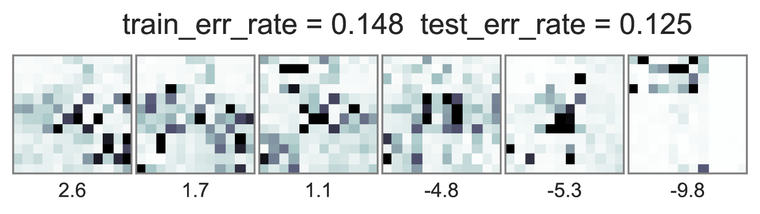
To understand how different training objectives impact both predictive performance and interpretability of topic-word parameters, we consider a version of the toy bars dataset inspired by Griffiths and Steyvers (2004), but changed so the optimal parameters are distinct for unsupervised LDA and supervised LDA objectives. Our dataset has 144 vocabulary words visualized as pixels in a square grid in Fig. 1. To generate the observed words , we use 6 true topics: 3 horizontal bars and 3 vertical bars. However, we generate label using an expanded set of 10 topics, where the extra topics are combinations of the 6 bars. Some combinations produce positive labels, but no single bar does. We train multiple initializations of each possible training objective and penalty weight setting, and show the best run of each method in Fig. 1. Our conclusions are listed below:
Standard training that instantiates can either ignore labels or overfit. Fig. 1’s first column shows two problematic behaviors with the optimization objective in Eq. (2). First, when , the topic-word parameters are basically identical whether labels are ignored () or included (). Second, when the observed data is weighted very low (), we see severe overfitting, where the learned embeddings at training time are not reproducible at test time.
Ideal end-to-end training can be more predictive but has expensive runtime. In contrast to the problems with standard training, we see in the middle column of Fig. 1 that using the ideal test-time embedding function also during training can produce much lower error rates on heldout data. Varying the data weight interpolates between interpretable topic-word parameters and good predictions. One caveat to ideal embedding is its expensiveness: Completing 100 sweeps through this 1000 document toy dataset takes about 2.5 hours using our vectorized pure Python with autograd.
Approximate end-to-end training is much cheaper and often does as well. We see in the far right column of Fig. 1 that using our proposed approximate embedding often yields similar predictive power and interpretable topic-word parameters when . Furthermore, it is about 3.6X faster to train due to avoiding the expensive embedding iterations at every document.
| approx | ideal | ideal | ideal | ideal | BoW | |
|---|---|---|---|---|---|---|
| (prevalence) DRUG | ||||||
| (0.215) citalopram | 0.65 | 0.64 | 0.63 | 0.62 | 0.61 | 0.72 |
| (0.135) fluoxetine | 0.66 | 0.64 | 0.64 | 0.63 | 0.63 | 0.76 |
| (0.133) sertraline | 0.66 | 0.66 | 0.63 | 0.63 | 0.63 | 0.75 |
| (0.119) trazodone | 0.64 | 0.66 | 0.64 | 0.61 | 0.62 | 0.65 |
| (0.115) bupropion | 0.64 | 0.64 | 0.59 | 0.56 | 0.58 | 0.71 |
| (0.070) amitriptyline | 0.77 | 0.76 | 0.77 | 0.75 | 0.75 | 0.78 |
| (0.059) venlafaxine | 0.64 | 0.62 | 0.62 | 0.61 | 0.61 | 0.73 |
| (0.059) paroxetine | 0.68 | 0.73 | 0.74 | 0.76 | 0.75 | 0.76 |
| (0.047) mirtazapine | 0.70 | 0.69 | 0.70 | 0.71 | 0.70 | 0.67 |
| (0.046) duloxetine | 0.71 | 0.69 | 0.70 | 0.69 | 0.70 | 0.74 |
| (0.041) escitalopram | 0.65 | 0.62 | 0.61 | 0.61 | 0.61 | 0.80 |
| (0.038) nortriptyline | 0.71 | 0.73 | 0.70 | 0.70 | 0.71 | 0.71 |
| (0.007) fluvoxamine | 0.70 | 0.72 | 0.74 | 0.77 | 0.76 | 0.93 |
| (0.007) imipramine | 0.40 | 0.56 | 0.50 | 0.48 | 0.48 | 0.82 |
| (0.006) desipramine | 0.47 | 0.57 | 0.54 | 0.57 | 0.54 | 0.72 |
| (0.003) nefazodone | 0.71 | 0.65 | 0.71 | 0.72 | 0.72 | 0.80 |
4 Case study: Predicting drugs to treat depression
We study a cohort of 875080 encounters from 49322 patients drawn from two large academic medical centers with at least one ICD9 diagnostic code for major depressive disorder (ICD9s 296.2x or 3x or 311, or ICD10 equivalent). Each included patient had an identified successful treatment: a prescription repeated at least 3 times in 6 months with no change.
We extracted all procedures, diagnoses, labs, and meds from the EHR (22,000 total codewords). For each encounter, we built by concatenating count histograms from the last three months and all prior history. To simplify, we reduced this to the 9621 codewords that occurred in at least 1000 distinct encounters. The prediction goal was to identify which of 16 common anti-depressants drugs would be successful for each patient. (Predicting all 25 primaries and 166 augments is future work).
Table 1 compares each method’s area-under-the-ROC-curve (AUC) with topics on a held-out set of 10% of patients. We see that our training algorithm using the ideal embedding improves its predictions over a baseline unsupervised LDA model as the weight is driven to zero. Our approximate embedding is roughly 2-6X faster, allowing a full pass through all 800K encounters in about 8 hours, yet offers competitive performance on many drug tasks except for those like desipramine or imipramine for which less than 1% of encounters have a positive label. Unfortunately, our best sLDA model is inferior to simple bag-of-words features plus a logistic regression classifier (rightmost column “BoW”), which we guess is due to local optima. To remedy this, future work can explore improved data-driven initializations.
References
- Blei (2012) D. M. Blei. Probabilistic topic models. Communications of the ACM, 55(4):77–84, 2012.
- Chen et al. (2015) J. Chen, J. He, Y. Shen, L. Xiao, X. He, J. Gao, X. Song, and L. Deng. End-to-end learning of LDA by mirror-descent back propagation over a deep architecture. In Neural Information Processing Systems, 2015.
- Ghassemi et al. (2014) M. Ghassemi, T. Naumann, F. Doshi-Velez, N. Brimmer, R. Joshi, A. Rumshisky, and P. Szolovits. Unfolding physiological state: mortality modelling in intensive care units. In Proceedings of the 20th ACM SIGKDD international conference on Knowledge discovery and data mining, pages 75–84. ACM, 2014.
- Griffiths and Steyvers (2004) T. L. Griffiths and M. Steyvers. Finding scientific topics. Proceedings of the National Academy of Sciences, 2004.
- Halpern et al. (2012) Y. Halpern, S. Horng, L. A. Nathanson, N. I. Shapiro, and D. Sontag. A comparison of dimensionality reduction techniques for unstructured clinical text. In ICML workshop on clinical data analysis, 2012.
- Kivinen and Warmuth (1997) J. Kivinen and M. K. Warmuth. Exponentiated gradient versus gradient descent for linear predictors. Information and Computation, 132(1):1–63, 1997.
- Lacoste-Julien et al. (2009) S. Lacoste-Julien, F. Sha, and M. I. Jordan. DiscLDA: Discriminative learning for dimensionality reduction and classification. In Neural Information Processing Systems, 2009.
- McAuliffe and Blei (2007) J. D. McAuliffe and D. M. Blei. Supervised topic models. In Neural Information Processing Systems, 2007.
- Paul and Dredze (2014) M. J. Paul and M. Dredze. Discovering health topics in social media using topic models. PLoS One, 9(8):e103408, 2014.
- Sontag and Roy (2011) D. Sontag and D. Roy. Complexity of inference in latent dirichlet allocation. In Neural Information Processing Systems, 2011.
- Taddy (2012) M. Taddy. On estimation and selection for topic models. In Artificial Intelligence and Statistics, 2012.
- Zhu et al. (2012) J. Zhu, A. Ahmed, and E. P. Xing. MedLDA: maximum margin supervised topic models. The Journal of Machine Learning Research, 13(1):2237–2278, 2012.