Supplemental Material: Collective motion of driven semiflexible filaments tuned by soft repulsion and stiffness

Our semiflexible filaments are modeled as discretized wormlike chains kratky49 with rigid, inextensible segments. We adopt the algorithm for constrained Brownian dynamics of bead-rod wormlike chains with anisotropic friction by Montesi et. al montesi05 . The details that follow are an overview of the algorithm introduced in their paper, with the addition of interactions and self-propulsion forces.

Filaments are represented by $N$ sites and $N-1$ segments, with fixed segment length $a$, contour length $L=(N-1)a$, and anisotropic friction, $\zeta_{\bot}=2\zeta_{\parallel}$. The position of each site $\mathbf{r}_{i}$ is updated using a midstep algorithm

where $\Delta t$ is the time step, $\mathbf{v}_{i}^{(0)}$ is the initial velocity of site $i$ at initial position $\mathbf{r}_{i}^{(0)}$, and $\mathbf{v}_{i}^{(1/2)}$ is the velocity of site $i$ recalculated at the midstep position $\mathbf{r}_{i}^{(1/2)}$, but using the same stochastic forces as in $\mathbf{v}_{i}^{(0)}$. Each site $i$ is assigned an orientation, corresponding to the orientation of the segment attaching it to site $i+1$,

The orientation of the last site of the filament is set equal to that of its only neighboring segment, so that $\mathbf{u}_{N}=\mathbf{u}_{N-1}$.

The velocity of each site is

where $\mathbf{H}_{ij}$ is an anisotropic mobility tensor, and is the mobility of site $i$ in response to a force on site $j$. The total force on site $i$ is the sum

The deterministic forces include filament bending forces, metric forces, tension forces, and external forces from interactions. $\bm{\eta}_{i}$ are the random forces contributing to the Brownian motion of the filament, and are geometrically-projected such that the forces due not break the constraints due to the fixed segment length, and are described in detail by Montesi et al. montesi05 .

The mobility tensor can be written as an inverse site friction tensor

where $\tilde{\mathbf{u}}_{i}$ is a vector tangent to site $i$, the $\otimes$ symbol denotes the outer product, and the parallel and perpendicular friction coefficients corresponding to site $i$ are $\zeta_{\parallel}^{i}$ and $\zeta_{\bot}^{i}$ respectively. The tangent vector is the average of the orientations $\mathbf{u}_{i}$ of its neighboring segments,

for $2\leq i\leq N$, and $\tilde{\mathbf{u}}_{1}=\mathbf{u}_{1}$, $\tilde{\mathbf{u}}_{N}=\mathbf{u}_{N-1}$ at the chain ends. The position update routine in Eqn. 1 can be rewritten in terms of the inverse site friction tensor as

The diffusivity of the wormlike chain is $D=k_{B}T/\zeta=k_{B}T/N\zeta^{i}$, where $\zeta^{i}$ is the local friction due to site $i$, which depends on the filament aspect ratio $L/d$ where $d$ is the diameter of the chain. In the regime of rigid, infinitely thin rods, the coefficient of friction is given by doi88 ,

where $\epsilon=1/\ln{(L/d)}$. In the finite aspect ratio case, this friction coefficient is multiplied by a geometric factor

Therefore, each site experiences a local friction given by

The bending energy of a discrete wormlike chain for $N\gg 1$ is approximated by

where $\kappa$ is the bending rigidity, which is related to the persistence length $L_{p}$ of the wormlike chain as $\kappa/k_{B}T=L_{p}$. Note that we are adopting the convention that the previous equation is true in all dimensions $d$ of wormlike chains, unlike the convention adopted by Landau and Lifshitz where $\kappa/k_{B}T=(d-1)L_{p}/2$ landau86 . This results in a Kuhn length that depends on dimensionality, $b=(d-1)L_{p}$, which is critical when analyzing the correlations of the wormlike chain for $d=2$, as discussed later.

The bending force is $\mathbf{F}^{\text{bend}}_{i}=-\partial U_{\text{bend}}/\partial\mathbf{r}_{i}$. The implementation of the bending forces coincides with metric forces, which come from a metric pseudo-potential

and $\hat{\mathbf{G}}$ is the metric tensor, which is an $(N-1)\times(N-1)$ tridiagonal matrix. $\hat{\mathbf{G}}$ has diagonal terms $d_{i}=2$ and the off-diagonal terms depend on the cosine of the angle between neighboring segments, $c_{i}=-\mathbf{u}_{i}\cdot\mathbf{u}_{i-1}$. The metric pseudo-potential is necessary for the filament conformation to have the expected statistical behavior in the flexible limit, $L_{p}\ll L$.

It was shown in the work of Pasquali et al. pasquali02 that the bending forces and metric forces could be calculated together as one force term,

where $\kappa^{\text{eff}}$ replaces the true bending rigidity $\kappa$ as an effective rigidity with a conformational dependence,

The derivative in Eqn. 14 can be evaluated from

so the two forces can be written

For an inextensible wormlike chain, the positions of $N$ sites must satisfy $N-1$ constraints $C_{\mu}$ where

for $\mu=1,\dots,N-1$. Differentiating the constraints with respect to the site positions $\mathbf{r}_{i}$ yields a vector

The geometrically projected random forces $\bm{\eta}_{i}$ must satisfy the property

so that the $3N$ dimensional vector of random forces $\bm{\eta}_{i}$ is locally tangent to the $3N-(N-1)=2N+1$ dimensional hypersurface to which the system is confined.

The geometrically projected random forces $\bm{\eta}$ are calculated from

where $\bm{\eta}^{\prime}_{i}$ are the unprojected random forces and $\hat{\eta}_{\mu}$ is the component of the $3N$ dimensional unprojected random force vector along direction $\mathbf{n}_{i\mu}$. The unprojected random forces at each timestep are

where $\bm{\xi}_{i}$ is a spatial vector whose elements are uniformly distributed random numbers between $-0.5,0.5$ montesi05 ; grassia95 .

To calculate $\hat{\eta}_{i}$, we solve the set of $N-1$ linear equations

where $\hat{\mathbf{G}}$ is the metric tensor. In matrix notation, this is equivalent to solving $\hat{\mathbf{G}}\hat{\bm{\eta}}=\mathbf{p}$ for $\hat{\bm{\eta}}$, and can be solved in $\mathcal{O}(N)$ steps using LU decomposition for tridiagonal matrices. Once the system is solved for $\hat{\eta}_{i}$, we use Eqn. 21 to solve for the geometrically projected random forces. While the deterministic forces are recalculated and applied at each half step of the simulation, the geometrically projected random forces are only calculated once per full simulation step at the initial site positions $\mathbf{r}_{i}^{(0)}$, and applied at each half step of the algorithm.

To calculate the tension $\mathcal{T}_{i}$, we require that the system constraints are constant, i.e. $\dot{C}_{\mu}=0$. This is equivalent to solving the system of linear equations

or

with diagonal and off-diagonal elements

and can be solved in a similar manner as Eqn. 23. The tension forces are then

External forces $\mathbf{F}^{\text{ext}}_{i}$ include forces from filament-filament interactions and self-propulsion forces from the driving of molecular motors. The filament-filament interaction forces are calculated from the derivative of the general exponential model potential (GEM-8)

where $r$ is the minimum distance between neighboring filament segments and $\sigma$ is the unit length used in the simulation, defined to be the diameter of a filament.

Forces from molecular motors are modeled in our simulations as a uniform force density $f_{\text{dr}}$ that is directed along the local filament segment orientations,

The assumptions of this model are that lattice defects are negligible for observing collective behavior of gliding filaments, and that motor binding and unbinding events occur at fast enough rates such that their behavior need not be explicitly included in the model. These assumptions are guided by experimental observations that filament velocities are constant in gliding assays, despite the presence of filament crossing events that certainly require a large number of unbinding and binding events liu11 .

Simulation software for the filament model is written in C++ and is publicly available online moore20 . The simulations were run on the Summit computing cluster anderson17 and parallelized using OpenMP. The simulations presented in this work required approximately $10^{6}$ CPU hours of computation, as a conservative estimate, plus additional resources for post-processing and analysis.

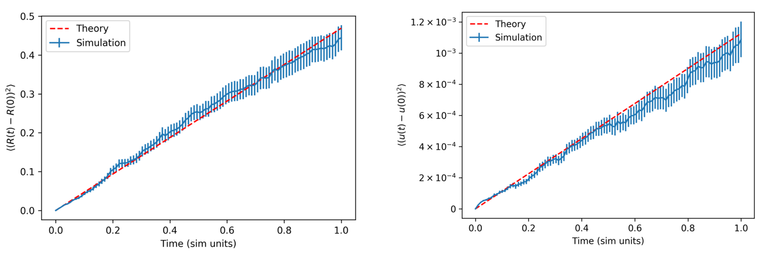
We tested the model to ensure agreement with theory for Brownian wormlike chains. Filament diffusion was validated by measuring the mean-squared displacement (MSD) and vector correlation function (VCF) for filaments in the rigid regime ($L_{p}\gg L$) and matching the expected values for slender, rigid filaments doi88 (Fig. 1).

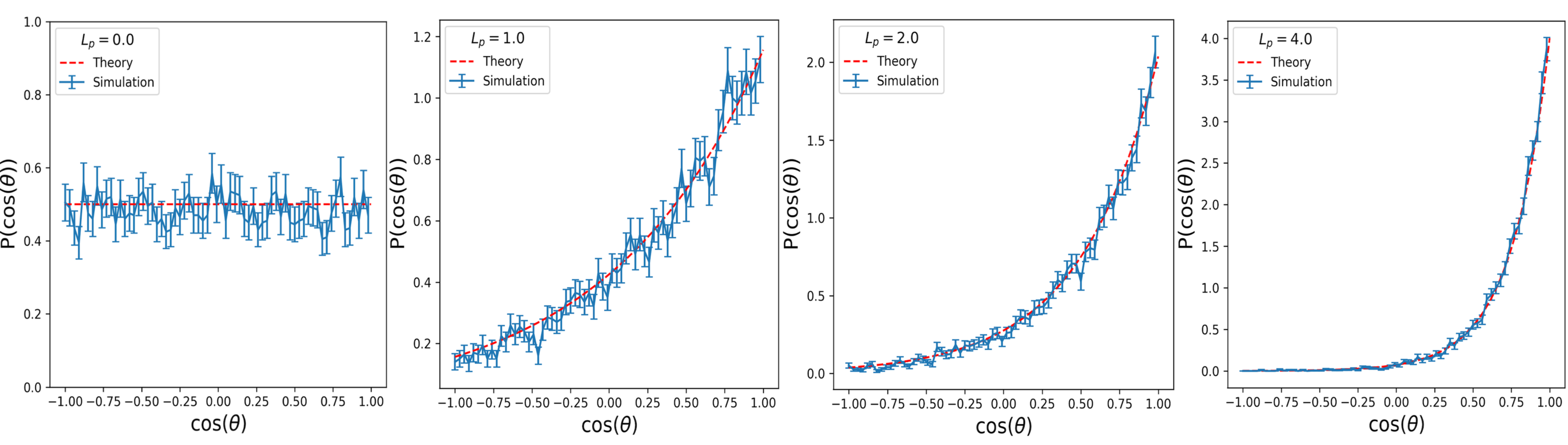
Filament bending was validated by ensuring that the conformations sampled by a filament at thermal equilibrium matched the expected statistical behavior. The distribution of angles between joining filament segments should be a Boltzmann distribution $P(\cos\theta)\propto e^{L_{p}/L\cos\theta}$. Following Montesi et al. montesi05 , we fit a histogram of filament angles from our simulation and found good agreement with the theoretical distribution (Fig. 2).

We validated the mean-square end-to-end distance $\langle R^{2}\rangle$ of the filaments in 2D. With our choice of $\kappa=L_{p}k_{B}T$ for $d=2$, $\langle R^{2}\rangle$ is given by the equation

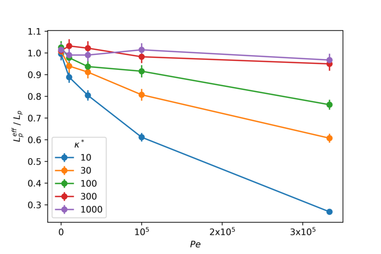
which differs from the usual result of a Kratky-Porod wormlike chain by the replacement $L_{p}\rightarrow 2L_{p}$ kratky49 . We see an apparent softening of the filament in the presence of activity, in agreement with recent reports of the same effect isele-holder15 ; singh18 ; gupta19 ; peterson20 . We plot the apparent persistence length derived from the observed $\langle R^{2}\rangle$ as a function of Péclet number in Fig. 3. The softening is appreciable at lower rigidities and vanishes for increasingly rigid filaments.

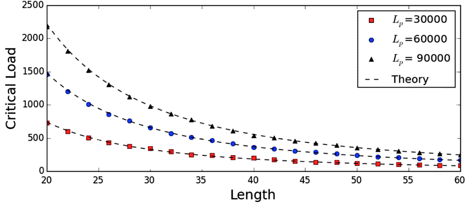
We also validated the bending model by quantifying the filament buckling behavior for rigid filaments that were placed under a load. For a rigid filament with a persistence length $L_{p}$, we expect the maximum load that an unconstrained filament can withstand before buckling to be given by Euler’s critical load for a column, $F_{cr}=\frac{\pi^{2}L_{p}k_{B}T}{L^{2}}$. To measure the critical load, we linearly increased a Hookean spring force between filament ends and recorded the force at the time when the end-to-end distance of the filament sharply deviated from the filament contour length. Varying both contour length and persistence length, we compared our measured values of the critical load to theory and found good agreement with the expected values (Fig. 4).

Key parameters of our simulation include the filament length $L$, diameter $\sigma$, persistence length $L_{p}$, driving force per unit length $f_{dr}$, repulsive energy $\epsilon$, simulation box diameter $L_{sys}$, and filament packing fraction $\phi$. In our simulations, all filaments have an aspect ratio $l=L/\sigma=60$, and the system size is $l_{sys}=L_{sys}/L=20$. In our dimensionless reduced units, $\sigma$ , $k_{B}T$, and $D$ are set to unity, where $D$ is the diffusion coefficient of a sphere with diameter $\sigma$. The driving force in reduced units is $f_{dr}=3$, $10$, and $30$, so that the corresponding Péclet numbers are $\text{Pe}=f_{dr}L^{2}/k_{B}T\approx 10^{4}$, $3.3\times 10^{4}$, $10^{5}$. When the repulsive energy $\epsilon$ in the GEM-8 potential has a value $\epsilon_{dr}=0.287\sigma f_{dr}$, the repulsive interaction between particles induces a maximum force equal to the driving force. The repulsion parameter is then rescaled to be $\tilde{\epsilon}=\epsilon/\epsilon_{dr}$ so that $\tilde{\epsilon}=l=60$ corresponds to fully impenetrable filaments in the absence of any additional forces for any given Péclet number.

The dimensionless parameters of interest when exploring the phase behavior of collective semiflexible filaments are $\tilde{\kappa}=L_{p}/L$, the rescaled energy $\tilde{\epsilon}=\epsilon/\epsilon_{dr}$, and packing fraction $\phi=A_{\text{fil}}/A_{\text{sys}}$, where $A_{\text{sys}}$ is the area of the simulation box and $A_{\text{fil}}=N(L\sigma+\pi\sigma^{2})$ is the total area occupied by $N$ spherocylindrical filaments. The timestep used in our half step integration algorithm was $\Delta t=10^{-4}\tau$, where $\tau$ is the average time for a sphere of diameter $\sigma$ to diffuse its own diameter. The active timescale is the time required for a filament to traverse its own length $\tau_{A}=l/v_{dr}=1/\zeta_{\parallel}f_{dr}$, which is $3\tau$, $\tau$, $0.33\tau$ for $\text{Pe}=10^{4},3.33\times 10^{4},10^{5}$ respectively.

Filaments in the simulation were initialized by randomly inserting filaments parallel to one axis of the simulation box in a nematic arrangement, and allowing the filaments to diffuse for $100\tau$ steps before driving the filaments. Simulations terminated once they were determined to have reached a steady state, when order parameters appeared to converge to constant values.

Six global order parameters quantify the system phase behavior, including polar order $P$, nematic order $Q$, average contact number $c$, average local polar order $p$, average spiral number $s$, and number fluctuations $\Delta N$. In addition, we quantified the dynamical flocking behavior of the system by characterizing the fraction of flocking filaments $N_{F}/N$ as well as the frequencies that filaments joined or left the flocking state, $f_{\text{NF--F}}$ and $f_{\text{F--NF}}$ respectively, which are both normalized by the number of filaments in the initial state. All order parameters are time averaged over the final 10% of the simulation.

The polar order $P$ is the normalized magnitude of the total orientation vector of all filament segments,

where $\mathbf{u}_{i}$ is the orientation of the $i^{\text{th}}$ filament segment for $N$ filaments each composed of $n$ segments. The polar order varies from $0$, where filaments have fully isotropic directional arrangement, to $1$, where all filaments are aligned in the same direction.

The nematic order is the maximum eigenvalue $Q$ of the 2D nematic order tensor

where $\mathbf{I}$ is the unit tensor. The nematic order varies from $0$, with fully isotropic directional arrangement, to $1$ where all filaments are parallel or antiparallel along the same axis.

The contact number and local polar order parameters follow previous work measuring the collective behavior of active polar particles kuan15 . The contact number is a measure of crowding in the system, and is calculated on a filament segment-wise basis,

where $s_{ij}$ is the minimum distance between segments $i$ and $j$, and with the sum excluding all intrafilament segments. The parameter $\alpha$ determines the effective cutoff for interparticle distances, which we choose to be $1/\sigma^{2}$ to only consider the contributions from nearby particles to the sum. The contact number is a purely positive quantity, ranging approximately from $0$–$10$. The average contact number is the system average of the segment contact number.

The degree of local polar ordering is determined by measuring the polar order of each segment relative to their nearest neighbors, and is weighted by the segment contact number,

where the sum again excludes intrafilament segments. The local polar order ranges from $-1$, where a segment is surrounded by filaments of opposite polarity, to $1$, where a segment is surrounded by neighboring segments with the same polarity. The average local polar order is the system average of the local polar order of all filament segments.

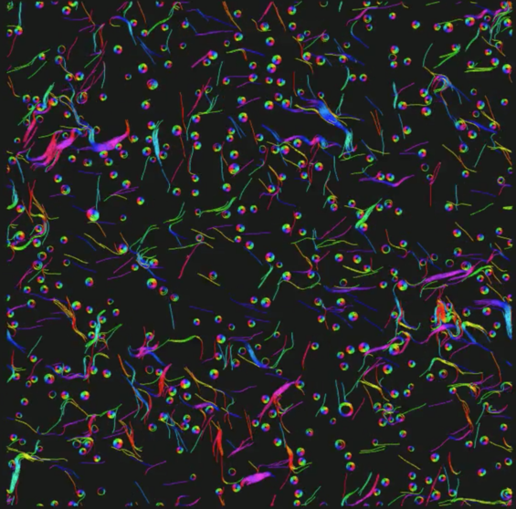
The spiral number is a measure of filament spiraling, and is calculated by measuring the angle $\theta_{i}$ swept by traversing the contour of filament $i$ from tail to head originating from the center of curvature of the filament. The average spiral number is the system average

A filament with segments that are on average oriented in a straight line will have $s\approx 0$, since the center of curvature is at a distance $\infty$ from the filament, and a filament bent into a perfect circle has $s=1$. Since filaments are not bent into perfect circles when they form a spiral, a filament spiral can be stable with a spiral number as low as $s_{i}\approx 0.8$. Filaments may also be wound very tightly and have a spiral number $s>1$.

Number fluctuations $\Delta N$ are a measure of density fluctuations in the system. The number fluctuations are determined by drawing a box of size $L_{\text{box}}<L_{\text{sys}}$ and observing the number of filaments in the box at time $t$. By time averaging the filament number within the box, one can arrive at a mean $\langle N\rangle$ and standard deviation $\Delta N$, which is a measure of the number fluctuations. By measuring $\Delta N$ and $\langle N\rangle$ for progressively larger box sizes, one can measure the scaling of the number fluctuations relative to $\langle N\rangle$, $\Delta N\propto\langle N\rangle^{\alpha}$. For equilibrium systems with particles positioned at random, the central limit theorem guarantees that $\alpha=0.5$. However, systems with collective behavior have been shown to exhibit “giant number fluctuations” (GNF), with $\alpha>0.5$. Flocking systems that have long-range order in 2D, such as the Vicsek model at low temperature, have $\alpha=0.8$ vicsek95 ; toner98 ; ginelli16 . We use the scaling of the number fluctuations $\alpha$ as an order parameter to determine the long-range ordering of the system, and find values of $\alpha$ that range between $0.5$–$0.8$ (Fig. 5).

We categorized the flocking behavior of filaments using the individual local order parameters $p_{i}$ and contact numbers $c_{i}$ for filaments. Following previous work kuan15 , we determine a filament to be flocking if $p_{i}\geq 0.5$. We also distinguish between filaments at the flock interior and exterior by labeling flocking filaments with $c_{i}\geq 0.5$ as interior flocking filaments and $c_{i}<0.5$ as exterior flocking filaments. We then tracked transitions between the three states, not flocking (NF), interior flocking (IF), and exterior flocking (EF) in order to determine the switching rates.

Only the total fraction of flocking filaments and the ratio of switching frequencies between the not-flocking state and flocking state were used as order parameters for clustering the simulation results. However, we found that saturation of the number of flocking filaments (giant flock phase) occurs when a large number of filaments are in the IF state, indicating that kinetic trapping of filaments plays an important role in stabilizing giant flocks, as observed in previous work kuan15 .

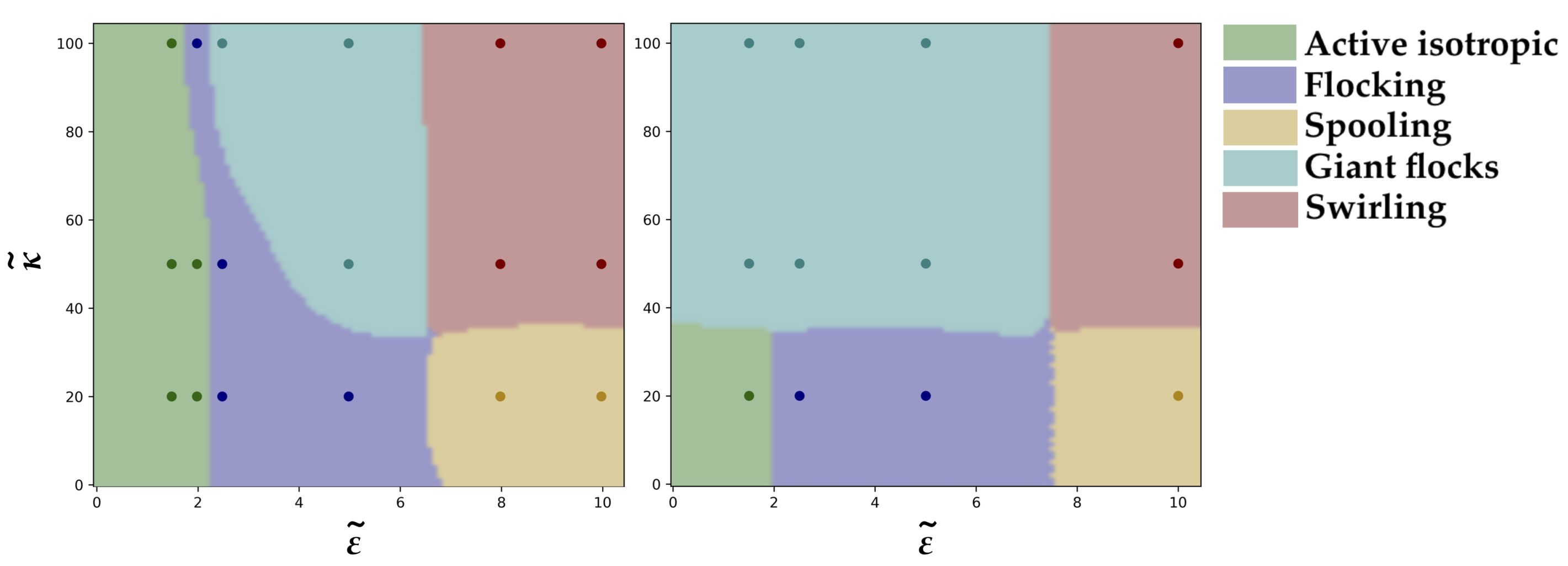
In order to label the simulation phases, simulation order parameters were grouped by Péclet number and packing fraction $\phi$ and clustered using the k-means clustering algorithm as implemented by the scikit-learn Python package scikit-learn . Initially, all order parameters values were standardized by $x-\mu/\sigma$, where $x$ is the order parameter value for a simulation, and $\mu$ and $\sigma$ are the mean and standard deviation of the same order parameter over all simulations with the same Péclet number and packing fraction. The scaled order parameters were then processed using principal component analysis, and all but the six largest components were discarded. These values were then clustered using k-means clustering for different numbers of clusters $k$, until increasing the number of clusters no longer significantly reduced the overall cost function of the algorithm. After simulations were assigned to clusters, the final simulation state behaviors were observed and labeled.

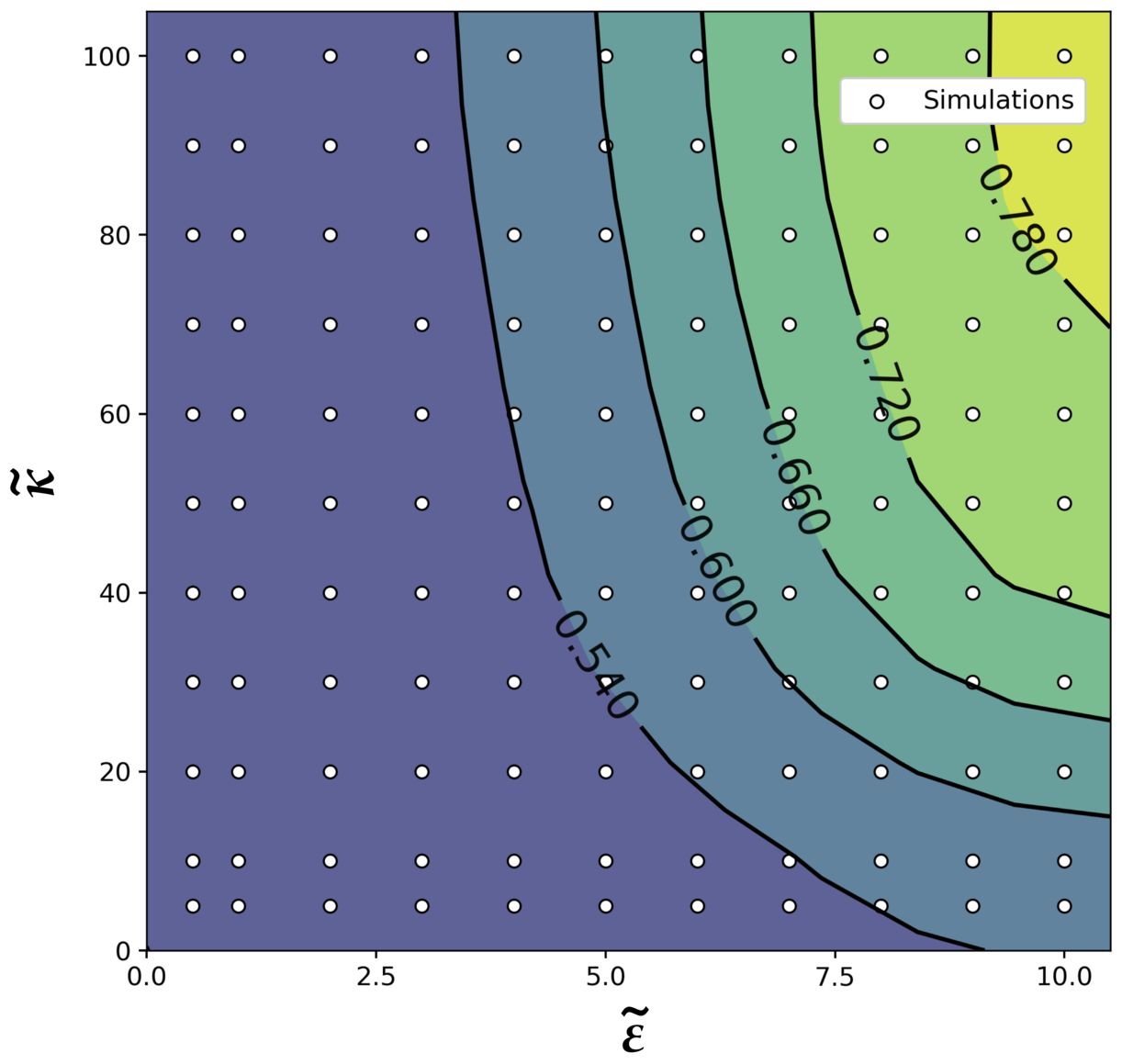
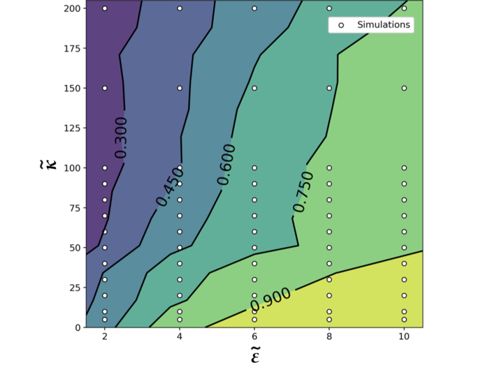
In order to determine the probability that two intersecting filaments align upon collision $P_{\text{align}}$, we simulated $10$ intersections of two filaments for $100$ initial collision angles evenly ranging between $0$ and $\pi$ in the presence of Brownian noise. We repeated this process while varying $\tilde{\kappa}$ and $\tilde{\epsilon}$ in order to determine the overall probability that two randomly-oriented filaments would align upon collision for a given filament stiffness and repulsivity (Fig. 6).

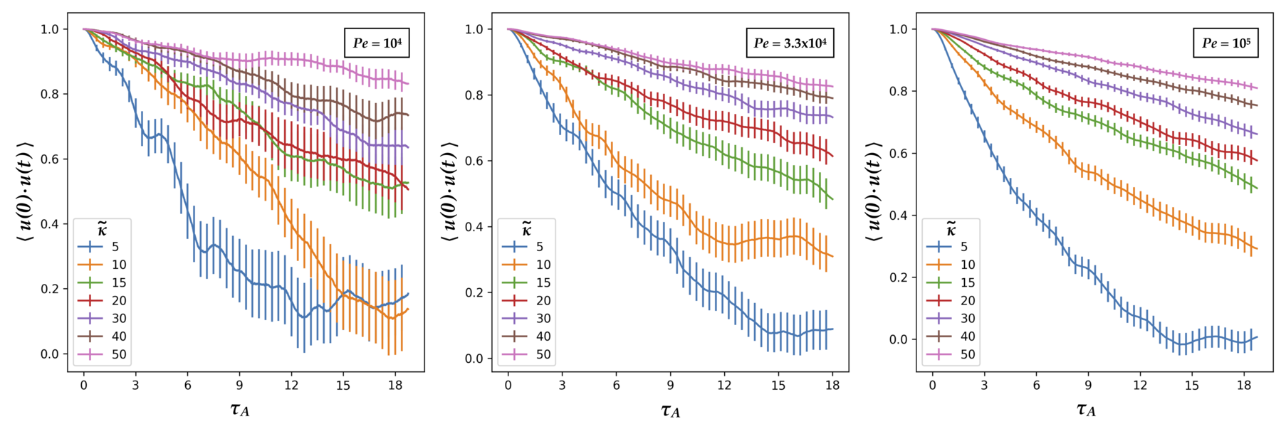
The filament orientation autocorrelation was calculated using

where $\mathbf{u}(t)$ is the orientation of the filament at time $t$, and the correlation was averaged over $N$ intervals of duration $T+t$ (Fig. 7). The filament orientation is determined by averaging over the orientation of filament segments.

Filament orientation autocorrelation lifetimes lengthen with increasing filament rigidity $\tilde{\kappa}$. For a fixed repulsion $\tilde{\epsilon}$, a longer orientation autocorrelation lifetime correlates with collective motion, which suggests that the angular persistence of filament trajectories contributes to the formation of persistent flocks and bands. For more ballistic trajectories, filaments that align can remain aligned for longer time, thus increasing the probability of aligning with more filaments along that trajectory, which may cause the accumulation of aligned filaments to form persistent flocks.

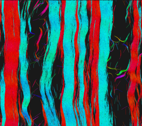
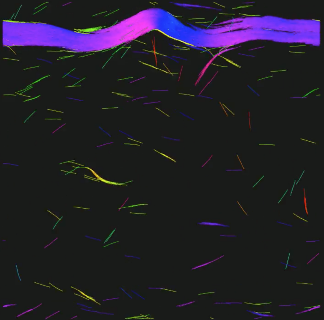
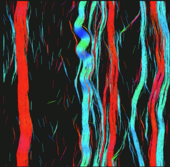
Simulations were run at $\phi=0.2$ and $0.4$, for $\tilde{\kappa}=20$, $50$, and $100$, and for values of $\tilde{\epsilon}$ ranging from $1.5$–$10$ in order to explore the parameter space at higher filament densities and search for density-dependent phase behavior. We find that the giant flock phase becomes more stable at a larger range of values of $\tilde{\epsilon}$ with increasing density (Fig. 8). At $\phi=0.4$, we found that multiple polar bands can coexist in the giant flocking phase, resulting in nematic laning, and is stable over a wide range of repulsivity. We also ran one simulation at $\phi=0.8$ at $\tilde{\epsilon}=10$ and $\tilde{\kappa}=100$, and find the giant flock/nematic laning phase to be stable at higher values of $\tilde{\epsilon}$ (Fig. 9).

We labeled the results by comparing the high density order parameter values to the results from simulations at lower filament densities. The only major inconsistency in the order parameter values between the labeled phases for low and high densities is the global polar order parameter $P$, which is high in the giant flock phase at densities $\phi\leq 0.2$, and is closer to zero at higher densities due to the presence of nematic laning bands. However, we classify nematic laning as a type of giant flocking phase, since the underlying dynamical behavior is similar.

An intrinsic curvature was added to the filament model by modifying the bending potential in Eqn. 12 to have an offset angle $\phi_{0}$,

where $\theta_{k,k-1}=\arccos{(\mathbf{u}_{k}\cdot\mathbf{u}_{k-1})}$ is the angle between site orientations $k$ and $k-1$, and $\phi_{0}=ad\phi/ds$ corresponds to the expected angle between two segments of length $a$ with a curvature per unit length $d\phi/ds$.

It can be shown that the term in the sum of Eqn. 38 can be rewritten as

where $\mathbf{R}$ is a rotation matrix that rotates the orientation vector $\mathbf{u}_{k}$ by an angle $\phi_{0}/2$,

and its inverse $\mathbf{R}^{-1}$ rotates the orientation vector $\mathbf{u}_{k-1}$ by an angle $-\phi_{0}/2$. The combined bending and metric forces from Eqn. 14 with intrinsic curvature are therefore

which can be expanded in the same way as Eqn. 17.

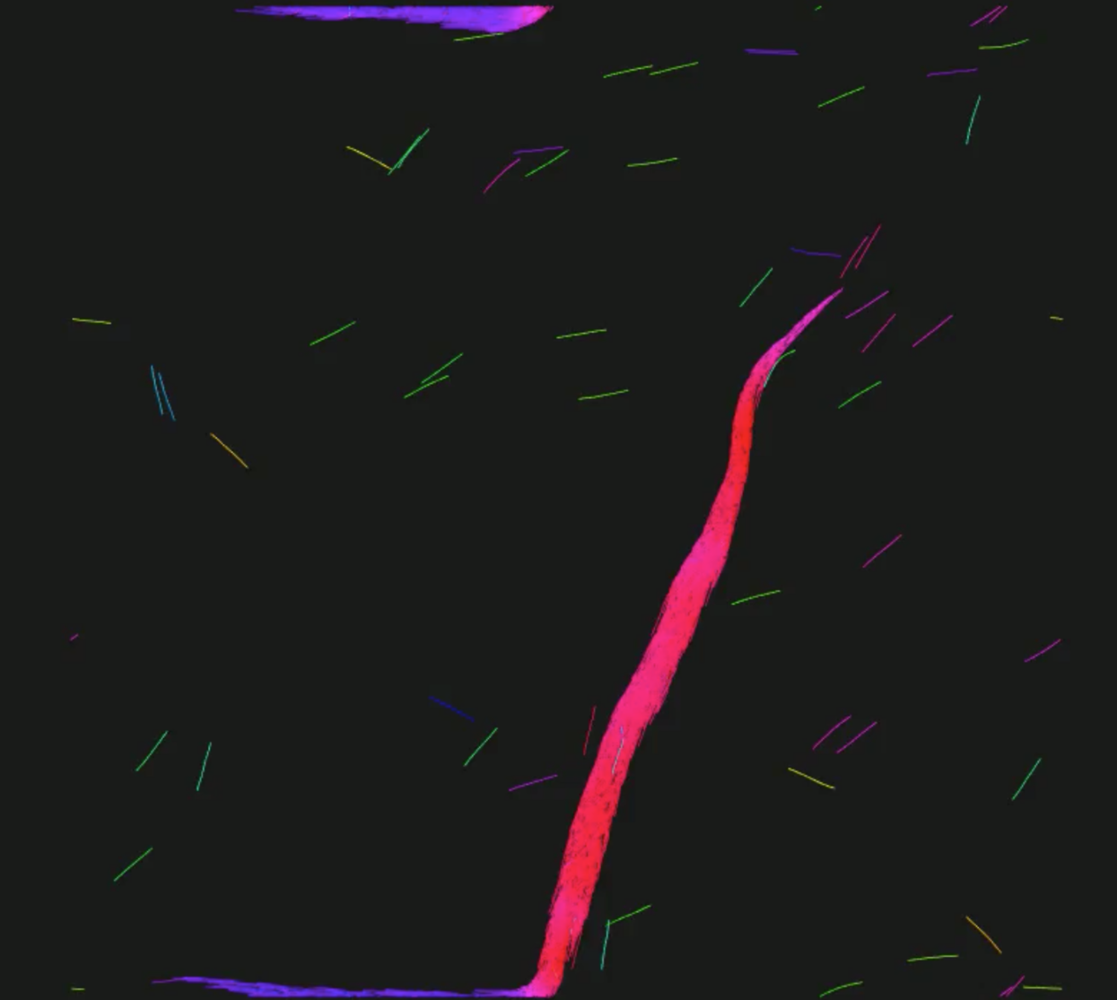
We ran a simulation with intrinsic curvature $d\phi/ds=0.02$ radians/$\sigma$, with packing fraction $\phi=0.3$, filament length $l=37$, system box length $l_{sys}=6.67l$, rigidity $\tilde{\kappa}=100$, and repulsion $\tilde{\epsilon}=5$ (Fig. 17). The filaments coalesce into a single polar band, which then buckles and reassembles at an angle rotated in the direction of filament curvature. This buckling and rotation behavior continues for the length of the simulation. The rotation of the polar order vector has been observed in filament gliding assay experiments and simulations of bead-spring filament models with intrinsic curvature kim18 .

References

- [1] O. Kratky and G. Porod. Röntgenuntersuchung gelöster fadenmoleküle. Recueil des Travaux Chimiques des Pays-Bas, 68(12):1106–1122, 1949.
- [2] Alberto Montesi, David C. Morse, and Matteo Pasquali. Brownian dynamics algorithm for bead-rod semiflexible chain with anisotropic friction. The Journal of Chemical Physics, 122(8):084903, February 2005.
- [3] Masao Doi and S. F. Edwards. The Theory of Polymer Dynamics. Clarendon Press, 1988.
- [4] L.D. Landau, E.M. Lifshitz, A.M. Kosevich, J.B. Sykes, L.P. Pitaevskii, and W.H. Reid. Theory of elasticity: Volume 7. Course of theoretical physics. Elsevier Science, 1986. Citation Key: landau1986theory tex.lccn: 86002450.
- [5] Matteo Pasquali and David C. Morse. An efficient algorithm for metric correction forces in simulations of linear polymers with constrained bond lengths. The Journal of Chemical Physics, 116(5):1834–1838, February 2002.
- [6] P. S. Grassia, E. J. Hinch, and L. C. Nitsche. Computer simulations of Brownian motion of complex systems. Journal of Fluid Mechanics, 282:373–403, January 1995.
- [7] Lynn Liu, Erkan Tüzel, and Jennifer L Ross. Loop formation of microtubules during gliding at high density. Journal of Physics: Condensed Matter, 23(37):374104, September 2011.
- [8] Jeffrey M. Moore. Simcore v0.2.2. Zenodo, May 2020.
- [9] Jonathon Anderson, Patrick J. Burns, Daniel Milroy, Peter Ruprecht, Thomas Hauser, and Howard Jay Siegel. Deploying RMACC Summit: An HPC Resource for the Rocky Mountain Region. In Proceedings of the Practice and Experience in Advanced Research Computing 2017 on Sustainability, Success and Impact, PEARC17, pages 8:1–8:7, New Orleans, LA, USA, 2017. ACM.
- [10] Rolf E. Isele-Holder, Jens Elgeti, and Gerhard Gompper. Self-propelled worm-like filaments: Spontaneous spiral formation, structure, and dynamics. Soft Matter, 11(36):7181–7190, 2015.
- [11] Shalabh K. Anand and Sunil P. Singh. Structure and dynamics of a self-propelled semiflexible filament. Physical Review E, 98(4):042501, Oct 2018.
- [12] Nisha Gupta, Abhishek Chaudhuri, and Debasish Chaudhuri. Morphological and dynamical properties of semiflexible filaments driven by molecular motors. Physical Review E, 99(4):042405, Apr 2019.
- [13] Matthew S. E. Peterson, Michael F. Hagan, and Aparna Baskaran. Statistical properties of a tangentially driven active filament. Journal of Statistical Mechanics: Theory and Experiment, 2020(1):013216, Jan 2020.
- [14] Hui-Shun Kuan, Robert Blackwell, Loren E. Hough, Matthew A. Glaser, and M. D. Betterton. Hysteresis, reentrance, and glassy dynamics in systems of self-propelled rods. Physical Review E, 92(6), December 2015.
- [15] Tamás Vicsek, András Czirók, Eshel Ben-Jacob, Inon Cohen, and Ofer Shochet. Novel Type of Phase Transition in a System of Self-Driven Particles. Physical Review Letters, 75(6):1226–1229, August 1995.
- [16] John Toner and Yuhai Tu. Flocks, herds, and schools: A quantitative theory of flocking. Physical Review E, 58(4):4828–4858, Oct 1998.
- [17] Francesco Ginelli. The physics of the vicsek model. The European Physical Journal Special Topics, 225(11):2099–2117, Nov 2016.
- [18] F. Pedregosa, G. Varoquaux, A. Gramfort, V. Michel, B. Thirion, O. Grisel, M. Blondel, P. Prettenhofer, R. Weiss, V. Dubourg, J. Vanderplas, A. Passos, D. Cournapeau, M. Brucher, M. Perrot, and E. Duchesnay. Scikit-learn: Machine learning in Python. Journal of Machine Learning Research, 12:2825–2830, 2011.
- [19] Kyongwan Kim, Natsuhiko Yoshinaga, Sanjib Bhattacharyya, Hikaru Nakazawa, Mitsuo Umetsu, and Winfried Teizer. Large-scale chirality in an active layer of microtubules and kinesin motor proteins. Soft Matter, 14(17):3221–3231, 2018.