Supplemental Material for
An Eulerian nonlinear elastic model for compressible and fluidic tissue with radially symmetric growth
I Dynamics with Tissue Rearrangement
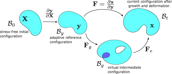
We consider that the adaptive reference configuration relaxes from the initial reference configuration to the current deformed configuration ; see Fig. S1. The relaxed reference coordinate is described by the adaptive reference map , whose dynamics is given by
| (1) |
where , is the rotational part of the deformation gradient , and is the rate of rearrangement that measures how fast the reference configuration of the tissue adapts to the current configuration. From the polar decomposition of , where is the symmetric positive-definite stretch tensor in the material coordinate, can be uniquely defined as the local rotation (orthogonal transformation ) that transforms differential elements from the tangent space in the material (curvilinear) coordinate into the tangent space in the current (curvilinear) coordinate. The combination is needed to ensure frame invariance of the tensorial evolution equations below under the rotation .
With , the adaptive reference configuration is a new configuration with respect to which we can define the effective deformation gradient . The dynamics of and its determinant is consequently affected by . Following similar derivation process in main text with the dynamics of adaptive reference map Eq. (1), we can get the dynamics of the relaxed deformation gradient
| (2) |
Notice that this equation is invariant under the rotation because , , and , where we have omitted the for simplicity. The first term with demonstrates the adaption of the deformation gradient weighted by the local Biot strain tensor . The second term shows the effect from the rotation on the dynamics of .
Then the dynamics of relaxed geometric volume variation tracked by the adaptive reference map is :
| (3) |
We assume that tissue rearrangement does not interfere the dynamics of tissue density
| (4) |
Combining the relation with eqs. 4 and 3, we obtain the dynamics of with rearrangement
| (5) |
Assuming that the growth stretch tensor is still isotropic with tissue rearrangement, the elastic deformation tensor is . Thus, the dynamics of the elastic deformation tensor is
| (6) |
The second term contributes to an anisotropic effect on the update of where is traceless. Then the dynamics of the elastic volume variation is
| (7) |
One can check that eqs. 3, 4, 5, 6 and 7 are all invariant under the rotation .
Considering the total strain energy , the rate of change of total strain energy is given by the dynamics eqs. 6 and 7
| (8) |
where the stress is given by the constitutive law
| (9) |
where and . The stress can be decomposed as , the sum of the deviatoric part (proportional to ) and the isotropic part (proportional to ). The first integral in eq. 8 represents the energy change due to active growth. The second and the third integrals represent the energy change due to the rearrangement rate . Notice is replaced by since and both vanish. Using eq. 9, one can check that is nonnegative and only vanish when is isotropic or . This means that the second integral with dissipates the stored strain energy only when there are both shear stress and shear deformation. Thus, the adaptive reference map results in physically intuitive properties in the dynamics of the total strain energy in terms related to the Biot strain . However, the last term involving is not straightforward to interpret geometrically or physically. Thus, we limit our attention to symmetric cases in this work where .
II Growth of Compressible Tissue in a 2D Disc
We have also studied the growth of tissue in a 2D disc with fixed height (where there is no deformation in the direction of its thickness). As in Sec. 5 in the main text, we first give the analytic equilibrium solutions for the linearized system. Then we show some numerical simulation results for the nonlinear system.
II.1 Mechanical Equilibrium in a 2D Disc
Writing the linearized system in the approximation of small deformation in the polar coordinates , we obtain
subject to deformation-free initial conditions and free moving boundary conditions
When the growth rate is partially positive and partially negative within the tissue, there exists an equilibrium tissue size such that
| (10) |
We can also obtain the solutions in mechanical equilibrium:
| (11) |
Similar as in the 3D case, the stresses can be dissipated with large and the variation in (and also tissue density ) is modulated by relative compressibility and tissue fluidity relative to growth .
II.2 Nonlinear Simulations
We perform simulations for the nonlinear system of tissue in a 2D disc
| (12) |
subject to the deformation-free initial condition and free moving boundary conditions
| (13) |
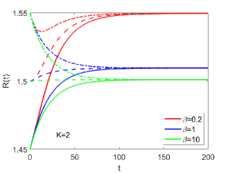
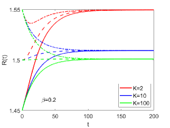
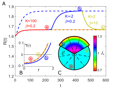
Nonlinear Effect on Equilibrium Tumor Size. We first simulate the growth of a tissue disc with prescribed growth rate (Fig. S2 B) and initial radius . The simulation results for the evolution of for different and are shown in Fig. S2 A. The inverse of density (with ) in equilibrium for different and is shown in Fig. S2 C by each sector. The evolution of with different initial sizes is shown in Fig. S3. The equilibrium size is independent on the initial size and only dependent on the tissue properties and .
The equilibrium tissue size for tissue disc satisfies the condition
| (14) |
where for the prescribed growth rate and for the growth rate coupled with chemical growth factor within the tissue disc of size . This condition demonstrates the coupling of tissue size growth with tissue mechanics.
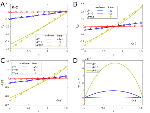
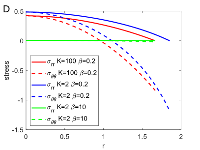
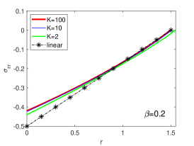
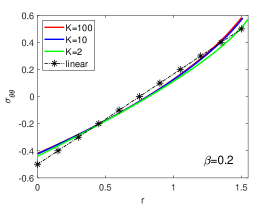
Regulation of Mechanical Stress and Tissue Density. The mechanical states including stresses , and elastic volume variation in equilibrium for different are shown in Fig. S4. They can be dissipated by fast rearrangement (large ), just as in 3D case. In particular, the incompressibility condition is achieved for (Fig. S4 D), as predicted in linear solutions. The stresses are scarcely altered by the change of , as shown in Fig. S5.
Growth Rate Coupled with Chemical Signals. We then simulate the growth of a tissue disc when the growth rate is coupled with the concentration of growth factor
| (15) |
where and are the local rates of cell proliferation and apoptosis, respectively. The concentration of growth factor within a tissue disc of size follows the reaction-diffusion process
| (16) |
Assuming , we can obtain the quasi-steady-state solution of eq. 16 for tissue radius at each time point:
| (17) |
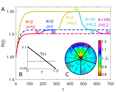
where is the modified Bessel function of first kind. We perform simulation for the growth of a tissue disc with . The evolution of for different and is shown in Fig. S6 A. The growth rate in equilibria is shown in Fig. S6 B and the elastic volume variation in equilibria is shown in Fig. S6 C. The stresses can be dissipated by large and can be moderately reduced by large , as shown in Fig. S6 D.