Supplemental Material:
Learning to Look around Objects for Top-View Representations of Outdoor Scenes
The supplemental material contains the following items:
-
•
Section 1: Additional experiments and details of the proposed hallucination models for semantic segmentation and depth prediction.
-
•
Section 2: Extended ablation study of the proposed refinement module.
-
•
Section 3: Additional qualitative results of the semantic bird’s eye view representation.
-
•
Section 4: Evaluation of semantic segmentation (and depth prediction) of foreground pixels.
1 Semantic and depth hallucination
Hallucinating the semantics and depth behind foreground objects is an important part of the proposed BEV mapping. The main paper shows two experiments for hallucination on the KITTI-Anon data set. Here, we provide an ablation study of several other aspects of the hallucination-CNN on two data sets.
First, we investigate the random box sampling strategy used for training the hallucination networks, see Section 3.1 and Figure 2(b) in the main paper. We name each sampling strategy based on four properties as “geometry - background class - object size - object count”, where each property can take the following values:
-
•
“geometry” is either “none” or “perspective (persp.)”. Perspective means that we apply a transformation to bounding boxes in order to mimic depth, \eg, objects further away become smaller. “None” means that we do not change box sizes based on any prior.
-
•
“background class” is also a prior about where bounding boxes are placed. For “road”, we only put boxes at positions where they significantly overlap with road pixels. For “bg”, significant overlap with any background class is required.
-
•
“object size” is the typical object height closest to the camera, \ie, bottom of the image in the 2D image. Note that object size is changed based on the y-axis location if the “perspective” option is used.
-
•
“object count” is the number of bounding boxes sampled per image.
In general, we can see from Table 1 that placing more or bigger bounding boxes on images during the training process is beneficial, particularly for the hidden pixels which we are most interested in. For instance, putting artificial boxes only on road pixels “persp-road-150-3”, making the boxes small “persp-bg-50-5” or only sampling a single box “persp-bg-100-1” clearly deteriorates the performance of both semantic segmentation and depth prediction for hidden pixels.
Since the hallucination CNN is jointly trained for semantic segmentation and depth prediction, we also investigate the impact of joint training of the two related tasks. We balance the loss functions for segmentation and depth prediction via , where . We can see from Table 2 that the two tasks typically help each other, \ie, a value of not at the two ends of the spectrum gives the best results. The only exception is semantic segmentation of visible pixels on the Cityscapes data set. For hidden pixels, the benefits of jointly training for both tasks can be seen on all data sets and is more pronounced than for visible pixels.
| \topruleDataset | Method | random-boxes | human-gt | ||||||||
|---|---|---|---|---|---|---|---|---|---|---|---|
| visible | hidden | visible | hidden | ||||||||
| iou | RMSE | acc | ard | iou | RMSE | acc | ard | iou | iou | ||
| \topruleKITTI- | none-bg-150-3 | 76.68 | 3.846 | 89.17 | .0923 | 64.63 | 5.360 | 74.43 | .1413 | 81.12 | 60.06 |
| Anon | persp-bg-150-3 | 75.37 | 4.510 | 88.39 | .0938 | 61.06 | 7.544 | 63.54 | .1748 | 80.21 | 60.19 |
| persp-road-150-3 | 75.03 | 4.192 | 87.89 | .0964 | 49.18 | 7.848 | 61.09 | .1890 | 80.19 | 53.18 | |
| persp-bg-50-5 | 75.94 | 4.081 | 88.34 | .0943 | 53.01 | 8.375 | 57.83 | .1979 | 80.20 | 57.50 | |
| persp-bg-100-1 | 76.09 | 4.066 | 88.19 | .0943 | 57.27 | 8.658 | 58.17 | .1959 | 80.41 | 58.11 | |
| persp-bg-100-10 | 75.80 | 4.127 | 87.63 | .0963 | 59.22 | 8.177 | 60.72 | .1864 | 79.91 | 61.92 | |
| \midruleKITTI- | none-bg-150-3 | 70.95 | 2.411 | 91.65 | .0897 | 59.38 | 1.886 | 96.76 | 0.063 | 88.70 | 65.36 |
| Ros | persp-bg-150-3 | 70.82 | 2.298 | 92.44 | .0843 | 61.90 | 1.715 | 97.15 | 0.060 | 88.22 | 61.68 |
| persp-road-150-3 | 69.14 | 2.394 | 91.65 | .0866 | 47.13 | 2.138 | 93.61 | 0.079 | 86.39 | 37.55 | |
| persp-bg-50-5 | 70.68 | 2.356 | 91.95 | .0858 | 51.92 | 2.389 | 92.23 | 0.079 | 88.08 | 53.66 | |
| persp-bg-100-1 | 70.78 | 2.295 | 92.32 | .0841 | 54.80 | 1.999 | 95.67 | 0.065 | 88.00 | 53.38 | |
| persp-bg-100-10 | 70.39 | 2.283 | 92.41 | .0837 | 61.64 | 1.698 | 97.26 | 0.056 | 87.84 | 57.69 | |
| \bottomrule | |||||||||||
| \topruleDataset | Method | random-boxes | human-gt | ||||||||
|---|---|---|---|---|---|---|---|---|---|---|---|
| visible | hidden | visible | hidden | ||||||||
| iou | RMSE | acc | ard | iou | RMSE | acc | ard | iou | iou | ||
| \topruleKITTI- | 0.00 | 72.92 | - | - | - | 62.48 | - | - | - | 79.45 | 59.78 |
| Anon | 0.25 | 75.17 | 4.105 | 87.64 | .1000 | 63.70 | 5.905 | 70.79 | .1577 | 80.24 | 60.26 |
| 0.50 | 76.20 | 3.832 | 89.44 | .0909 | 64.41 | 5.503 | 74.31 | .1446 | 80.85 | 59.39 | |
| 0.75 | 75.29 | 3.778 | 90.17 | .0873 | 63.33 | 5.334 | 76.02 | .1380 | 80.72 | 59.94 | |
| 1.00 | - | 3.921 | 88.79 | .0954 | - | 5.428 | 74.73 | .1452 | - | - | |
| \midruleKITTI- | 0.00 | 69.29 | - | - | - | 57.25 | - | - | - | 87.93 | 53.29 |
| Ros | 0.25 | 70.05 | 2.496 | 91.05 | .0918 | 60.95 | 1.940 | 95.78 | .0670 | 87.59 | 56.92 |
| 0.50 | 71.26 | 2.278 | 92.84 | .0816 | 59.54 | 1.906 | 96.58 | .0606 | 88.05 | 54.90 | |
| 0.75 | 71.39 | 2.179 | 93.58 | .0769 | 59.89 | 1.729 | 97.24 | .0570 | 88.71 | 53.77 | |
| 1.00 | - | 2.649 | 91.16 | .0896 | - | 2.166 | 94.65 | .0732 | - | - | |
| \midruleCity- | 0.00 | 71.14 | - | - | - | 59.80 | - | - | - | 74.00 | 60.27 |
| scapes | 0.25 | 70.62 | 12.810 | 84.57 | .1325 | 60.26 | 8.290 | 85.39 | .123 | 73.72 | 60.57 |
| 0.50 | 69.75 | 12.813 | 86.27 | .1234 | 58.80 | 8.226 | 86.83 | .116 | 73.49 | 61.24 | |
| 0.75 | 68.19 | 12.787 | 87.03 | .1206 | 55.69 | 8.187 | 87.24 | .112 | 72.85 | 60.89 | |
| 1.00 | - | 12.796 | 84.63 | .1333 | - | 7.848 | 85.18 | .127 | - | - | |
| \bottomrule | |||||||||||
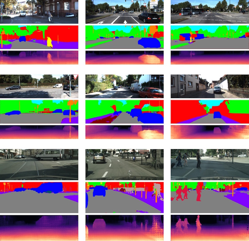
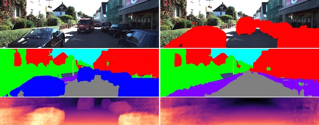
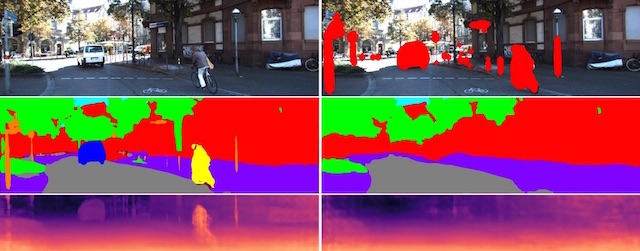
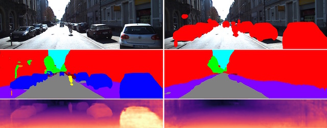
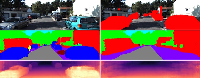
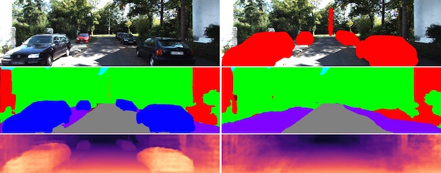
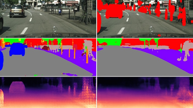
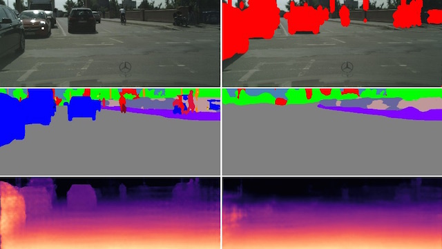
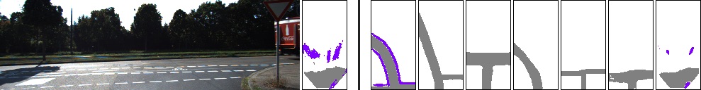
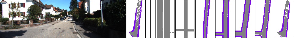
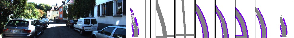
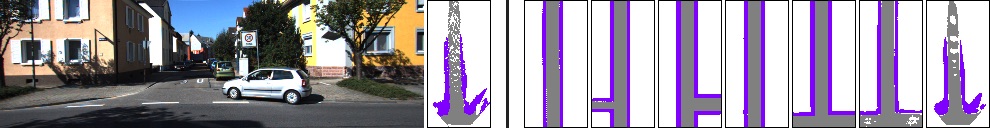
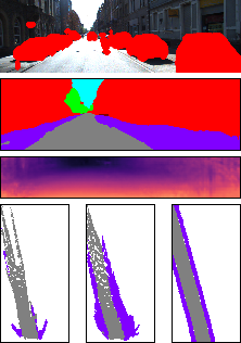
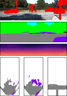
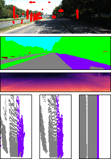
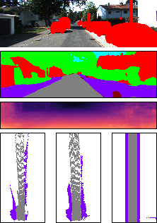
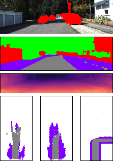
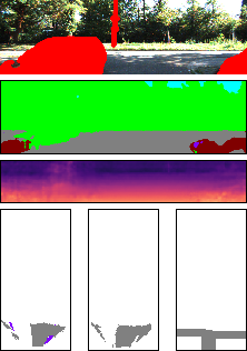
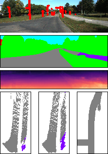
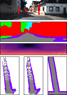
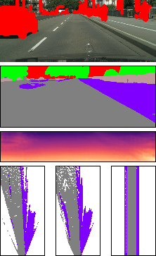
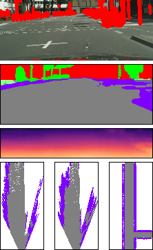
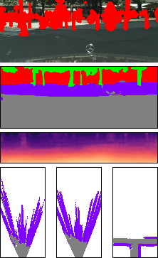
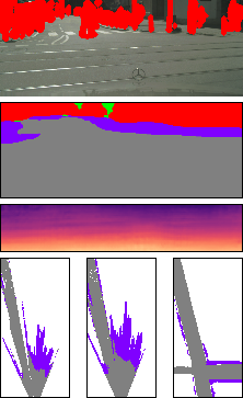
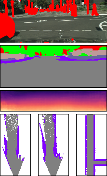
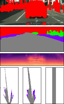
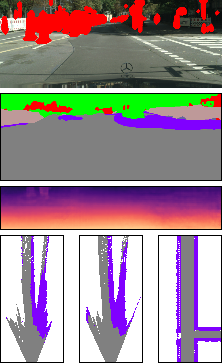
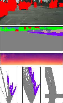
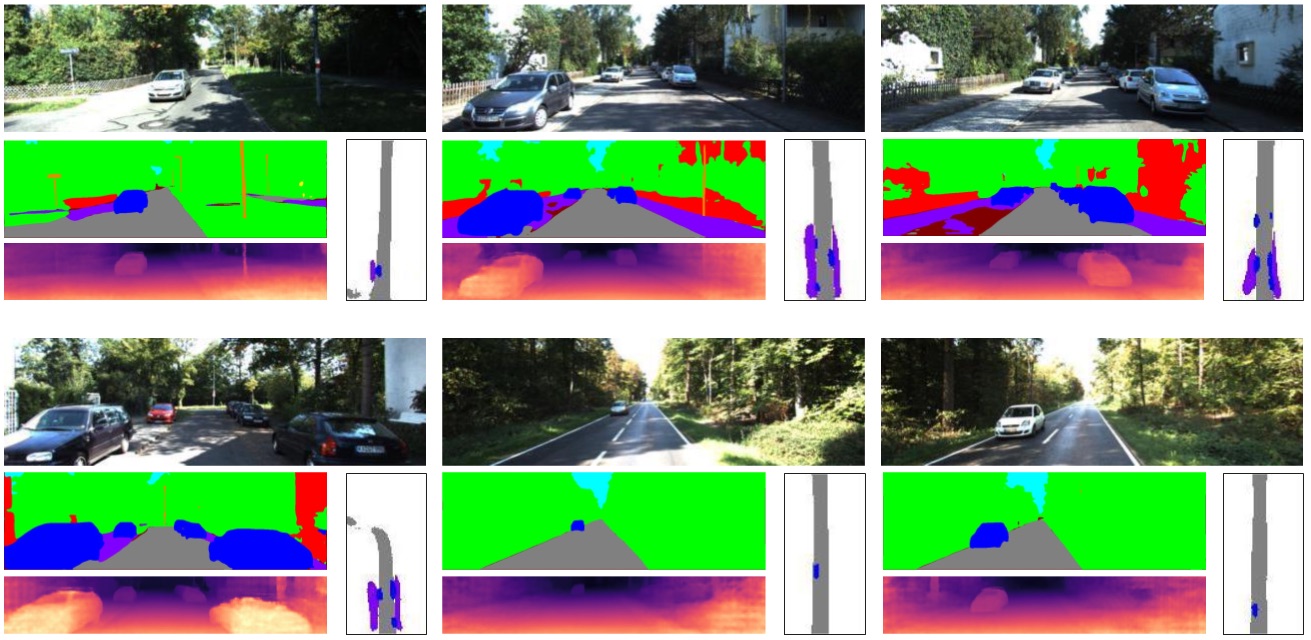
In Figure 1 we present additional qualitative results of hallucinating semantics and depth, which are contrasted with the corresponding standard foreground semantic segmentation and depth prediction. One can clearly see the prior knowledge learned by the hallucination CNN.
2 Additional results of the refinement module
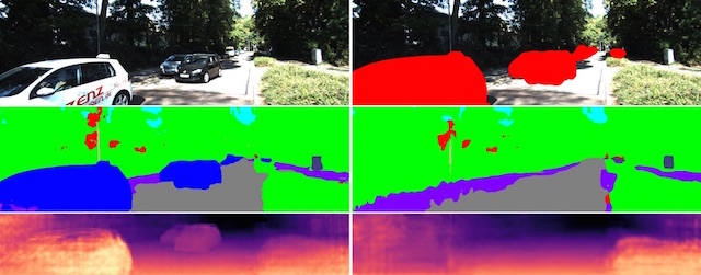
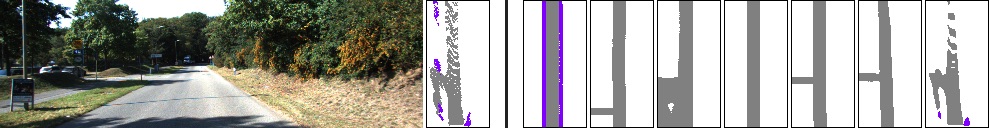
In this section, we show additional results of the impact of the trade-off between the adversarial loss (on simulated data) and the reconstruction loss (with the initial BEV map or OSM data if available). The main paper contains one example (in Figure 7). Here, we provide more examples in Figure 2. It is clearly evident from the figure that the reconstruction loss needs to be properly balanced with the adversarial loss. No reconstruction loss obviously leads to generating scene layouts that don’t match the actual image evidence. On the other hand, putting too much weight on the reconstruction loss leads the refinement module to learning the identity function without improving upon its input.
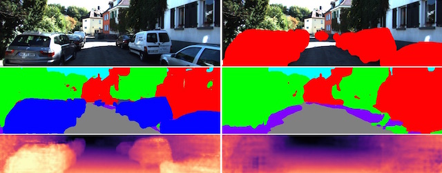
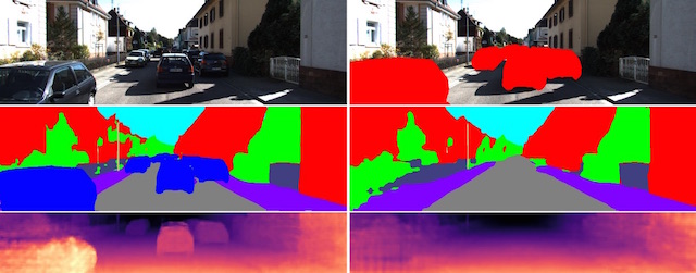
3 Additional qualitative results
The main paper already contains qualitative results of the final semantic BEV representation for the KITTI-Ros data set in Figure 8. Here, we provide additional examples for the KITTI-Anon and the Cityscapes data sets in Figures 3 and 4, respectively.
Moreover, we show a few additional examples of our representation including dynamic foreground objects like cars in Figure 5.
4 Semantic segmentation and depth prediction of visible pixels
The proposed semantic bird’s eye view representation assumes a semantic segmentation of the visible pixels as input in order to identify foreground objects which define occlusions of the scene. Any semantic segmentation module can be used and we picked a CNN architecture inspired by the PSP module [sam:Zhao17a]. Besides standard semantic segmentation, this CNN also predicts depth of all visible pixels with a second decoder similar in structure to [sam:Laina16a], which is required to estimate depth for 3D localization of dynamic foreground objects (or traffic participants) like cars and pedestrians.
For completeness, this section provides a quantitative evaluation of this CNN. Table 3 shows our results for semantic segmentation and depth prediction and Figure 6 provides some qualitative examples. For evaluating semantic segmentation we use mean IoU as in the main paper. For evaluating depth prediction, we present additional metrics that are typically used and defined in [sam:Eigen14a]: RMSE, RMSE-log, accuracy (with threshold of ), and absolute relative difference (ARD). Note that we use a down-scaled version of Cityscapes (by a factor of ) for this experiment because it significantly decreases runtime and memory consumption during training and evaluation.
| \topruleDataset | mIoU | RMSE | RMSE-log | ACC | ARD |
|---|---|---|---|---|---|
| \midruleKITTI-Anon | 69.63 | 4.129 | 0.158 | 89.56 | .0928 |
| KITTI-Ros [sam:Ros15a] | 59.02 | 3.976 | 0.172 | 86.73 | .1076 |
| Cityscapes [sam:Cordts16a] | 63.66 | 8.352 | 0.220 | 89.65 | .1113 |
| \bottomrule |