Sure Screening for Transelliptical Graphical Models
Abstract
We propose a sure screening approach for recovering the structure of a transelliptical graphical model in the high dimensional setting. We estimate the partial correlation graph by thresholding the elements of an estimator of the sample correlation matrix obtained using Kendall’s tau statistic. Under a simple assumption on the relationship between the correlation and partial correlation graphs, we show that with high probability, the estimated edge set contains the true edge set, and the size of the estimated edge set is controlled. We develop a threshold value that allows for control of the expected false positive rate. In simulation and on an equities data set, we show that transelliptical graphical sure screening performs quite competitively with more computationally demanding techniques for graph estimation.
some key words: High Dimensionality; Kendall’s tau; Partial Correlation; Sparsity; Undirected Graph
1 Introduction
Consider the random vector , and an undirected graph denoted by , where is the set of nodes, and is the set of edges describing the conditional dependence relationships among . A pair is contained in the edge set if and only if is conditionally dependent on , given all remaining variables .
In recent years, many methods have been developed to recover the structure of graphical models in the high dimensional setting. Many authors have studied the Gaussian graphical model, in which conditional dependence is encoded by the sparsity pattern of the inverse covariance matrix (Yuan and Lin,, 2007; Friedman et al.,, 2008; Rothman et al.,, 2008; Ravikumar et al.,, 2009, and references therein). Liu et al., (2009); Liu et al., 2012a introduced the nonparanormal distribution, which results from univariate monotonic transformations of the Gaussian distribution, and showed that the structural properties of the inverse covariance matrix of the Gaussian distribution carry over to the corresponding nonparanormal distribution. Ravikumar et al., (2010) and Anandkumar et al., (2012) considered recovering the structure of an Ising graphical model. Yang et al., (2012) studied a class of graphical models in which the node-wise conditional distributions arise from the exponential family. Moreover, Yang et al., (2014) and Chen et al., (2015) considered the problem of structure recovery for mixed graphical models.
Luo et al., (2015) proposed a computationally-efficient screening approach for Gaussian graphical models, which they called graphical sure screening (GRASS). They estimated an edge between the th and th nodes if the sample correlation between the th and th features exceeds some threshold . Then the th node’s estimated neighborhood contains the true neighborhood with very high probability, under certain simple assumptions. GRASS requires only operations, while most other existing methods for estimating the graph require computations (Friedman et al.,, 2008).
However, GRASS requires that the data follows a multivariate normal distribution. In many settings, a reliance on exact normality is not desirable (Liu et al.,, 2009; Liu et al., 2012a, ; Liu et al., 2012b, ). In this paper, we propose transelliptical GRASS, an extension of the GRASS procedure to the transelliptical graphical model family, introduced by Liu et al., 2012b . We show that under a certain set of simple assumptions, the desirable statistical properties held by GRASS are also held by transelliptical GRASS. However, due to the relaxation of multivariate normality, the graph that we estimate represents the partial correlation, rather than conditional dependence, among variables.
The rest of this paper is organized as follows. In Section 2, we provide some background on transelliptical graphical models, and present a useful property of Kendall’s tau statistic. In Section 3, we establish the theoretical properties for transelliptical sure screening, which include the sure screening property, size control of the selected edge set, and the control of the expected false positive rate. Furthermore, we provide a choice of the threshold value that leads to the aforementioned desirable properties. Simulation studies are presented in Section 4, and an application to an equities data set is shown in Section 5. We close with a discussion in Section 6.
2 Preliminaries
The transelliptical distribution (Liu et al., 2012b, ) is a generalization of the nonparanormal distribution (Liu et al.,, 2009; Liu et al., 2012a, ). The transelliptical distribution extends the elliptical distribution in much the same way that the nonparanormal extends the normal distribution. We first provide the definition of the elliptical distribution.
Definition 1.
Let and with . A -dimensional random vector has an elliptical distribution, denoted by , if it has a stochastic representation
| (2.1) |
where is a random vector uniformly distributed on the unit sphere in , is a scalar random variable independent of , and satisfies .
In Definition 1, indicates that and have the same distribution. Many multivariate distributions, such as the multivariate normal and the multivariate t-distribution, belong to the elliptical distribution family.
From now on, we assume that in (2.1) is a full rank matrix so that is positive definite. In addition, assume that has unit diagonal elements. We let denote the th entry of . We also assume that the scalar random variable in (2.1) has density and .
Definition 2.
A continuous random vector follows a -dimensional transelliptical distribution, denoted by , if there exist monotone univariate functions and a nonnegative random variable satisfying , such that . We refer to as the latent variables of .
Remark 1.
A random vector follows a nonparanormal distribution (Liu et al.,, 2009; Liu et al., 2012a, ) if there exist monotone univariate functions such that . Therefore, the transelliptical distribution is a strict extension of the nonparanormal distribution.
Given a transelliptical distribution , we can define an undirected graph , where , and if and only if — that is, if and only if the latent variables and are partially correlated (Liu et al., 2012b, ). In the special case of a nonparanormal distribution, a zero entry of the precision matrix further implies conditional independence between the corresponding pair of random variables.
Next, we present the definition and some theoretical properties of the Kendall’s tau statistic.
Definition 3.
Given independent draws from , such that is the value of the th variable in the th observation, the population-level Kendall’s tau statistic between and is defined as
| (2.2) |
The sample estimator of Kendall’s tau is defined as
| (2.3) |
Now suppose that we have independent draws from , such that is the value of the th variable in the th observation. Then there is a simple connection between the population-level Kendall’s tau statistic and .
Lemma 1.
(Liu et al., 2012b, ) For , we have .
Lemma 1 motivated Liu et al., 2012b to estimate using
| (2.4) |
3 Transelliptical Graphical Sure Screening
3.1 Proposed Approach
Suppose that we have independent draws from . We define to be the true edge set, and to be the true neighborhood for the th node. We propose to estimate and as follows,
| (3.1) |
and
| (3.2) |
where is some threshold value that we will specify in the following sections, and is defined in (2.4). We refer to and as the transelliptical graphical sure screening (transelliptical GRASS) estimators.
3.2 Theoretical Properties
We now present some theoretical properties of transelliptical GRASS. Proofs are in the Appendix.
Assumption 1.
For some constant and ,
Assumption 1 requires that the elements in the edge set correspond to sufficiently large values in the correlation matrix. We next present the sure screening property in Theorem 1.
Theorem 1.
Suppose that Assumption 1 holds, and that for some constants and . Let . Then there exist constants and such that
and
Conversely, if , then there exist constants and such that
| (3.3) |
Theorem 1 guarantees that the candidate edge set obtained from transelliptical GRASS contains the true edge set with high probability, which means the screening method will not result in false negatives with high probability. Moreover, (3.3) suggests that Assumption 1 is necessary up to a constant. The following corollary shows that under Assumption 1, transelliptical GRASS can recover the connected components of with high probability.
Corollary 1.
Suppose there are connected components in the graph , and that the th connected component contains the variables , where . That is, and are partially uncorrelated for . Suppose Assumption 1 and the conditions in Theorem 1 hold. Let . Then the connected components of are the same as the connected components of with probability at least .
Our next theorem will provide a bound on the size of . This requires an additional assumption.
Assumption 2.
There exist constants and such that , where is the largest eigenvalue of .
Assumption 2 allows the largest eigenvalue of the population covariance matrix to diverge as grows.
Theorem 2.
Next we propose a choice of the threshold that enables us to control the expected false positive rate, defined as , at a pre-specified value. Here, , and is defined in (3.1). This requires an additional assumption.
Assumption 3.
For the same as in Theorem 1,
Theorem 3.
3.3 A Second Look at Assumptions 1 and 3
Assumptions 1 and 3 involve placing conditions on the elements of corresponding to non-zero and zero elements of , respectively. These conditions are somewhat hard to interpret, since in general there is no simple relationship between the th elements of a matrix and its inverse . We now present a result from Luo et al., (2015) that allows us to re-formulate these assumptions as conditions on the elements of . We let and . Here, and indicate the largest and smallest eigenvalues of a matrix, respectively.
Proposition 1.
4 Simulation Studies
The simulation studies in this section are largely based on those in Luo et al., (2015).
4.1 Data Generation
Let be the number of features, and the number of observations. Motivated by the simulation study of Luo et al., (2015), we considered four ways of generating the edge set .
-
Simulation A:
For all , we set with probability . We then generated a matrix , where
(4.1) Finally, we created a positive definite matrix ,
(4.2) where is the smallest eigenvalue of , and denotes the identity matrix.
- Simulation B:
-
Simulation C:
For all , we set .
-
Simulation D:
We partitioned the features into equally-sized and non-overlapping sets, for . Then for all , we set . All other elements of were set to zero.
was rescaled to have diagonal elements equal to 1. We then generated observations from a distribution, and observations from a multivariate -distribution with degrees of freedom, mean zero, and correlation . After that, we applied four monotonic functions, , , , , to these observations with equal probability; this process gave us nonparanormal-distributed observations and transelliptical -distributed observations.
4.2 Control of False Positive Rate
Theorem 3 states that under certain conditions, performing transelliptical GRASS with , where is of the form (3.4), leads to control of the asymptotic expected false positive rate (FPR) at level . In Tables 1 and 2, we explore the control of the FPR in finite samples, for nonparanormal and transelliptical -distributed data. The FPR (defined as FP/(FP+TN)) and false negative rate (FNR; defined as FN/(TP+FN)) are reported for various values of the level of desired FPR control, . The size of the estimated edge set is also reported. Here and , and results are averaged over 250 simulated data sets.
Assumption 3 is the key for controlling the asymptotic expected false positive rate. In Simulation B, both and are block diagonal with ten completely dense blocks. So Assumption 3 holds in Simulation B. In Simulation D, all of the zero elements in the precision matrix also correspond to zero elements in , so that Assumption 3 holds exactly. As expected, the FPR is controlled successfully in Simulations B and D.
In contrast, in Simulations A and C, not all of the zero elements in the precision matrix correspond to zero elements in the correlation matrix . But Table 1 and Table 2 reveal that the FPR is still controlled well in these settings. This is because Assumption 3 only requires the elements in to correspond to small, though not necessarily zero, elements of . This assumption holds for most of the elements in and for Simulations A and C. Therefore, the FPR is also well-controlled in Simulations A and C.
Simulation A Simulation B Simulation C Simulation D FPR FNR FPR FNR FPR FNR FPR FNR 1e-04 542.46 3e-04 0.925 1611.6 2e-04 0.969 290.22 2e-04 0.819 920.38 2e-04 0.819 0.001 1579.76 0.0019 0.868 3472.04 0.0014 0.943 1071.96 0.0014 0.648 1580.36 0.0014 0.806 0.01 7426.36 0.013 0.762 10950.86 0.011 0.879 6125.34 0.011 0.382 6364.42 0.011 0.793 0.1 53548.1 0.104 0.551 59265.12 0.098 0.695 49926.3 0.098 0.111 49884.46 0.098 0.722 0.2 102830.74 0.202 0.446 108698.82 0.195 0.580 98455.7 0.196 0.055 98333.9 0.195 0.644 0.3 152029.24 0.301 0.368 157545.2 0.294 0.488 147546.26 0.294 0.031 147393.94 0.294 0.566 0.5 250794.72 0.500 0.244 254988.28 0.493 0.332 246989.82 0.493 0.012 246737.66 0.493 0.405
Simulation A Simulation B Simulation C Simulation D FPR FNR FPR FNR FPR FNR FPR FNR 1e-04 448.836 3e-04 0.941 1325.172 2e-04 0.975 240.52 2e-04 0.87 859.488 2e-04 0.833 0.001 1447.58 0.0018 0.889 3039.336 0.0015 0.952 1012.12 0.0015 0.721 1564.668 0.0015 0.813 0.01 7261.952 0.013 0.788 10340.736 0.011 0.892 6123.648 0.0112 0.466 6438.42 0.0111 0.794 0.1 53507.624 0.104 0.575 58758.12 0.099 0.713 50330.904 0.099 0.158 50297.052 0.099 0.721 0.2 102902.456 0.203 0.468 108367.908 0.197 0.598 99069.432 0.197 0.085 98909.556 0.197 0.642 0.3 152190.388 0.302 0.387 157358.224 0.295 0.504 148208.564 0.295 0.053 148021.74 0.295 0.563 0.5 250987.548 0.50 0.258 254984.984 0.494 0.344 247579.316 0.495 0.023 247400.096 0.494 0.404
4.3 Comparison to Existing Approaches
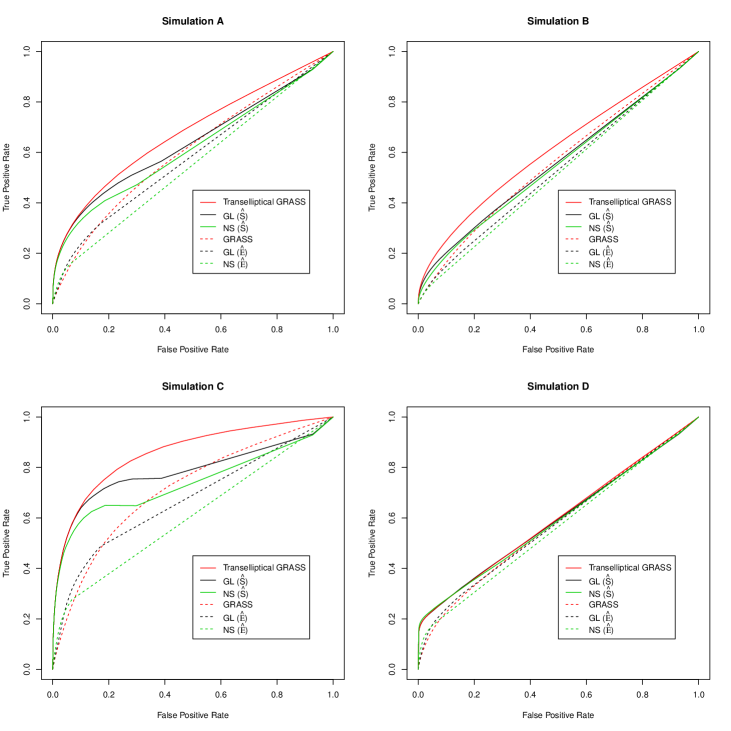
We first compare the performances of the graphical lasso (Friedman et al.,, 2008), neighborhood selection (Meinshausen and Bühlmann,, 2006), and transelliptical GRASS on nonparanormal data generated from Simulations A–D, with and . Let denote the simulated data matrix. We let GL() and NS() denote the results of the graphical lasso and the neighborhood selection applied to the estimated correlation matrix ; and we let GL() and NS() denote the results of the graphical lasso and neighborhood selection applied to , the Kendall’s tau estimator, defined in (2.4). Results are shown in Figure 1.
Transelliptical GRASS outperforms GL() and NS() in Simulation B. The sparsity patterns of and are identical, so the assumptions underlying transelliptical GRASS hold.
In Simulations A and C, most of the edges in correspond to large elements of , and most of the non-edges in correspond to small elements of . Consequently, transelliptical GRASS outperforms GL() and NS().
Simulation D was designed to violate Assumption 1; most of the elements in the edge set correspond to zero values in the correlation matrix . Therefore transelliptical GRASS does not perform well in Simulation D. But even in this undesirable setting, Figure 1 indicates that GL() and NS() do not perform much better than the transelliptical GRASS.
Not surprisingly, the original GRASS proposal (which involves thresholding ), GL(), and NS() perform poorly, because they are designed for Gaussian data rather than nonparanormal data.
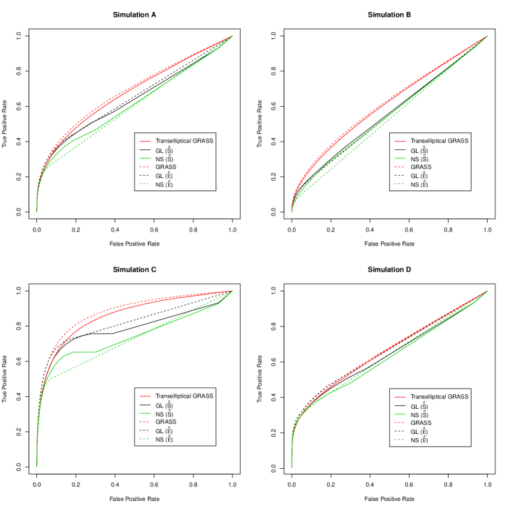
Finally, we compare the performance of the aforementioned methods on Gaussian data generated from Simulations A–D, with and . Figure 2 shows that the original GRASS proposal performs only slightly better than transelliptical GRASS on Gaussian data. This suggests that when the underlying distribution of the data is unknown, there is little cost (and potentially a large gain) associated with performing transelliptical GRASS instead of GRASS.
Overall, Figures 1 and 2 suggest that in these four settings, transelliptical GRASS performs competitively compared to some popular but computationally-intensive procedures for estimating a precision matrix.
5 Application to Equities data
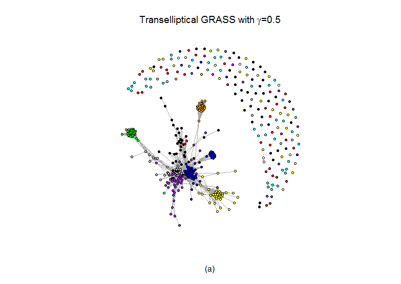
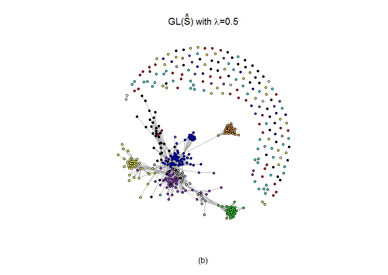
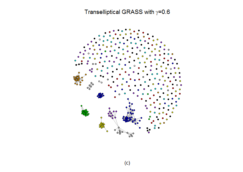
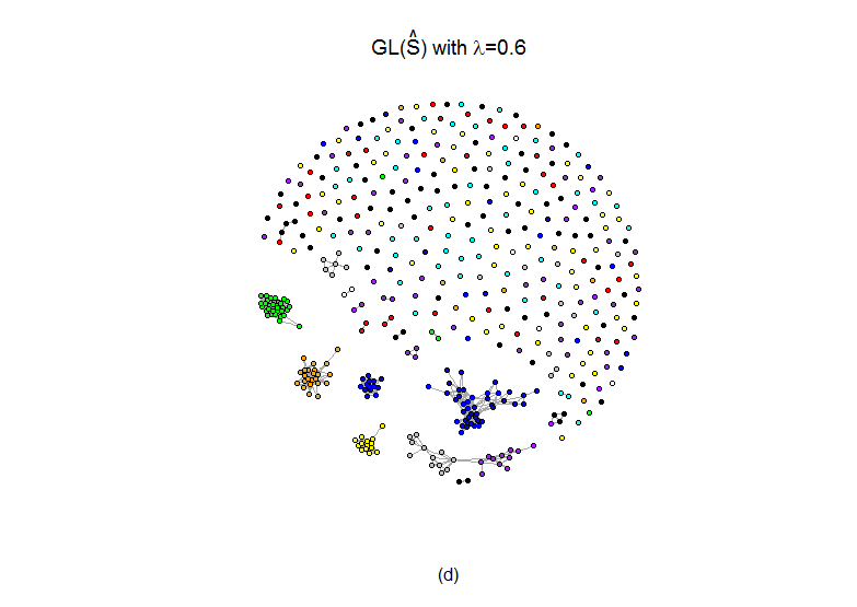
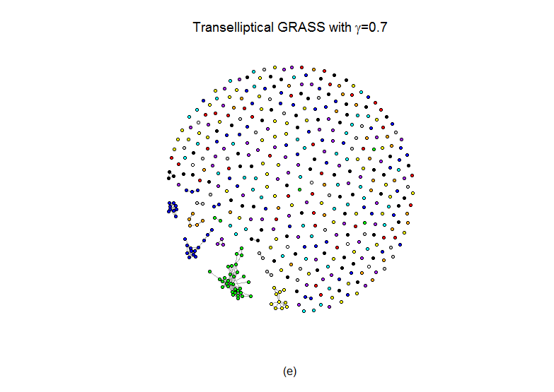
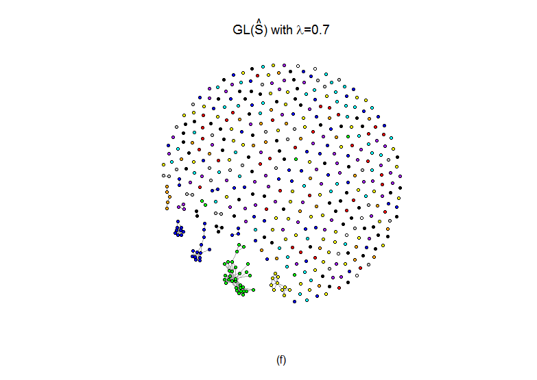
We examined the Yahoo! Finance stock price data, which is described in Liu et al., 2012b , and available in the huge package in R on CRAN. The data consists of 1258 daily closing prices for 452 stocks in the SP 500 index between January 1, 2003 and January 1, 2008. The stocks are categorized into 10 Global Industry Classification Standard (GICS) sectors.
Let denote the closing price of the th stock on the th day. We construct
a data matrix such that for and . We standardize each stock to have mean zero and standard deviation one, as in Tan et al., (2015).
We applied transelliptical GRASS with =0.5, 0.6, 0.7, and GL() with =0.5, 0.6, 0.7. Figure 3 indicates that in all estimated graphs, stocks from the same GICS sector tend to be highly-connected, indicating that both methods provide informative graph estimates. Furthermore, plots , , and of Figure 3 also show that the graph estimates from transelliptical grass and GL() are quite similar provided that . In fact, the arguments in Witten et al., (2011) can be used to establish the fact that when , the connected components of GRASS and GL() are identical.
6 Discussion
In this paper, we have proposed transelliptical GRASS, a simple and efficient procedure for recovering the structure of a high-dimensional transelliptical graphical model. Transelliptical GRASS is a natural extension of the GRASS proposal of Luo et al., (2015) to the non-normal setting. Transelliptical GRASS shares the attractive theoretical and computational properties of the original GRASS proposal. We have established that it performs almost as well as methods that assume Gaussianity when the data are Gaussian, and much better than methods that assume Gaussianity in the case of non-Gaussian data. Therefore, in general, there is little cost to applying transelliptical GRASS instead of the original GRASS proposal.
Appendix A Appendix
A.1 Proof of Theorem 1
Definition 4.
(Hoeffding, (1963), page 25) Let be independent random variables. For , a one-sample U-statistic takes the form
| (A.1) |
where , and the sum is taken over all -tuples of distinct positive integers not exceeding .
Lemma 2.
Recall from (2.3) that
Let , . Then the sample estimator is of the form (A.1) with and . Therefore, we can apply Lemma 2 with and , which yields
Next, we notice that
| (A.2) | |||||
The first equality results from directly applying Lemma 1 and our definition of . The first inequality results from applying the mean value theorem. It follows that
Here, the second inequality follows from Assumption 1, and the third inequality from the fact that along with (A.2).
Therefore, we have shown that
A similar argument can be used to establish that
Conversely, if , then there exists such that . This together with (A.2) implies that
so that the result holds.
A.2 Proof of Corollary 1
Proof.
It suffices to show that transelliptical GRASS will not result in edges between and for all with high probability.
This is the case when the event holds for all . As was shown in the proof of Theorem 1, . ∎
A.3 Proof of Theorem 2
Let
and
By definition, . On the set , if belongs to , it has to belong to . Thus, we conclude that . An argument similar to that in the proof of Theorem 1 can be used to show that
This implies that
| (A.3) |
Define . Then, by the definition of , it follows that
| (A.4) |
Furthermore,
| (A.5) |
where is the unit vector with a one in the th element and zeros elsewhere, and where the last equality results from the fact that the diagonal elements of are equal to .
A.4 Proof of Theorem 3
First, we verify the sure screening property (Section A.4.1). We then establish the control of the asymptotic expected false positive rate (Section A.4.2).
A.4.1 Verification of Sure Screening Property
A.4.2 Control of the Asymptotic Expected False Positive Rate
Next, we show that the choice of given in the statement of Theorem 3 leads to control of the asymptotic expected false positive rate at . The following lemma is used here.
Lemma 3.
Lemma 3 follows from Theorem 6 in Arvesen, (1969) in conjunction with Slutsky’s Theorem. It follows from an application of the delta method that
| (A.11) |
Therefore, for any , we have
where the convergence results from combining (A.11), Assumption 3, and the fact that the order of is much larger than that of because is of the same order as while by Assumption 3.
Consequently, the expected is controlled as desired,
where the last inequality results from the fact that .
References
- Anandkumar et al., (2012) Anandkumar, A., Tan, V. Y. F., Huang, F., and Willsky, A. S. (2012). High-dimensional Structure Estimation in Ising Models: Local Separation Criterion. The Annals of Statistics, 40:1346–1375.
- Arvesen, (1969) Arvesen, J. N. (1969). Jackknifing U-Statistics. The Annals of Mathematical Statistics, 40:2076–2100.
- Callaert and Veraverbeke, (1981) Callaert, H. and Veraverbeke, N. (1981). The Order of the Normal Approximation for a Studentized U-Statistic. The Annals of Statistics, 9:194–200.
- Chen et al., (2015) Chen, S., Witten, D., and Shojaie, A. (2015). Selection and estimation for mixed graphical models. Biometrika, 102(1):47–64.
- Fligner and Rust, (1983) Fligner, M. A. and Rust, S. W. (1983). On the independence problem and Kendall’s tau. Communications in Statistics - Theory and Methods, 12:1597–1607.
- Friedman et al., (2008) Friedman, J., Hastie, T. J., and Tibshirani, R. J. (2008). Sparse inverse covariance estimation with the graphical lasso. Biostatistics, 9:432–441.
- Hoeffding, (1963) Hoeffding, W. (1963). Probability inequalities for sums of bounded random variables. Journal of the American Statistical Association, 58:13–30.
- Lee, (1985) Lee, A. J. (1985). On estimating the variance of a U-statistic. Communications in Statistics - Theory and Methods, 14:289–302.
- (9) Liu, H., Han, F., Yuan, M., Lafferty, J., and Wasserman, L. (2012a). High-dimensional semiparametric Gaussian copula graphical models. The Annals of Statistics, 40:2293–2326.
- (10) Liu, H., Han, F., and Zhang, C. (2012b). Transelliptical graphical models. In Advances in Neural Information Processing Systems 25, pages 809–817.
- Liu et al., (2009) Liu, H., Lafferty, J., and Wasserman, L. (2009). The nonparanormal: Semiparametric estimation of high dimensional undirected graphs. Journal of Machine Learning Research, 10:2295–2328.
- Luo et al., (2015) Luo, S., Shi, C., Song, R., Xie, Y., and Witten, D. (2015). Sure Screening for Gaussian Graphical Models. to appear.
- Meinshausen and Bühlmann, (2006) Meinshausen, N. and Bühlmann, P. (2006). High-dimensional graphs and variable selection with the lasso. The Annals of Statistics, 34:1436–1462.
- Ravikumar et al., (2009) Ravikumar, P., Lafferty, J., Liu, H., and Wasserman, L. (2009). Sparse additive models. Journal of the Royal Statistical Society: Series B (Statistical Methodology), 71:1009–1030.
- Ravikumar et al., (2010) Ravikumar, P., Wainwright, M. J., and Lafferty, J. D. (2010). High-dimensional Ising Model Selection Using L1-Regularized Logistic Regression. The Annals of Statistics, 38:1287–1319.
- Rothman et al., (2008) Rothman, A. J., Bickel, P. J., Levina, E., and Zhu, J. (2008). Sparse permutation invariant covariance estimation. Electronic Journal of Statistics, 2:494–515.
- Sen, (1977) Sen, P. K. (1977). Some Invariance Principles Relating to Jackknifing and Their Role in Sequential Analysis. The Annals of Statistics, 5:316–329.
- Tan et al., (2015) Tan, K. M., Witten, D., and Shojaie, A. (2015). The cluster graphical lasso for improved estimation of Gaussian graphical models. Computational Statistics and Data Analysis, 85:23–36.
- Witten et al., (2011) Witten, D. M., Friedman, J. H., and Simon, N. (2011). New insights and faster computations for the graphical lasso. Journal of Computational and Graphical Statistics, 20(4):892–900.
- Yang et al., (2012) Yang, E., Allen, G., Liu, Z., and Ravikumar, P. (2012). Graphical models via generalized linear models. In Advances in Neural Information Processing Systems 25, pages 1367–1375.
- Yang et al., (2014) Yang, E., Ravikumar, P., Allen, G., Baker, Y., Wan, Y., and Liu, Z. (2014). A General Framework for Mixed Graphical Models. arXiv:1411.0288.
- Yuan and Lin, (2007) Yuan, M. and Lin, Y. (2007). Model selection and estimation in the Gaussian graphical model. Biometrika, 94:19–35.