.
Surface Solitons in Three Dimensions
Abstract
We study localized modes on the surface of a three-dimensional dynamical lattice. The stability of these structures on the surface is investigated and compared to that in the bulk of the lattice. Typically, the surface makes the stability region larger, an extreme example of that being the three-site “horseshoe”-shaped structure, which is always unstable in the bulk, while at the surface it is stable near the anti-continuum limit. We also examine effects of the surface on lattice vortices. For the vortex placed parallel to the surface this increased stability region feature is also observed, while the vortex cannot exist in a state normal to the surface. More sophisticated localized dynamical structures, such as five-site horseshoes and pyramids, are also considered.
I Introduction
Surface waves have been a subject of interest in a variety of contexts, including surface plasmons in conductors Barnes and optical solitons in waveguide arrays Christo in physics, surface waves in isotropic magnetic gels Bohlius in chemistry, water waves in the ocean in geophysical hydrodynamics, and so on. Quite often, features exhibited by such wave modes have no analog in the corresponding bulk media, which makes their study especially relevant. In particular, a great deal of interest has been drawn to nonlinear surface waves in optics. It was shown theoretically Makris and observed experimentally Suntsov that discrete localized nonlinear waves can be supported at the edge of a semi-infinite array of nonlinear optical waveguide arrays. Such solitary waves were predicted to exist not only in self-focusing media (as in the above-mentioned works), but also between uniform and self-defocusing media Makris ; kartprl , or between self-focusing and self-defocusing media (e.g. in debra ). They have been subsequently observed in media with quadratic Sivilogou and photorefractive rosberg ; smirnov nonlinearities. In the two-dimensional (2D) geometry, stable topological solitons have been predicted in a saturable medium Kartashov , which constitute generalizations to lattice vortex solitons predicted in Ref. Malomed . Quasi-discrete vortex solitons have been experimentally observed in a self-focusing bulk photorefractive medium Neshev . Theoretical predictions for a variety of species of discrete 2D surface solitons Susanto ; Makris2 ; Kartashov2 ; BluKon ; Vicencio , corner modes Makris2 ; BluKon , as well as surface breathers BluKon , were reported. Subsequent work has resulted in the experimental observation of 2D surface solitons, both fundamental ones and multi-pulse states, in photorefractive media christo2d , as well as in asymmetric waveguide arrays written in fused silica kart2d . Recently, surface solitons in more complex settings, such as chirped optical lattices in 1D and 2D kart_mol1 ; kart_mol2 , at interfaces between photonic crystals and metamaterials shadrivov , and in the case of nonlocal nonlinearity moti1 ; moti2 , have emerged.
Nearly all these efforts have been aimed at the study of surface solitons in 1D and 2D geometries. The only 3D setting examined thus far assumed a truncated bundle of fiber-like waveguides, incorporating the temporal dynamics in longitudinal direction to produce 3D “surface light bullets” in Ref. dumitru (the respective 2D surface structures were examined in Ref. dumitru1 ).
Our aim in the present work is to extend the analysis to surface solitons in genuine 3D lattices. Our setup is relevant to a variety of applications including, e.g., crystals built of microresonators trapping photons earlier1 , polaritons earlier2 , or Bose-Einstein condensates in the vicinity of an edge of a strong 3D optical lattice morsch ; bloch . In particular, we report results for discrete solitons at the surface of a 3D lattice, i.e., 3D localized states that are similar to relevant objects studied in the 2D setting of Ref. Susanto . Thus, we will study localized states such as dipoles and “horseshoes” abutting on a set of three lattice sites, but also states that are specific to the 3D lattice. A variety of species of such solitons is examined below, and their stability on the surface is compared to that in the bulk. Some localized structures, such as dipoles, may be placed either normal or parallel to the surface. We demonstrate that, typically, the enhanced contact with the surface increases the stability region of the structure. Physically, this conclusion may be understood by the fact that the surface reduces the local interactions to fewer neighbors, rendering the system “more discrete”, hence more stable (by pushing the medium further away from the continuum limit, where all solitons would be unstable against the collapse). This effect is remarkable, e.g., for the three-site horseshoes which are never stable in the bulk, but get stabilized in the presence of the surface. However, the surface may also have an adverse effect, inhibiting the existence of a particular mode. The latter trend is exemplified by discrete vortices, which, if placed parallel to the surface, feature enhanced stability as compared to the bulk-mode counterpart, but cannot exist with the orientation perpendicular to the surface. Surface-induced effects of a different kind, which are less specific to discrete systems, are induced by the interaction of a particular localized mode with its fictitious “mirror image”. In terms of lattice models, the approach based on the analysis of the interaction of a real mode with its image was proposed in Ref. Christodoulides .
To formulate the model, we introduce unit vectors , , and and define lattice sites by with integer . We assume that the lattice occupies a semi-infinite space, , and its dynamics obeys the discrete nonlinear Schrödinger (DNLS) equation in its usual form,
| (1) |
Here is a complex discrete field, is the coupling constant, stands for the time derivative, the parameter determines the sign of the nonlinearity (focusing or defocusing respectively), and is the 3D discrete Laplacian:
| (2) |
for , while for the term with subscript index is to be dropped (note that is the direction normal to the surface).
It is interesting to point out here that an approach towards understanding the dynamics of Eq. (1) in the vicinity of the surface can be based on the above-mentioned concept of the fictitious mirror image, formally extends the range of up to , supplementing the equation with the anti-symmetry condition,
| (3) |
Indeed, this condition implies , which is equivalent to the summation restriction in Eq. (2) as defined above.
To confine the analysis to localized solitary wave modes, we impose zero boundary conditions, at and . Additionally, in Eq. (2) —this parameter is introduced for convenience (see Sec. III.2) and can be freely rescaled using the transformation for an appropriate choice of and time rescaling. Stationary solutions to Eq. (1) will be sought for as , where is the frequency and the lattice field obeys the equation
| (4) |
Our presentation is structured as follows. The following section recapitulates the necessary background for the prediction of the existence and stability of lattice solitons. In section III, we report a bifurcation analysis for various surface states, treated as functions of coupling constant , with emphasis on the comparison with bulk counterparts of these states. Section IV reports the study of the evolution of unstable surface states. Finally, section V summarizes our findings and presents our conclusions.
II The theoretical background
First, we outline some general properties of the model. Equation (1) conserves two dynamical invariants, namely the norm ,
| (5) |
and the Hamiltonian ,
| (6) |
where the asterisk stands for complex conjugation. Stationary solutions to Eq. (4) with are connected by the staggering transformation ABK ; BluKon : if is a solution for some and , then is a solution for and . Consequently, it is sufficient to perform the analysis of stationary solutions, including their stability, for a single sign of the nonlinearity; thus, below we will fix (corresponding to the case of onsite self-attraction).
Solutions to Eq. (4) in half-space , subject to boundary condition for , as defined above, may be continued anti-symmetrically for the entire 3D space by setting for and for . Then, according to results of Ref. Weinstein , this leads to an immediate conclusion, namely that there exists a minimum norm necessary for the existence of localized surface states in the present model. In other words, no surface modes survive in the limit of . In this connection, it is relevant to note that numerical findings that will be presented below were obtained, of course, for finite cubic lattices where, strictly speaking, there is no lower limit for necessary for the existence of localized modes BluKon . At this point, we have to specify that speaking about localized modes in a finite lattice we understand solutions which are localized on a number of cites much smaller than the total number of sites in the chosen direction used for numerical simulations. Next we recall that generally speaking, there exist several branches of the nonlinear localized modes, i.e. for a given one can find localized excitations at different values of the norm . Using the natural terminology we refer to higher/lower branches speaking about solutions with larger/smaller norm. In this classification the surface modes we are dealing with correspond to higher branches of the solutions of the respective finite lattices, i.e., their norm cannot be made arbitrarily small (see also the relevant discussion below in Section III.2).
To find solution families, we start with the anti-continuum (AC) limit, Pelinovsky . In this limit, the lattice field is assumed to take nonzero values only at a few (“excited”) sites, which determines the profile of the configuration to be seeded. The continuation of the structure to is determined by the Lyapunov’s reduction theorem Golubitsky . More specifically, the solution is expanded as a power series in , the solvability condition at each order being that the respective projection to the kernel generated by the previous order does not give rise to secular terms Pelinovsky .
The linear stability is then studied, starting from the usual form of the perturbed solution,
| (7) |
where is a formal small parameter, and is a stability eigenvalue associated with eigenvector . Substituting this into Eq. (1) yields the linearized system,
which can be cast in the form
| (8) |
where and are vectors composed by elements and , respectively, while the matrices () are given by,
| (9) | |||||
An underlying stationary solution is (spectrally) unstable if there exists a solution to Eq. (8) with . Otherwise, the stationary solution is classified as a spectrally stable one. As explained in Ref. Pelinovsky1d , the Jacobian of the above mentioned solvability conditions is intimately connected to the full eigenvalue problem. More specifically, if the eigenvalues of the eigenvalue problem of the Jacobian (where is the number of excited sites at the AC limit), then the near-zero eigenvalues of the full stability problem can be predicted to be , where is the number of lattice sites that separate the adjacent excited nodes of the configuration at the AC limit.
III The bifurcation analysis
III.1 Existence and stability of surface structures
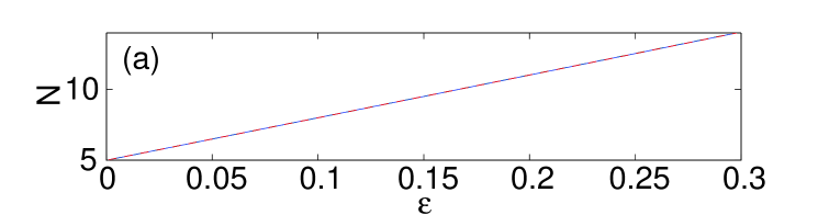
In this section we study, by means of numerical methods, the existence and stability of various 3D configurations and compare the results to the corresponding analytical predictions. These configurations are obtained by starting from the AC limit , and are continued to , using fixed-point iterations. For all the numerical results presented in this work, we fix the normalization [see Eq. (4)], and use a lattice of size , unless stated otherwise. Also, for the presentation of the numerical results, we replace the triplet by , i.e., the surface corresponds to .
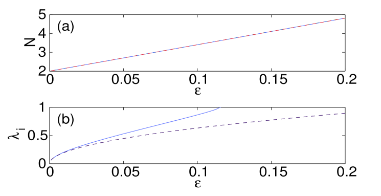
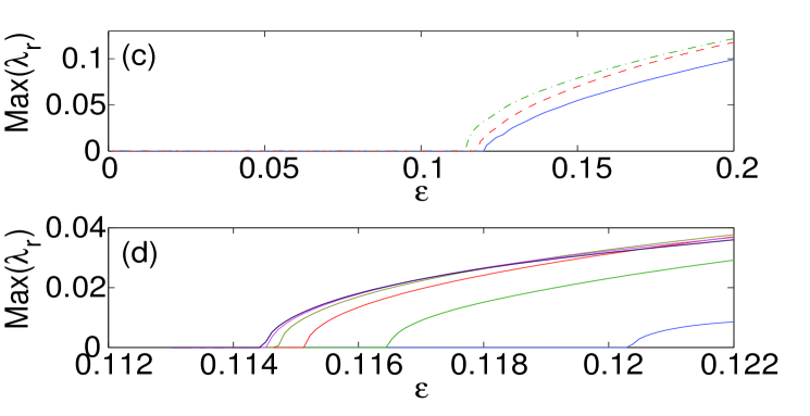
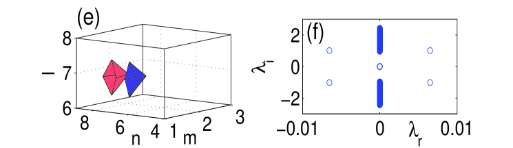
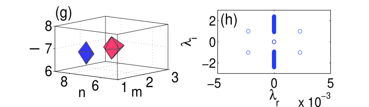
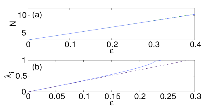
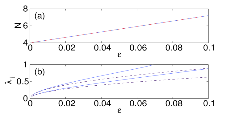
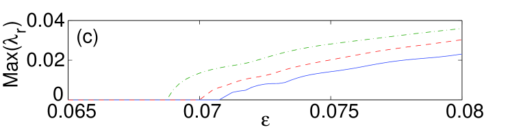
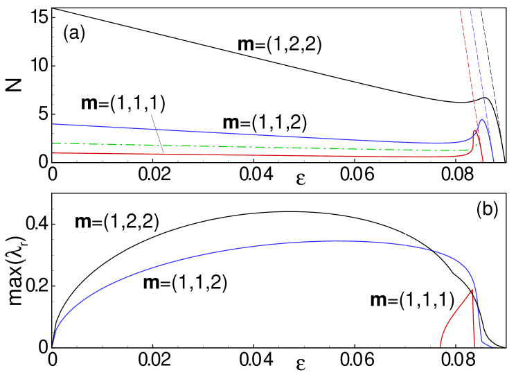
We start by examining dipoles aligned parallel or normal to the surface. Panel (a) in Fig. 1 shows the norm of such states versus coupling constant , while panel (b) depicts the imaginary part of the stability eigenvalues for the bulk dipole, produced by the theory outlined in the previous section [dashed (black) lines], and by the numerical computations [solid (blue) lines]. It is worth mentioning that, for all the different configurations that we report in this manuscript, we display the imaginary part of the stability eigenvalue only for the bulk mode since the difference between the curves for the different variants (bulk, parallel or normal to the surface) is minimal. It should be noted however that the contact with the surface may produce higher order (smaller) eigenvalues that are not present in its bulk counterpart (results not shown here). The theoretical prediction for the stability eigenvalues is , which, as expected, is the same as in an out-of-phase (twisted) 1D mode analyzed in Ref. Pelinovsky1d , since the structure is nearly one-dimensional, along the line connecting the two excited sites. Panel (c) in Fig. 1 compares the largest instability growth rate as a function of for the bulk dipoles [dash-dotted (green) line] and those oriented normally and parallel to the surface [dashed (red) and solid (blue) lines, respectively]. It is seen that the stability interval of the dipoles increases as its contact with the surface strengthens, in accordance with the arguments presented above. In the case of the bulk dipole, the instability occurs for values of the coupling constant in between and . From now on, when reporting computed instability thresholds, we will use the lower bound for (e.g., in the above example) with the understanding that we always used the same resolution in . For the dipole set normally to the surface, we observe the onset of instability at , while for the parallel-oriented one at . In panels (e)–(h) of Fig. 1 we also depict the shapes of the normal and parallel dipoles, just below the instability threshold, along with their corresponding spectral stability planes.
The stabilizing effects exerted by the surface depend, in a great measure, on the distance of the configuration from the surface, namely, the further away the configuration from the surface, the lesser the effect is. This property is clearly seen in panel (d) of Fig. 1, where we plot the (in)stability eigenvalue as a function of the coupling for several values of the separation of the parallel dipole from the surface. The curves, from right to left, depict the results for the dipole set at the distance of 0, 1, …, 5 sites away from the surface (0 sites refers to the dipole sitting on the surface). As the panel demonstrates, the stability interval is reduced as the dipole is pulled away from the surface, converging towards a bulk dipole.
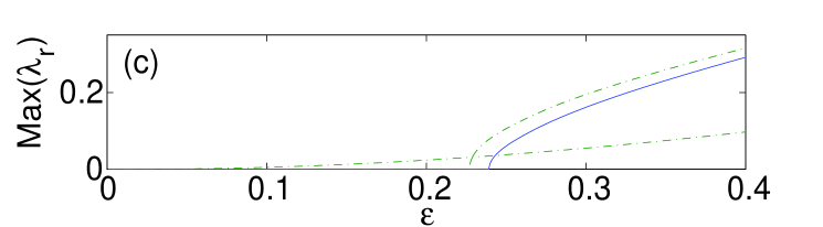
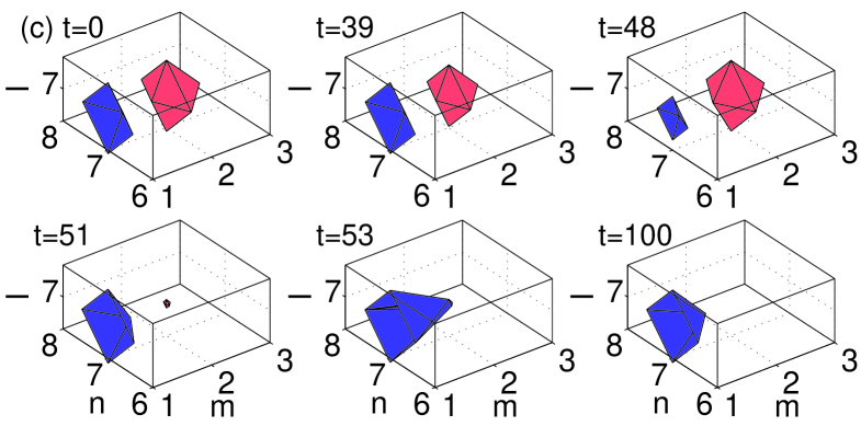
Let us now consider the “horseshoe” configurations, for which the presence of the surface is critical to their stability. In Fig. 2 we depict the properties of a three-site horseshoe, which actually is a truncated version of a quadrupole, cf. the 2D situation Susanto . As before, panel (a) in Fig. 2 shows the norm versus , while panels (b) and (c) compare the stability of the bulk horseshoe (the dash-dotted line) and ones built near the surface (the solid line). While the bulk horseshoes are always unstable, similar to their 2D counterparts Susanto , the ones placed near the surface are stable at small , destabilizing at . Panels (d)-(e) in Fig. 2 show the configuration for the coupling just below the instability threshold, along with the respective spectral plane. The analytical expressions for stable eigenvalues are , , , cf. the expressions obtained in Ref. Susanto for the 2D horseshoes.
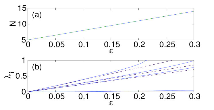
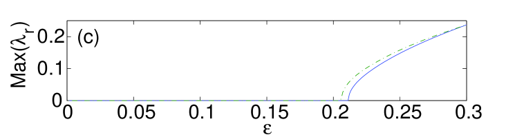
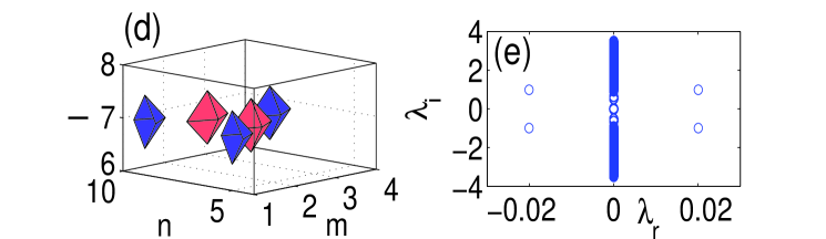
Figure 3 illustrates the same features as before but for the five-site horseshoe. Unlike its three-site cousin, the bulk five-site horseshoe is stable up to a critical value of the coupling, , while the surface variant has it stability region . The eigenvalues of the linearization in this case can be computed similar to those for the three-site modes Susanto , as outlined above (cf. also Ref. Pelinovsky ), which eventually yields , , , , and , in good agreement with the corresponding numerical results, as shown in panel (b) Fig. 3.
Next we consider the quadrupole configuration, see Fig. 4. The surface again exerts a stabilizing effect, albeit a weaker one, when the quadrupole is placed normally and parallel to the surface. In the bulk, the quadrupole loses stability at , while the normal and parallel surface quadrupoles have stability thresholds, respectively, at and . The analytical approximation for the stability eigenvalues in this case are (a double eigenvalue), , and a zero eigenvalue, which accurately capture the numerical findings depicted in panel (b) of Fig. 4.
In Fig. 5 we present the results for four-site vortices. This configuration, in contrast to the previous ones, is described by a complex solution. In the AC limit, the vortex occupies the same excited sites as the above-mentioned quadrupole, but the phase profile, , emulates that of the vortex of charge Malomed ; Pelinovsky . The bulk four-site vortex (which was discussed in Ref. earlier3 ) loses its stability at , while the vortex parallel to the surface features an extended stability region, up to . However, the surface in this case prohibits the existence of a vortex that would be oriented normally to the surface layer, similarly to what was found for 2D lattice vortices Susanto .
The simplest explanation for the complete absence of the solution normal to the surface, compared with that of an existing vortex waveform parallel to the surface can arguably be traced in the interaction of such vortices in the half-space with their fictitious image (if the domain is equivalently extended to the full space). In the case of the vortex parallel to the surface, the situation is tantamount to the vortex cube structures examined in vor3dnew ; Pelinovsky3d , for which it was established in Pelinovsky3d that the persistence conditions are satisfied (and, in fact, that such structures consisting of two out-of-phase vortices should be linearly stable close to the AC limit). On the other hand, for the case normal to the surface, by examining the relevant interactions it can be observed (at an appropriately high order) that the persistence conditions of Pelinovsky ; Pelinovsky1d ; Pelinovsky3d can not be satisfied and hence the structure can not be continued beyond the AC limit. That is why the structure can never be observed to exist irrespectively of the smallness of .
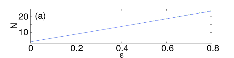
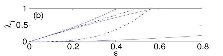
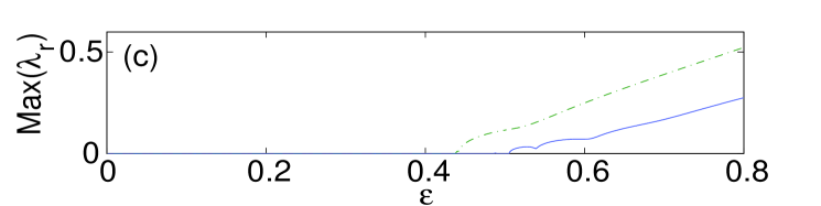
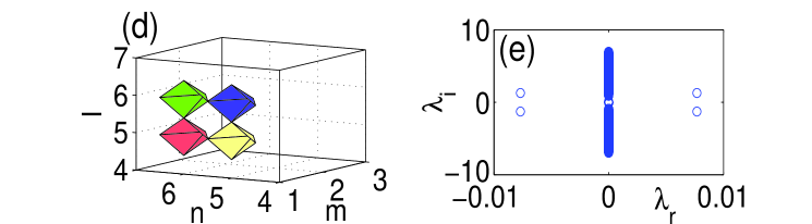
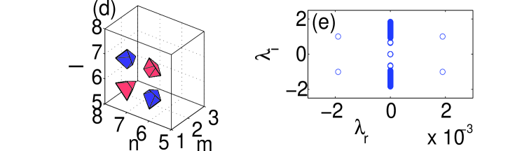
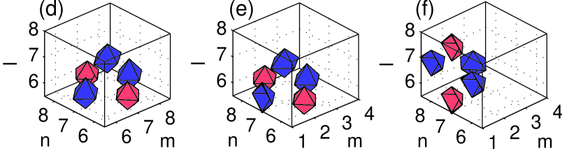
The next species of stationary lattice solutions is a pyramid-shaped structure, with characteristics displayed in Fig. 6, whose base is a rhombus composed of four sites. The remaining out-of-plane vertex site must have phase or , since the phase values and at this site do not produce a solution. The full set of pyramids (bulk, normal, parallel —see panels (d)–(f) of Fig. 6) is completely unstable, as seen in panel (c) of Fig. 6, the surface producing no stabilizing effect on it. This strong instability actually arises at the lowest order in the analytical eigenvalue calculations, which yield , , , , and , once again in very good agreement with the full numerical results of Fig. 6.
III.2 Small-amplitude modes in a finite lattice
Since our numerical investigation of the surface modes uses a finite lattice, which allow the existence of small-amplitude modes (ones with the zero threshold in terms of the norm — cf. discussion in Sec. II), here we briefly consider the modes in a finite lattice having the small-amplitude limit. Our aim is to show that these modes belong to lower branches, as compared with the “normal” surface modes considered above. To this end, we concentrate on the lattice of size lattice, subject to the zero boundary conditions, which imply that discrete Laplacian (2) is modified at surfaces and () by setting the fields at sites and , respectively, equal to zero. For the sake of definiteness, we fix here in Eq. (2).
To determine the norm of small-amplitude modes we follow Ref. BluKon , and look for a solution to Eq. (4) with the amplitude and coupling constant being represented as series
in powers of small parameter , which vanishes in the limit of the infinite lattice (); in other words, small characterizes the “largeness” of the lattice. We focus on real solutions here.
Substituting expansions (LABEL:eps) into Eq. (4) and gathering terms of the same order in , we rewrite Eq. (4) in the form of a set of equations:
| (11) |
Here , , hence Eq. (11) with gives rise to a linear eigenmode,
| (12) |
with the respective approximation for the lattice coupling constant,
| (13) |
parameterized by vector . At the same time, considering the solvability conditions for , which amounts to demanding the orthogonality of and , we obtain corrections to the coupling constants,
| (14) |
It follows from Eq. (14) that each of the linear modes (12) is uniquely extended into a small-amplitude nonlinear one. These modes are characterized by the linear dependence of the norm on coupling constant :
| (15) |
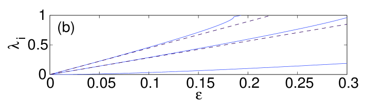
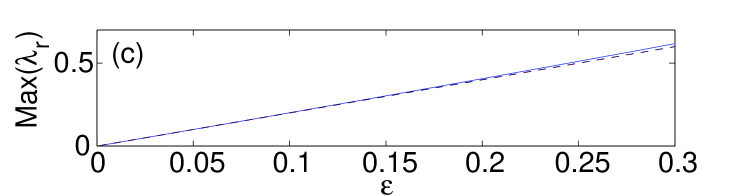
From Eq. (15) it follows that each mode, parameterized by vector , exists when belongs to the interval . The validity of approximation (15) is corroborated by the coincidence of analytical and numerical results in the vicinity of (as shown in Fig. 7), where these modes reaches their small-amplitude limit. Such a property of these modes differs considerably from the case of the surface modes which do not possess the small-amplitude limit and require some minimal value of the norm (for the normal dipole, depicted in Fig. 7 by dash-dotted line, the minimal norm is ). Panel (b) in Fig. 7 shows that only the mode, parameterized by vector , is stable for close to , while other modes are completely unstable.
IV Dynamics
In this section we examine the nonlinear evolution of the various configurations, displaying the results in a set of figures (see Figs. 8–12). In each case, the evolution is initiated at a value of the coupling taken beyond the instability threshold, and an initial small random perturbation is applied in order to expedite the onset of the instability.
 |
 |
 |
 |
 |
 |
 |
 |
 |
 |
 |
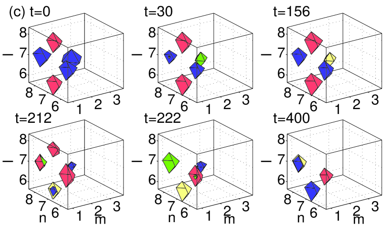 |
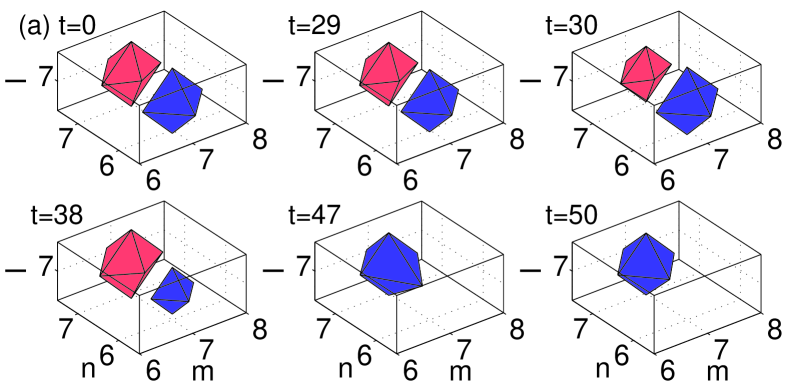
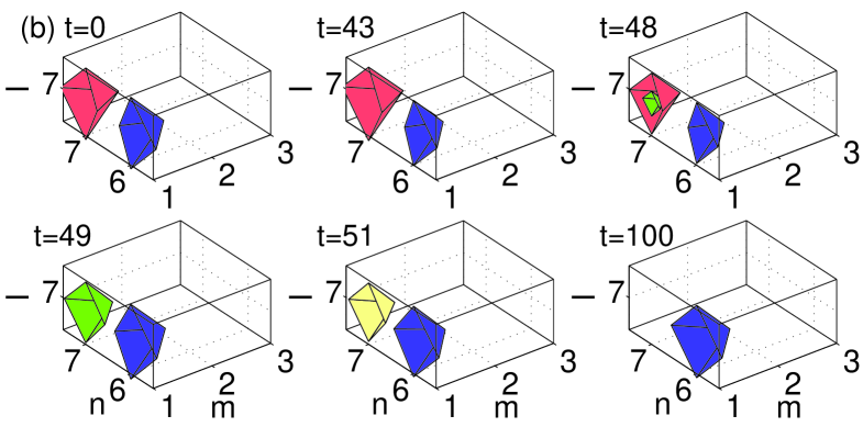
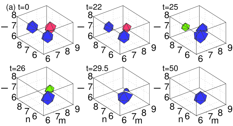
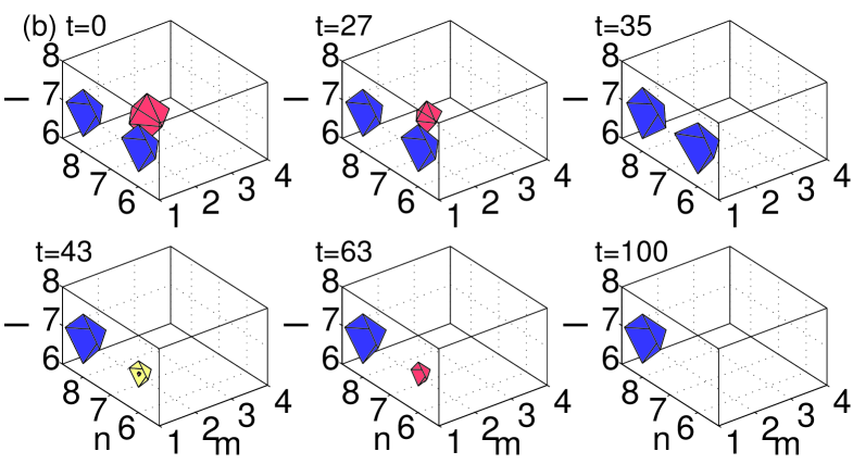
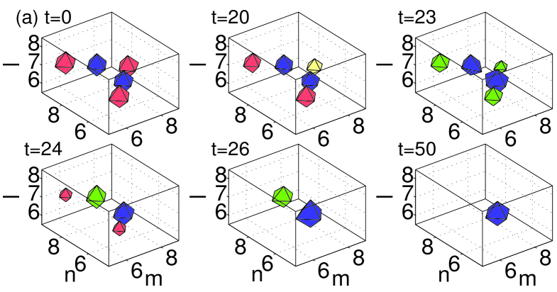
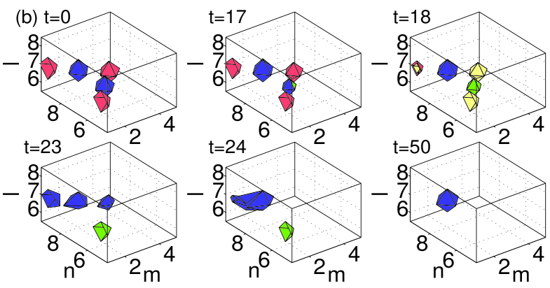
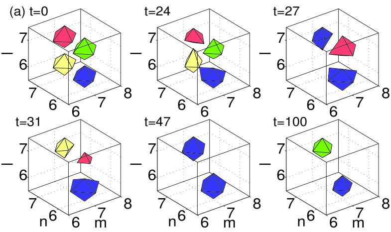
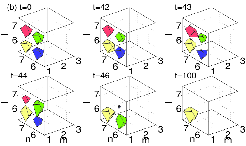
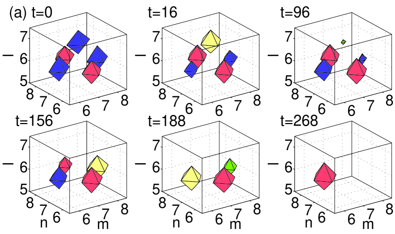
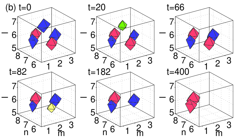
All the figures display the evolution of the instability at six different moments of time, starting at , and ending at a time well beyond the point at which the instability manifests itself. All configurations that were predicted above to be unstable through nonzero real parts of the (in)stability eigenvalue indeed exhibit instability dynamics, which eventually results in a transition to a different configuration. In the case of the dipoles and horseshoes, Figs. 8–10 show a spontaneous transition to monopole patterns, i.e., ones centered around a single excited site. On the other hand, in the case of the vortices and pyramids shown in Figs. 11–12, a few sites may remain essentially excited at the end of the evolution. The monopole is, obviously, the most robust dynamical state in the lattice system, with the widest stability interval, in comparison with other discrete structures. This simplest state becomes unstable, for given , only at values of the coupling constant earlier3 . Another structure with a relatively wide stability region is the dipole (the more stable the wider the distance between its constituent sites vor3dnew ), consonant with the observation that some of the structures (especially ones with a large number of excited sites, such as vortices and pyramids) dynamically transform into dipoles.
Generally speaking, the exact scenario of the nonlinear evolution and the finally established state depend on details of the initial perturbation. In the figures, each configuration is shown by iso-level contours of distinct hues. In particular, dark gray (blue) and gray (red) are iso-contours of the real part of the solutions, while the light gray (green) and very light gray (yellow) colors depict the imaginary part of the same solutions.
A case that needs further consideration is that of the three-site horseshoe. As observed from the stability analysis presented in Fig. 2, this horseshoe in the bulk gives rise to a small unstable purely real eigenvalue for all values of , see the lower green dashed-dotted curve in panel (c) of the figure. Despite the presence of this eigenvalue, the evolution of the unstable bulk three-site horseshoe is predominantly driven by the unstable complex eigenvalues, if any (in fact, for , see the dashed-dotted (green) line of Fig. 2.(c)). A careful analysis of the instability corresponding to the small purely real eigenvalue for (i.e., before the complex eigenvalues become unstable) reveals that the corresponding dynamics amounts to an extremely weak exchange of the norm between the two in-phase excited sites (see Fig. 2). The norm exchange is driven by the corresponding unstable eigenfunction, which looks like a dipole positioned at the two aforementioned in-phase sites. The difficulty in observing this evolution mode is explained by the fact that, in the course of the norm exchange, only of the total norm is actually transferred between the two sites. Furthermore, as mentioned earlier, the corresponding small real eigenvalue is completely suppressed by the surface (see panel (c) in Fig. 2). It is worth noting that such stable three-site horseshoe surface structures may also be generated by the evolution of more complex unstable waveforms, such as the five-site pyramids placed normally to the surface, see the bottom panel in Fig. 12.
V Conclusions
In this work, we have investigated localized modes in the vicinity of a two-dimensional surface, in the framework of the three-dimensional DNLS equation, which is a prototypical model of nonlinear dynamical lattices. We have found that the surface may readily stabilize localized structures that are unstable in the bulk (such as three-site horseshoes), and, on the other hand, it may inhibit the formation of some other structures that exist in the bulk (such as vortices which are oriented normally to the surface, although ones parallel to the surface do exist and have their stability region; a qualitative explanation to these features was proposed, based on the analysis of the interaction of the vortical state with its “mirror image”). The most typical surface-induced effect is the expansion of the stability intervals for various solutions that exist in the bulk and survive in the presence of the surface. This feature may be attributed to the decrease, near the surface, of the number of neighbors to which excited sites couple, since the approach to the continuum limit, i.e., the strengthening of the linear couplings to the nearest neighbors, is responsible for the onset of the instability or disappearance of all the localized stationary states in the three-dimensional dynamical lattice.
On the other hand, while the techniques elaborated in Refs. Pelinovsky1d ; Pelinovsky ; Pelinovsky3d for the analysis of localized states in bulk lattices are quite useful in understanding the dominant stability properties of the solutions, the surface gives rise to specific effects, such as the stabilization of higher-order solutions or the suppression of some types of vortex structures, which cannot be explained by these methods. Therefore, it would be very relevant to modify these techniques, which are based on the Lyapunov-Schmidt reductions, so as to take the presence of the surface into regard.
References
- (1) W. L. Barnes, A. Dereux, and T. W. Ebbesen, Nature 424, 824-830 (2003).
- (2) D. N. Christodoulides, F. Lederer, and Y. Silberberg, Nature 424, 817-823 (2003).
- (3) S. Bohlius, H. R. Brand and H. Pleiner, Z. Phys. Chem. 220, 97-104 (2006).
- (4) K. G. Makris, S. Suntsov and D. N. Christodoulides, G. I. Stegeman, Opt. Lett. 30, 2466 (2005); M. I. Molina, R. A. Vicencio, and Yu. S. Kivshar, Opt. Lett. 31, 1693 (2006).
- (5) S. Suntsov, K. G. Makris, D. N. Christodoulides, G. I. Stegeman, A. Hache, R. Morandotti, H. Yang, G. Salamo, and M. Sorel, Phys. Rev. Lett. 96, 063901 (2006).
- (6) Y. V. Kartashov, V. A. Vysloukh, and L. Torner, Phys. Rev. Lett. 96, 073901 (2006).
- (7) D. L. Machacek, E. A. Foreman, Q. E. Hoq, P. G. Kevrekidis, A. Saxena, D. J. Frantzeskakis, and A. R. Bishop Phys. Rev. E 74, 036602 (2006).
- (8) G. Siviloglou, K. G. Makris, R. Iwanow, R. Schiek, D. N. Christodoulides, G. I. Stegeman, Y. Min, and W. Sohler, Opt. Exp. 14, 5508 (2006).
- (9) C. R. Rosberg, D. N. Neshev, W. Królikowski, A. Mitchell, R. A. Vicencio, M. I. Molina, and Yu. S. Kivshar, Phys. Rev. Lett. 97, 083901 (2006).
- (10) E. Smirnov, M. Stepić, C. E. Rüter, D. Kip, and V. Shandarov, Opt. Lett. 31, 2338 (2006).
- (11) Y. V. Kartashov, A. A. Egorov, V. A. Vysloukh, and L. Torner, Opt. Exp. 14, 4049 (2006).
- (12) B. A. Malomed and P. G. Kevrekidis, Phys. Rev. E. 64, 026601 (2001).
- (13) D. N. Neshev, T. J. Alexander, E. A. Ostrovskaya, Yu. S. Kivshar, H. Martin, I. Makasyuk, and Z. Chen, Opt. Phys. Rev. Lett. 92, 123903 (2004).
- (14) H. Susanto, P. G. Kevrekidis, B. A. Malomed, R. Carretero-González, and D. J. Frantzeskakis, Phys. Rev. E. 75, 056605 (2007).
- (15) K. G. Makris, J. Hudock, D. N. Christodoulides, G. I. Stegeman, O. Manela, and M. Segev, Opt. Lett. 31, 2274 (2006).
- (16) Y. V. Kartashov and L. Torner, Opt. Lett. 31, 2172 (2006).
- (17) Yu. V. Bludov and V. V. Konotop, Phys. Rev. E 76, 046604 (2007).
- (18) R. A. Vicencio, S. Flach, M. I. Molina and Yu. S. Kivshar, Phys. Lett. A 364, 274 (2007).
- (19) X. Wang, A. Bezryadina, Z. Chen, K. G. Makris, D. N. Christodoulides, and G. Stegeman, Phys. Rev. Lett. 98, 123903 (2007).
- (20) A. Szameit, Y. V. Kartashov, F. Dreisow, T. Pertsch, S. Nolte, A. Tünnermann, and L. Torner, Phys. Rev. Lett. 98, 173903 (2007).
- (21) Y. V. Kartashov, V. A. Vysloukh, and L. Torner, Phys. Rev. A 76, 013831 (2007).
- (22) M. I. Molina, Y. V. Kartashov, L. Torner, Yu. S. Kivshar, arXiv:0712.3179.
- (23) A. Namdar, I. V. Shadrivov, and Yu. S. Kivshar, Phys. Rev. A 75, 053812 (2007).
- (24) B. Alfassi, C. Rotschild, O. Manela, M. Segev, and D. N. Christodoulides, Phys. Rev. Lett. 98, 213901 (2007).
- (25) F. Ye, Y. V. Kartashov, and L. Torner, arXiv:0802.2521.
- (26) D. Mihalache, D. Mazilu, F. Lederer and Yu. S. Kivshar, Opt. Lett. 32, 3173 (2007).
- (27) D. Mihalache, D. Mazilu, F. Lederer and Yu. S. Kivshar, Opt. Lett. 32, 2091 (2007).
- (28) J. E. Heebner and R. W. Boyd, J. Mod. Opt. 49, 2629 (2002); P. Chak, J. E. Sipe and S. Pereira, Opt. Lett. 28, 1966 (2003).
- (29) J. J. Baumberg, P. G. Savvidis, R. M. Stevenson, A. I. Tartakovskii, M. S. Skolnick, D. M. Whittaker and J. S. Roberts, Phys. Rev. B 62, R16247 (2000); P. G. Savvidis and P. G. Lagoudakis, Semicond. Sci. Technol. 18, S311 (2003).
- (30) O. Morsch and M. Oberthaler, Rev. Mod. Phys. 78, 179 (2006).
- (31) I. Bloch, Nature Phys. 1, 23 (2005).
- (32) see the recent work of K. G. Makris and D. N. Christodoulides, Phys. Rev. E 73, 036616 (2006), as well as earlier ones such as K.Ø. Rasmussen, D. Cai, A.R. Bishop and N. Grønbech-Jensen, Phys. Rev. E 55, 6151 (1997) and P.G. Kevrekidis, I.G. Kevrekidis and B.A. Malomed, J. Phys. A 35, 267 (2002).
- (33) G. L. Alfimov, V. A. Brazhnyi, and V. V. Konotop, Physica D 194, 127 (2004).
- (34) M. I. Weinstein, Nonlinearity 12, 673 (1999).
- (35) D. E. Pelinovsky, P. G. Kevrekidis, and D. J. Frantzeskakis, Physica D 212, 20 (2005).
- (36) M. Golubitsky, D. G. Schaeffer, and I. Stewert, Singularities and Groups in Bifurcation Theory, Vol. 1 (Springer Verlag, New York, 1985).
- (37) D. E. Pelinovsky, P. G. Kevrekidis, and D. J. Frantzeskakis, Physica D 212, 1 (2005).
- (38) P. G. Kevrekidis, B. A. Malomed, D. J. Frantzeskakis and R. Carretero-González, Phys. Rev. Lett. 93, 080403 (2004).
- (39) R. Carretero-González, P. G. Kevrekidis, B. A. Malomed, and D. J. Frantzeskakis, Phys. Rev. Lett. 94, 203901 (2005).
- (40) M. Lukas, D. Pelinovsky and P. G. Kevrekidis, Physica D 237, 339 (2008).