Swift Hydra: Self-Reinforcing Generative Framework for Anomaly Detection with Multiple Mamba Models

Nguyen Do¹, Truc Nguyen², Malik Hassanaly², Raed Alharbi³, Jung Taek Seo⁴, My T. Thai¹
¹University of Florida, FL, USA ²National Renewable Energy Laboratory, CO, USA
³Saudi Electronic University, Saudi Arabia ⁴Gachon University, South Korea
nguyen.do@ufl.edu, Truc.Nguyen@nrel.gov, Malik.Hassanaly@nrel.gov,
ri.alharbi@seu.edu.sa, seojt@gachon.ac.kr, mythai@cise.ufl.edu Corresponding Author

Abstract

Despite a plethora of anomaly detection models developed over the years, their ability to generalize to unseen anomalies remains an issue, particularly in critical systems. This paper aims to address this challenge by introducing Swift Hydra, a new framework for training an anomaly detection method based on generative AI and reinforcement learning (RL). Through featuring an RL policy that operates on the latent variables of a generative model, the framework synthesizes novel and diverse anomaly samples that are capable of bypassing a detection model. These generated synthetic samples are, in turn, used to augment the detection model, further improving its ability to handle challenging anomalies. Swift Hydra also incorporates Mamba models structured as a Mixture of Experts (MoE) to enable scalable adaptation of the number of Mamba experts based on data complexity, effectively capturing diverse feature distributions without increasing the model’s inference time. Empirical evaluations on ADBench benchmark demonstrate that Swift Hydra outperforms other state-of-the-art anomaly detection models while maintaining a relatively short inference time. From these results, our research highlights a new and auspicious paradigm of integrating RL and generative AI for advancing anomaly detection.

1 Introduction

Anomaly detection remains one of the most pressing and challenging tasks in various applications ranging from cybersecurity in critical systems to big data analysis (Liao et al., 2013; Zhang et al., 2021b; Leibig et al., 2017; Yu et al., 2017; Sahu et al., 2024). In simple terms, an anomaly detection method often involves training a machine learning (ML) model that aims to identify unusual patterns in data that deviate from expected behaviors. One real-world challenge in realizing such an approach is the scarcity of available anomalies to train on and the lack of prior knowledge about unseen anomalies. For that reason, supervised methods, including techniques such as one-class metric learning (Görnitz et al., 2013; Pang et al., 2018a; Liu et al., 2019; Ruff et al., 2020) and one-sided anomaly-focused deviation loss (Pang et al., 2021; 2019c; Zhang et al., 2020), tend to overfit to known anomaly patterns and struggle to generalize to unseen anomalies.

Unsupervised methods (Venkataramanan et al., 2020; Zaheer et al., 2020; Zhou et al., 2020; Li et al., 2022; Livernoche et al., 2024), on the other hand, have gained traction for training anomaly detection models with synthetic anomalies, thereby demonstrating an auspicious approach to tackle the data scarcity and generalization issues. Common techniques (Schlegl et al., 2017; Nazari & Branco, 2021) using generative AI models such as Variational Auto Encoders (VAEs) (Kingma & Welling, 2013) and Generative Adversarial Networks (GANs) (Goodfellow et al., 2016) to generate novel synthetic anomalies on which a detection model can be trained. In order to significantly augment the generalization ability of anomaly detection models, the generated samples should be realistic and challenging enough to bypass detection. However, current methods based on these techniques lack a strategy to generate such samples. Moreover, they often struggle to synthesize diverse and high-quality anomalies due to the high complexity of training the generative models (e.g., vanishing gradients and model collapse issues) (Salimans et al., 2016; Arjovsky & Bottou, 2017). Other state-of-the-art models (Zhang et al., 2021a; An & Cho, 2015; Xu et al., 2022) encode the training data distribution and then determine the anomaly score of a newly observed data point using their reconstruction loss. This is based on the assumption that, since normal instances significantly outnumber anomalies, these models should show higher reconstruction losses for anomalies. Nonetheless, neural networks can memorize and reconstruct anomalies well. As a result, the reconstruction losses for both normal and anomalous samples become indistinguishable, undermining the effectiveness of anomaly detection (Child, 2021).

In this work, we take a new approach to foster a more strategic mechanism for generating synthetic anomalies that can tackle the above-mentioned challenges. Specifically, we introduce a reinforcement learning (RL) agent to guide the training of a Conditional VAE (C-VAE) (Sohn et al., 2015) model capable of synthesizing anomalous samples that are both challenging and diverse, which can be used to substantially augment anomaly detection models. The RL agent operates on the latent space of the C-VAE model and its reward function is strategically designed to balance the entropy of the generated samples and their ability to evade detection, presenting a key advantage of our training framework in generating more effective anomalies. Furthermore, with this reward function, we theoretically show that the agent can explore deterministically in the latent space to yield feasible actions, thereby tackling one of the most crucial efficiency problems in RL.

Additionally, the complexity of data generated presents a challenge for training an efficient anomaly detection model. We establish a lower bound on the error rate for any single detection model, showing that even an over-parameterized model cannot fully capture the intricate features of increasingly complex generated data. Moreover, this over-parameterized model could lead to significantly prolonged inference times, which is not ideal for real-time applications. This necessitates a scalable anomaly detection model capable of capturing the increasingly diverse feature distributions. To achieve this, we train Mamba models (Gu & Dao, 2024) structured as a Mixture of Experts (MoE) (Shazeer et al., 2017; Chen et al., 2022; Nguyen et al., 2024) where each expert specializes in different feature regions. Together with a proposed MoE training scheme, this allows for a scalable inference with arbitrarily complex input data without increasing inference times, as only relevant experts are activated for specific input. Our contributions are summarized as follows:

•

We introduce a new systematic framework, namely Swift Hydra, for training an anomaly detection model based on synthetic anomalies strategically generated by an RL-guided C-VAE model. The efficiency of the detection model is enhanced via a Mixture of Mamba Experts, thereby enabling high detection accuracy while maintaining short inference time.
•

We establish a theorem showing that the RL agent can perform gradient descent on the latent space to yield feasible actions in early training episodes. We also propose a new training scheme for MoE that tackles the “winner-take-all” issue (Fedus et al., 2022).
•

Comprehensive experiments are conducted on ADBench, a benchmark including 57 datasets from various domains, to demonstrate the outperforming detection accuracy and the efficiency of inference of our model. The result suggests that RL and generative AI together inspire a new and promising paradigm for advancing anomaly detection.

2 Preliminaries and Notation

Anomaly Detection. Given observations from a system, represented by $\bm{x}=\{x_{1},x_{2},\ldots,x_{N}\}$ where $\bm{x}\in\mathbb{R}^{P\times N}$ , $P$ is the feature space dimension and the objective is to determine whether each observation $\bm{x}_{i}\in\mathbb{R}^{P}$ , for $i\in[N]$ , is an anomaly. The approach to anomaly detection can vary depending on the availability of labeled data. In the unsupervised setting, the assumption is that no labeled data is available, and the dataset comprises a mix of unidentified normal and anomalous instances. In the supervised setting, a dataset $\mathcal{D}=\{(\bm{x}_{i},\bm{y}_{i}),i=1,2,\ldots,N\}$ is used where each $\bm{x}_{i}$ is labeled as normal ( $\bm{y}_{i}=-1$ ) or anomalous ( $\bm{y}_{i}=1$ ). This dataset is fully labeled with a known proportion of anomalies and normal data, rendering the detection process similar to binary classification with unbalanced classes, where there are typically fewer anomalous than normal instances. The semi-supervised or one-class classification method acts as a hybrid approach, where the training involves only normal data ( $\mathcal{D}$ contains only $\bm{y}_{i}=-1$ ), and anomalies, if present, are identified during inference. This method can also extend to partially labeled datasets, where some anomalies are labeled during training.

Class-Conditional Data Generation. In our work, we employ a Conditional Variational Autoencoder (C-VAE) (Sohn et al., 2015), denoted by $\mathcal{F}_{\theta}=\mathcal{M}_{\phi}\circ\mathcal{G}_{\psi}$ , conditioned on anomalous data ( $y=1$ ). The parameters $\psi$ and $\phi$ represent the encoder and decoder, respectively, while $\theta$ encapsulates both sets of C-VAE parameters. The C-VAE operates as follows:

\mathcal{F}_{\theta}=\mathcal{M}_{\phi}\circ\mathcal{G}_{\psi},\quad\hat{\bm{x}_{i}}=\mathcal{F}_{\theta}(\bm{x}_{i},y_{i})=\mathcal{M}_{\phi}(\mathcal{G}_{\psi}(\bm{x}_{i},y_{i}))=\mathcal{M}_{\phi}(\bm{z}_{i},y_{i})

(1)

where $\hat{\bm{x}_{i}}\in\mathbb{R}^{P}$ represents the reconstructed observation. The generator is trained by optimizing the Evidence Lower Bound (ELBO):

\mathcal{L}^{\text{ELBO}}_{\text{C-VAE}}=\mathbb{E}_{q_{\psi}(\bm{z}_{i}\mid\bm{x}_{i},y_{i})}\left[\log p_{\phi}(\bm{x}_{i}\mid\bm{z}_{i},y_{i})\right]-\mathbb{E}_{q_{\psi}(\bm{z}_{i}\mid\bm{x}_{i},y_{i})}\left[\log\frac{q_{\psi}(\bm{z}_{i}\mid\bm{x}_{i},y_{i})}{p_{\phi}(\bm{z}_{i}\mid y_{i})}\right]

(2)

In the above equation, $\mathbb{E}_{q_{\psi}(\bm{z}_{i}\mid\bm{x}_{i},y_{i})}\left[\log\right]$ is called the reconstruction loss term, which aims to measure how well the model can reconstruct the input data from the latent representation. $\mathbb{E}_{q_{\psi}(\bm{z}_{i}\mid\bm{x}_{i},y_{i})}\left[\log\frac{q_{\psi}(\bm{z}_{i}\mid\bm{x}_{i},y_{i})}{p_{\phi}(\bm{z}_{i}\mid y_{i})}\right]$ is called the KL divergence term, which serves to regularize the latent space by making the distribution of the latent variables close to a prior distribution, typically a standard Gaussian. Note that our C-VAE model is a combination of linear functions and 1-Lipschitz activation functions in which all layers are normalized. To generate a new anomalous sample $\tilde{\bm{x}_{i}}\in\mathbb{R}^{P}$ , we sample from $\bm{z}_{i}\in\mathbb{R}^{d}\sim\mathcal{N}(\mu,\sigma)$ , where $d$ is the latent space dimension, and $\mu$ and $\sigma$ are optimized parameters at the bottleneck. The decoder then transforms $z_{i}$ into $\tilde{\bm{x}_{i}}=\mathcal{M}_{\phi}(z_{i},y_{i}=1)$ .

3 Swift Hydra

This section introduces our Swift Hydra framework, as illustrated in Figure 1, which comprises two main modules: a Self-Reinforcing Generative Module and an Inference Module. First, the Self-Reinforcing Generative Module trains a generative model using RL to synthesize diverse and challenging anomalies. These generated samples are later appended to the original dataset $\mathcal{D}$ . Second, from this new dataset, the Inference Module trains an efficient detector using the Mixture of Experts (MoE) technique, which includes a combination of multiple lightweight Mamba models specializing in different data clusters and a gating network directing each data point to the top $k$ experts for collaborative prediction.

Refer to caption — Figure 1: The Swift Hydra Framework consists of two main modules: the Self-Reinforcing Generative Module and the Inference Module. The first module includes a C-VAE, an RL agent, and a large Mamba-based Detector. Initially, the C-VAE is trained on the original dataset (referred to as the Combined Dataset in episode 0). In the early stages, the RL agent generates diverse anomalies by refining latent vectors $z$ , then shifts to producing anomalies that more effectively deceive the detector. The top $l$ anomalies are added back to the original dataset, creating a new combined dataset to further improve the Generative Model. The second module employs a Mixture of Mamba Experts (MoME), where lightweight models specialize in different parts of the dataset, providing the same performance as the large detector but with significantly faster inference.

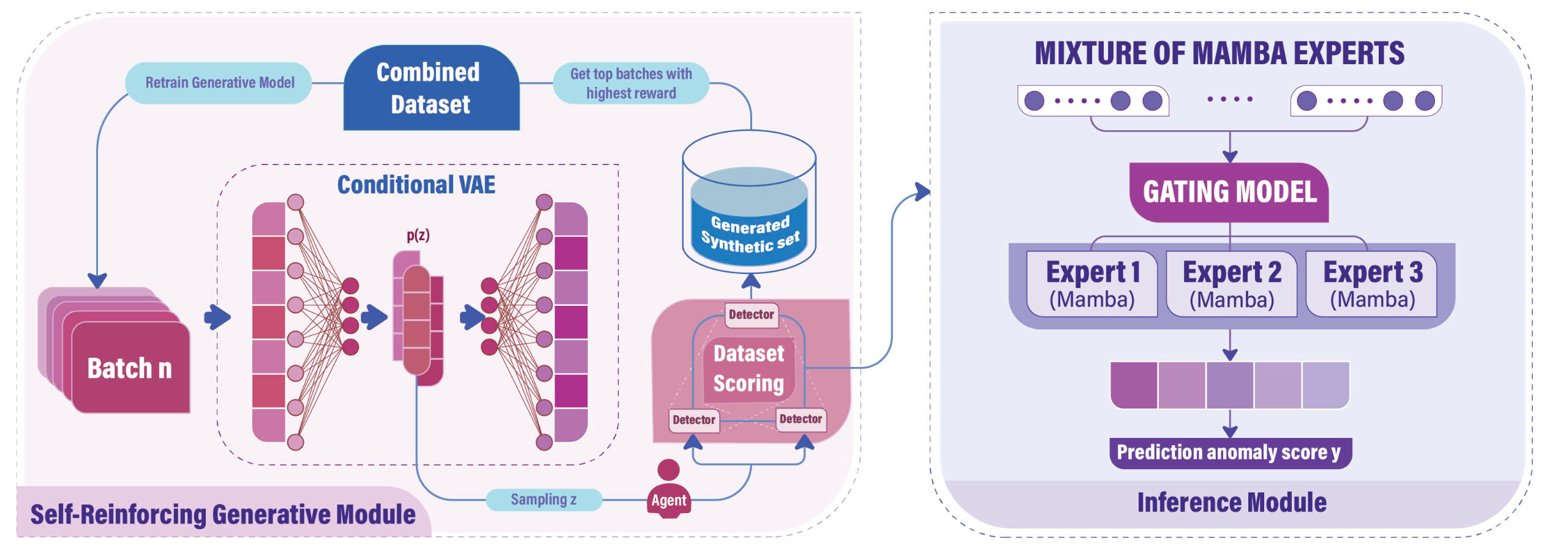
3.1 Self-Reinforcing Generative Module

This module includes two main models: a C-VAE generator, $\mathcal{F}_{\theta}$ , that synthesizes new anomalies, and a large Mamba-based detector $\mathcal{W}_{\kappa}:\mathbb{R}^{P}\rightarrow[0,1]$ parameterized by $\kappa$ that maps a sample $\bm{x}_{i}$ to a probabilistic score of it being an anomaly. Unlike conventional methods where the generator $\mathcal{F}_{\theta}$ relies solely on feedback from the detector $\mathcal{W}_{\kappa}$ to generate new samples which could lead to a model collapse (Salimans et al., 2016; Hassanaly et al., 2022) or vanishing gradient (Arjovsky & Bottou, 2017) problem, we instead leverage an RL agent to guide the training of $\mathcal{F}_{\theta}$ . This RL agent, represented by a policy $\pi_{\omega}$ , explores the latent distribution $p(z)$ of $\mathcal{F}_{\theta}$ and targets areas that would encourage the generator $\mathcal{F}_{\theta}$ to synthesize diverse and challenging anomalies that can bypass the detector $\mathcal{W}_{\kappa}$ . These synthetic samples are then used to augment the current training dataset and retrain $\mathcal{F}_{\theta}$ , ultimately improving its ability to generate better anomalies in future episodes.

Dataset definitions. The dataset $\mathcal{D}$ is split into a training set, $\mathcal{D}^{train}$ , and a testing set, $\mathcal{D}^{test}$ . In our approach, the goal is to attain high accuracy on the $\mathcal{D}^{test}$ even with a small training dataset $\mathcal{D}^{train}$ . Let $\mathcal{D}^{balanced}=\{(x,y)\in\mathcal{D}^{train}\mid j=\min(|\{y=-1\}|,|\{y=1\}|),|\{y=-1\}|=j,|\{y=1\}|=j\}$ be a dataset balanced between normal and anomalous data points, with equal cardinalities determined by the smaller class. Note that, as episodes progress, the generator $\mathcal{F}_{\theta}$ combined with the RL-agent $\pi_{\omega}$ adds more anomalous samples to $\mathcal{D}^{train}$ , expanding the anomalous data in $\mathcal{D}^{balanced}$ . Since $\mathcal{D}^{balanced}$ ensures equal numbers of anomalous and normal data, the increase in anomalous data leads to a corresponding expansion of normal data as well. In the RL context, for each episode, $e$ , we denote $\mathcal{D}^{train}_{e}$ and $\mathcal{D}^{balanced}_{e}$ as the evolving training and balanced datasets, respectively.

Training process. For each episode $e$ (comprising $h$ steps), the C-VAE generator $\mathcal{F}_{\theta}$ is trained with batches of $\mathcal{D}^{train}_{e}$ dataset, while the detector $\mathcal{W}_{\kappa}$ is trained with $\mathcal{D}^{balanced}_{e}$ . Next, an anomalous data point $(x,y=1)$ is sampled at random from $\mathcal{D}^{train}_{e,anomalous}$ , and converted into a latent representation $z=\mathcal{G}_{\psi}(x,y=1)$ . The RL policy is tasked with generating a modification vector $\delta$ in the latent space, i.e. $\pi_{\omega}:\bm{z}\rightarrow\delta$ . This $\delta$ results in a new sample in the latent space as $\hat{z}=z+\delta$ . At the end of the episode, a new dataset is obtained $\hat{\mathcal{X}}=\{\mathcal{M}_{\phi}(\hat{\bm{z}}_{0},y=1),\dots,\mathcal{M}_{\phi}(\hat{\bm{z}}_{h},y=1)\}$ . From the newly generated set $\hat{\mathcal{X}}$ , the top $l$ samples that lead to the highest rewards are selected and denoted as $\hat{\mathcal{X}}^{<l}$ . A formal definition of the reward is provided in the next section. At each episode, the selected samples are then merged with $\mathcal{D}^{train}_{e-1}$ , forming the evolving dataset $\mathcal{D}^{train}_{e}=\mathcal{D}^{train}_{e-1}\cup\hat{\mathcal{X}}^{<l}$ . Note that we set $\mathcal{D}_{0}=\mathcal{D}^{train}$ to ensure that the model $\mathcal{F}_{\theta}$ does not deviate from the acceptable range of the original data (Shumailov et al., 2024). The dataset $\mathcal{D}^{train}_{e}$ is used to retrain the generator $\mathcal{F}_{\theta}$ , enhancing its ability to generate high-quality data in future episodes. As $e$ increases, $\mathcal{D}^{train}_{e}$ is incorporated into $\mathcal{D}^{balanced}$ . Thus, $\mathcal{D}^{balanced}_{e}$ also grows across episodes. Due to page limit, we refer readers to Appendix A.1 for the pseudocode and further details about the training process.

3.1.1 Generating Samples as a Markov Decision Process

The process of policy modeling can be structured as a Markov Decision Process (MDP) (Bellman, 1957), $\mathcal{M}\stackrel{{\scriptstyle\text{ def }}}{{=}}(\mathcal{S},\mathcal{A},T,\mathcal{R})$ . This includes (i) a finite sets of states $\mathcal{S}$ , (ii) a finite set of actions $\mathcal{A}$ , (iii) a transition distribution $T(s^{\prime}\mid s,a)$ where $s,s^{\prime}\in\mathcal{S},a\in\mathcal{A}$ and (iv) a reward function $\mathcal{R}:\mathcal{S}\times\mathcal{A}\rightarrow\mathbb{R}$ . We specify each component as follows:

States $(s)$ : A state is defined by latent space representations $s_{i}=(\bm{z}_{i},\mathcal{D}^{train}_{e})$ for $\bm{z}_{i}=\mathcal{G}_{\psi}(\mathbf{x}_{i})$ and $\mathbf{x}_{i}\in\mathcal{D}^{train}_{e,anomalous}$ , where $\bm{z}_{i}$ is the latent vector produced by the encoder $\mathcal{G}_{\psi}$ from the input data $\mathbf{x}_{i}$ .

Actions ( $a)$ : An action $a_{i}=(\mu_{i},\sigma_{i})$ is a vector of two components: $\mu_{i}\in\mathbb{R}^{d}$ (predicted mean) and $\sigma_{i}\in\mathbb{R}^{d}$ (predicted scale). The modification vector $\delta_{i}=\sigma_{i}\cdot\epsilon+\mu_{i}$ , where $\epsilon\sim\mathcal{N}(0,I)$ , and the latent vector is updated as $\bm{\hat{z}}_{i}=\bm{z}_{i}+\delta_{i}$ .

Rewards ( $\mathcal{R}$ ): The reward function is strategically designed to encourage the generation of a set of samples that are diverse and reduce the detector’s confidence. The function is defined as follows:

\mathcal{R}(\mathcal{M}_{\phi}(\hat{z}_{i},y_{i}=1),e)=\gamma^{e}\cdot\mathcal{H}(\mathcal{D}^{train}_{e}\cup\mathcal{M}_{\phi}(\hat{z}_{i},y_{i}=1))-\log\mathcal{W}_{\kappa}(\mathcal{M}_{\phi}(\bm{\hat{z}}_{i},y_{i}=1)),

(3)

where $\mathcal{H}(\mathcal{D}^{train}_{e}\cup\mathcal{M}_{\phi}(\hat{z}_{i},y=1))$ is the entropy of $\mathcal{D}^{train}_{e}$ after incorporating $\mathcal{M}_{\phi}(\bm{\hat{z}}_{i},y_{i}=1)$ and is aimed at promoting the generation of diverse samples (additional details on the calculation of the entropy of $\mathcal{D}^{train}_{e}$ are provided in Appendix A.3). The function $\mathcal{W}_{\kappa}(\mathcal{M}_{\phi}(\bm{\hat{z}}_{i},y_{i}=1))$ assesses the detector’s likelihood of classifying the generated sample as anomalous, with the goal of reducing this probability to decrease the detector’s confidence.

The hyperparameter $\gamma\in[0,1]$ dictates the desired rate of entropy reduction. This $\gamma$ implies that the policy $\pi_{\omega}$ focuses on exploring rare samples to increase the diversity of $\mathcal{D}^{train}_{e,anomalous}$ in the early episodes. Once sufficient data has been explored, the reward function shifts to encourage the agent to exploit this data, generating new samples that are more effective at bypassing the detector.

Transition Dynamics ( $T$ ): When an action $a_{i}=(\mu_{i},\sigma_{i})$ is taken, a new anomalous data point $\hat{x}_{i}=\mathcal{M}_{\phi}(\bm{\hat{z}}_{i},y_{i}=1)$ is added to $\hat{\mathcal{X}}$ . A new state $s_{i+1}=(\bm{z}_{i+1},\mathcal{D}^{\text{train}}_{e})$ , where $\bm{z}_{i+1}=\mathcal{G}_{\psi}(\mathbf{x}_{i+1})$ , is then formed by selecting the next $x_{i+1}\in\mathcal{D}^{\text{train}}_{e,\text{anomalous}}$ .

3.1.2 One-step to Feasible Actions

The RL agent $\pi_{\omega}$ , which is tasked with generating a new sample $\hat{x}_{i}$ from $x_{i}$ , can be trained using conventional methods. However, during early training episodes, the agent would often struggle to find suitable actions that maximize the reward function because $\pi_{\omega}$ has not yet learned effective strategies. In fact, an action $a_{i}=(\mu_{i},\sigma_{i})$ may be invalid if the updated latent vector $\hat{z}_{i}$ derived from $a_{i}$ falls outside the supported range of the trained model $\mathcal{F}_{\theta}$ . Even with advanced exploration techniques such as those in (Eysenbach & Levine, 2022; Pathak et al., 2017; Burda et al., 2019; Ecoffet et al., 2021), this issue remains challenging for $\pi_{\omega}$ to overcome due to the high-dimensional and continuous nature of the action space.

A naive strategy to address this is to use the observed data distribution $p(x)$ (i.e., adding Gaussian noise to $x_{i}$ ) to generate new samples $\hat{x}_{i}$ . The encoder then provides their latent representation $\hat{z}_{i}=\mathcal{G}_{\psi}(\hat{x}_{i},y=1)$ , and the modification vector $\hat{\delta}_{i}=\hat{z}_{i}-z_{i}$ is employed to guide exploration at that step. After that, a feasible action $\tilde{a}_{i}=(\hat{\delta}_{i},\sigma_{i})$ is derived from $\hat{\delta}_{i}$ to replace the invalid action $a_{i}=(\mu_{i},\sigma_{i})$ of the RL agent in the current step. Once a feasible action is identified, the agent learns it in a supervised manner, facilitating more effective exploration in future steps. However, randomly modifying observations in the input space $p(x)$ can be complex. Instead, we rely on the following theorem to find feasible actions:

Theorem 1.

(Reward Estimation Consistency). If the reward function $\mathcal{R}$ is differentiable, $\mathcal{F}_{\theta}$ is well-converged, and $\hat{z}_{i}:=z_{i}-\epsilon\cdot\nabla_{z_{i}}(-\mathcal{R}(\mathcal{M}_{\phi}(\bm{z}_{i},y_{i}=1),e))$ for some small $\epsilon$ , then $\mathcal{R}\left(\hat{x}_{i},e\right)>\mathcal{R}\left(x_{i},e\right)$ , where $\hat{x}_{i}=\mathcal{M}_{\phi}(\hat{z}_{i},y_{i}=1)$ . (Proof in Appendix B.1)

In other words, if $\mathcal{F}_{\theta}$ is well-converged and maintains both continuity (i.e., nearby points in the latent space yield similar content when decoded) and completeness (i.e., points sampled from the latent space produce meaningful content when decoded), the C-VAE described in Equation 2 can explore new states $s$ (i.e., anomalous observations) by utilizing the latent feature space $p(z)$ (which is learned from the original space $p(\mathbf{x})$ ). This allows us to search for feasible $\hat{x}_{i}$ in the lower-dimensional and less noisy latent space $p(z)$ as an alternative to creating feasible actions. Specifically, Theorem 1 implies that we can deterministically search for $\hat{z}_{i}$ in a manner that maximizes the reward function specified in Equation 3 using gradient descent (Ruder, 2017).From that, a feasible action $\tilde{a}_{i}=(\hat{\delta}_{i},\sigma_{i})$ is derived where $\hat{\delta}_{i}=\hat{z}_{i}-z_{i}$ . With this approach, the policy, value, and reward models are trained simultaneously during these early episodes, allowing the RL agent to generalize effectively and reduce invalid actions in future episodes. Thus, the need for using one-step to feasible actions is eliminated in subsequent stages. Further details on this process can be found in Appendix A.2 with a preliminary analysis given in Appendix C.5.

3.2 Inference Module

At the conclusion of the first module, the detector $\mathcal{W}_{\kappa}$ has been augmented by the newly generated dataset and can be used as the final anomaly detection model. Due to the increasingly diverse training data generated by $\mathcal{F}_{\theta}$ , we had to initially overparameterize the detector $\mathcal{W}_{\kappa}$ . For that reason, deploying $\mathcal{W}_{\kappa}$ directly as the final detection model would not be scalable due to the high inference cost. Furthermore, the theorem below establishes a lower bound on the detection error, showing that any single detection model is subject to this lower bound regardless of the number of parameters.

Theorem 2.

(Inefficiency of single detector in handling evolving balance data). Suppose a feature space $\mathfrak{X}\subset\mathbb{R}^{P}$ contains $U_{n}$ normal clusters and $U_{a}$ anomalous clusters, where each cluster $u\text{-th}\in[U_{n}+U_{a}]$ is modeled as a Gaussian distribution $\mathcal{N}(\bm{\mu}_{u},\sigma^{2}\mathbf{I}_{P})$ . Let $\mathcal{V}_{\text{cluster}}$ be the cluster’s volume and $\Lambda$ be the total overlapping volume between normal and anomalous clusters, where the number of anomalous data points is equal to the number of normal data points, the training loss $\mathcal{L}_{\text{train }}\left(\mathcal{W}_{\kappa}\right)$ is lower bounded by $\frac{1}{4}\cdot\frac{\Lambda}{U_{a}\cdot V_{\text{cluster }}-\frac{\Lambda}{2}}$ in a case of linear $\mathcal{W}_{\kappa}$ . (Proof in Appendix B.2)

This theorem aligns with the findings in (Chen et al., 2022), emphasizing the inefficiency of using a single classifier. To address this issue, in this second module, we use the MoE approach to train an efficient detector on the dataset generated by the first module. Instead of relying on a single large-scale detector, this technique leverages multiple “expert” models, with each one specializing in a subset of the input data. The balanced dataset $\mathcal{D}^{balance}_{e}$ is first decomposed into clusters $\{\mathcal{C}_{1},\mathcal{C}_{2},\ldots,\mathcal{C}_{U}\}$ , where the number of clusters $U$ is determined using the elbow method (Yuan & Yang, 2019). We train a set of Mamba models $\{f_{1},f_{2},\dots,f_{M}\}$ , each acting as an expert for a specific data cluster following the Sparsely-Gated Mixture-of-Experts approach (Shazeer et al., 2017), and where $f_{m}(x;\mathbf{W})$ is the output of the $m$ -th expert network with input $x$ and parameter $\mathbf{W}$ .

Gating network. In the mixture-of-experts approach, the experts are complemented by a gating network that directs inputs to the most appropriate expert. Given an input $x\in\mathbb{R^{P}}$ , the gating network is defined as the following function:

\mathbf{h}(x,\aleph_{g},\aleph_{\text{noise}})=x\cdot\aleph_{\text{g}}+\text{StandardNormal}(.)\cdot\text{Softplus}\left(x\cdot\aleph_{\text{noise}}\right)

(4)

where $\aleph_{\text{g}},\aleph_{\text{noise}}\in\mathbb{R}^{P\times M}$ are weight matrices that determine the linear transformation and noise contribution, respectively. From the output of $\mathbf{h}(x,\aleph_{g},\aleph_{\text{noise}})$ , a key step is to apply the top $k$ expert selection mechanism, denoted by $\operatorname{TopK}(\mathbf{h}(x,\aleph_{g},\aleph_{\text{noise}}),k)$ , where it selects the top $k$ largest values from the vector $\mathbf{h}(x,\aleph_{g},\aleph_{\text{noise}})$ , which represents the performance scores (e.g., accuracy) of different expert networks. The elements in $\mathbf{h}(x,\aleph_{g},\aleph_{\text{noise}})$ that are not within the top $k$ are replaced by $-\infty$ , effectively excluding them from further consideration. Finally, a softmax function is applied to these top $k$ values to normalize them, i.e., $\lambda(x,\aleph_{g},\aleph_{\text{noise}})=\operatorname{Softmax}(\operatorname{TopK}(\mathbf{h}(x,\aleph_{g},\aleph_{\text{noise}}),k))$ . This setup forms a Mixture of Mamba Expert, and the output of the MoE layer is then expressed as:

\mathfrak{F}(x,\aleph_{g},\aleph_{\text{noise}},\mathbf{W})=\sum_{m\in\mathfrak{T}_{x}}\lambda_{m}(x,\aleph_{g},\aleph_{\text{noise}})f_{m}(x;\mathbf{W})

(5)

where $\mathfrak{T}_{\mathbf{x}}\subseteq[M]$ represents the indices of selected experts ( $|\mathfrak{T}_{\mathbf{x}}|=k$ ).

Tackling “winner-take-all”. During early training of MoE, experts have arbitrary performance scores, hence the gating network could randomly allocate more samples to a particular expert. With more training data, this expert outperforms others, thus receiving even more samples. This is referred to as the ”winner-take-all” phenomenon (Oster & Liu, 2005; Fedus et al., 2022), which reduces the MoE to a single lightweight expert, limiting its ability to generalize. While this expert may excel, it fails to capture the diverse features across $U$ clusters, undermining the model’s overall performance.

We tackle this “winner-take-all” issue by temporarily deactivating the gating network during this early training stage and, instead, proposing a probabilistic approach to ensure diversity in cluster assignments across experts, while also considering the complexity of each cluster. For each expert $f_{i}$ , where $i\in[M]$ , instead of assigning clusters based on fixed criteria, we dynamically adjust the probability of an expert $f_{i}$ selecting a cluster $u_{i}\in[U]$ , with the probability inversely proportional to how frequently the cluster has already been assigned to other experts. More importantly, we introduce a scaling factor that adjusts this probability based on the size of the cluster. For larger clusters, which are likely more complex, we reduce the penalty of being selected multiple times, as these clusters require more experts to fully capture their complexity. Specifically, the probability of expert $f_{i}$ selecting cluster $u$ is given by:

\mathcal{P}(u\mid\mathbf{x},\{n_{u}\},\{s_{u}\})=\frac{\exp\left(c_{0}-\frac{\alpha}{s_{u}}\cdot n_{u}\right)}{\sum_{u^{\prime}\in[U]}\exp\left(c_{0}-\frac{\alpha}{s_{u^{\prime}}}\cdot n_{u^{\prime}}\right)}

(6)

where $s_{u}$ is the size of cluster $u$ , $n_{u}$ is the number of times cluster $u$ has already been assigned, $\alpha$ is the base penalty factor, and $c_{0}$ is a constant initialization score for cluster selection. Then, the expert $f_{i}$ will select $u\sim\operatorname{Categorical}\left(\mathcal{P}\left(u\mid\mathbf{x},\left\{n_{u}\right\},\left\{s_{u}\right\}\right),u\in[U]\right)$ as its cluster.

Note that, due to the probabilistic nature of the selection algorithm, there could be clusters that are not selected by any experts. Therefore, we overspecify the number of experts $M$ . As demonstrated in a theorem from (Nguyen et al., 2024), doing so does not increase prediction time. This is because $\mathfrak{F}(x,\aleph_{g},\aleph_{\text{noise}},\mathbf{W})$ selects only the top $k$ (typically 2 or 3) best experts for making predictions. After training each expert with its selected cluster, we train the gating network to minimize the overall classification loss (e.g., MSE or Cross Entropy Loss). With this setup, we also establish a theorem to demonstrate the effectiveness of our training mechanism as follows:

Theorem 3.

(MoME efficiently handles evolving balance data). Let $\mathcal{L}_{test}(\mathfrak{F})$ and $\mathcal{L}_{test}(\mathcal{W}_{\kappa})$ represent the expected error on the test set for the Mixture of Mamba Experts (MoME) model and a single detector, respectively. For any value of $\Lambda$ , employing MoME with $\{f_{1},f_{2},\dots,f_{M}\}$ guarantees that the minimum expected error on the training set is $\mathcal{L}_{train}(\mathfrak{F})=0$ and the expected error on the test set satisfies $\mathcal{L}_{test}(\mathfrak{F})\leq\mathcal{L}_{test}(\mathcal{W}_{\kappa})$ . (Proof in Appendix B.3)

The above theorem demonstrates that a Mixture of Mamba Experts model can effectively fit all the data in the training set. Moreover, the expected error on the test set when using the Mixture of Mamba Experts will always be less than or equal to that of a single detector. Once the experts are well-trained, we activate the gating network and use it for routing samples.

4 Experimental Evaluation

Settings. We conduct experiments to evaluate the performance of our Swift Hydra framework using the ADBench benchmark (Han et al., 2022), which includes a comprehensive collection of 57 widely used anomaly detection datasets spanning various tasks, from image analysis to natural language processing, as detailed in Appendix C.6. We also evaluate a version of Swift Hydra without MoME, i.e., a single large detector is used in the Inference Module. The implementation specifics, such as the training algorithm, model architecture, hyperparameter, model size, and training costs are provided in Appendix C.1. For the RL training, we use Proximal Policy Optimization (Do et al., 2024; Schulman et al., 2017; Do et al., 2021; Ngo et al., 2024; Khoi et al., 2021) as it is a simple yet effective algorithm. We will release the source code once the paper is published.

Metrics. In our evaluation, we focus on the performance of the Swift Hydra, particularly in terms of AUC-ROC and TIF (total inference time to predict all data in ADBench). Additionally, we analyze the distribution of generated data at each episode and compare it to the distribution of the test data.

Baselines. For the anomaly detection task, we compare Swift Hydra against several state-of-the-art (SOTA) semi-supervised and unsupervised learning methods included in ADBench. These methods are Rejex (Perini & Davis, 2023), ADGym (Jiang et al., 2023) and DTE (Livernoche et al., 2024). We also compare the distribution of our generated data against that of data generated by oversampling techniques such as SMOTE (Chawla et al., 2002), Borderline-SMOTE (Han et al., 2005), ADASYN (He et al., 2008), SVM-SMOTE (Nguyen et al., 2011), CBO (Xu et al., 2021), Oversampling GAN (Nazari & Branco, 2021) and VAE-Geometry (Chadebec et al., 2023). For each method, we use the best-performing hyperparameters as provided in its original paper.

Methods	DTE		Rejex		ADGym		Swift Hydra (Single)		Swift Hydra (MoME)
	AUCROC	TIF	AUCROC	TIF	AUCROC	TIF	AUCROC	TIF	AUCROC	TIF
Train/Test Ratio (40/60%)	0.82	4.02	0.78	3.89	0.86	6.12	0.91	13.11	0.93	4.01
Train/Test Ratio (30/70%)	0.80	4.13	0.77	4.09	0.82	7.03	0.90	14.38	0.91	4.79
Train/Test Ratio (20/80%)	0.79	4.31	0.76	4.22	0.79	8.17	0.87	16.13	0.90	5.22
Train/Test Ratio (10/90%)	0.78	4.42	0.74	4.39	0.77	9.14	0.86	18.52	0.87	5.84
TIF = Total Inference Time (Seconds)

Table 1: The performance of Swift Hydra and the baselines on the ADBench is evaluated based on two criteria: AUC-ROC and total inference time (TIF). Here, the AUC-ROC is the average calculated across all 57 datasets, while the TIF represents the total time the model takes to predict all data points across all datasets. We vary the train/test ratios to illustrate how the size of the training data impacts the performance. The best AUC-ROC values are highlighted.

AUC-ROC Evaluation. As shown in Table 1, the average AUC-ROC scores show that both versions of Swift Hydra - single large detector and MoME - consistently outperform other state-of-the-art (SOTA) methods with respect to various training sizes (i.e., 40%, 30%, 20%, and 10% of the whole dataset). Notably, with only 10% of the dataset, Swift Hydra outperforms DTE in the semi-supervised setting and Rejex in the unsupervised setting. This demonstrates that our RL algorithm can train a generative model to synthesize effective anomalies that can later be used to train a high-performing detection model. We refer readers to Appendix C.2 for a comparative analysis with more SOTA detection methods and oversampling techniques, and Appendix C.3 for a toy example to illustrate the generalization ability of Swift Hydra. Appendix C.4 presents a series of ablation studies evaluating the impact of the Self-Reinforcing Module, the effectiveness of the probabilistic cluster assignments (as described in Equation 6), and the influence of the KL term and the reconstruction term in Equation 2 on the AUC-ROC of Swift Hydra.

Inference Time Evaluation. In terms of total inference time across 57 datasets, Table 1 shows that Rejex has the shortest time, which is expected as it relies on conventional lazy learning methods such as Isolation Forest. DTE, which is based on a diffusion model, requires only a few steps to reconstruct backward and determine whether a sample is anomalous, resulting in relatively short inference times. Although ADGym optimally selects which ML models to use for each dataset, the experiment shows that its overall prediction time is still relatively high compared to that of Swift Hydra (MoME). Swift Hydra (Single) achieves high AUC-ROC scores; nevertheless, its prediction time is significantly longer because a single large model is designed to capture the entire diverse dataset generated by the Self-Reinforcing Generative Module. In contrast, Swift Hydra (MoME) not only attains the best AUC-ROC scores but also has efficient prediction times that are comparable to DTE with respect to the training sizes of 40% and 30%. Overall, Swift Hydra (MoME) offers the best balance between AUC-ROC performance and inference time among the tested methods.

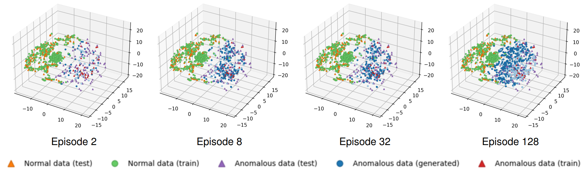
Generated Data Distribution. We visualize the distribution of data generated over time by our Self-Reinforcing Generative Module in Figure 2. Initially, the model explores a broad spectrum of widely dispersed anomalous data points. As the episodes progress, a discernible pattern emerges: the generated anamalous points increasingly cluster towards the boundary that separates normal from anomalous data. In fact, this transitional zone at the boundary highlights the anomalies that are not easily distinguishable from normal data points. Hence, this dynamic progression shows that our generative method significantly enriches the diversity of anomalous data points while simultaneously pushing for the most challenging anomalies, thus strengthening the detector’s generalization ability.

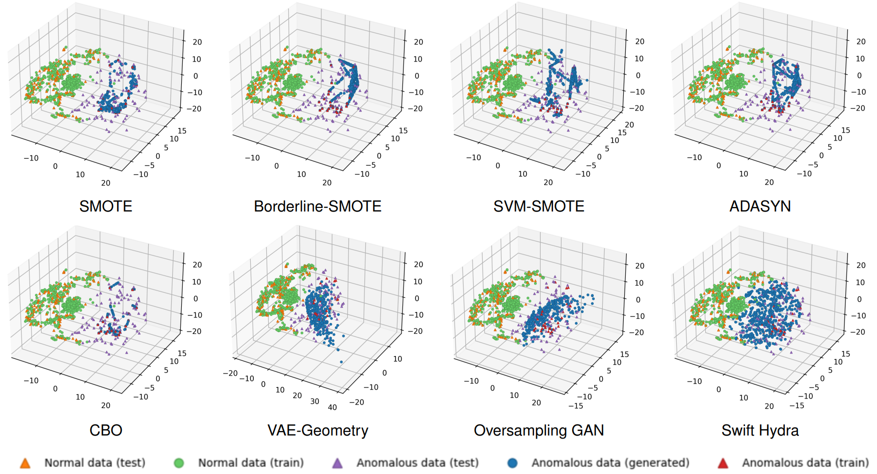
Figure 3 shows a comparative analysis on the generated data distribution of our method and that of other oversampling methods. As can be seen, methods like SMOTE, Borderline-SMOTE, SVM-SMOTE, ADASYN, and CBO only generate data points within the boundary of the anomalous data in the training set, while our approach allows data points to be generated beyond these boundaries. This enables our method to potentially generate anomalous data points that can cover the distribution of the test set. Although VAE-Geometry and Oversampling GAN also explore beyond the boundary, they have limitations. Oversampling GAN suffers from model collapse (Salimans et al., 2016; Hassanaly et al., 2022): during the early training steps, if it finds one data point that is very good at fooling the detector, it will only focus on generating samples around that point in subsequent steps. VAE-Geometry performs better as it generates more diverse data points. However, it is highly sensitive to hyperparameters to learn the data manifold correctly, hence, it is less effective compared to our method. Both Figures 2 and 3 demonstrate that data generated by Swift Hydra provides comprehensive coverage over the range of anomalous data in the test set, even though no knowledge about the test data is provided during training.

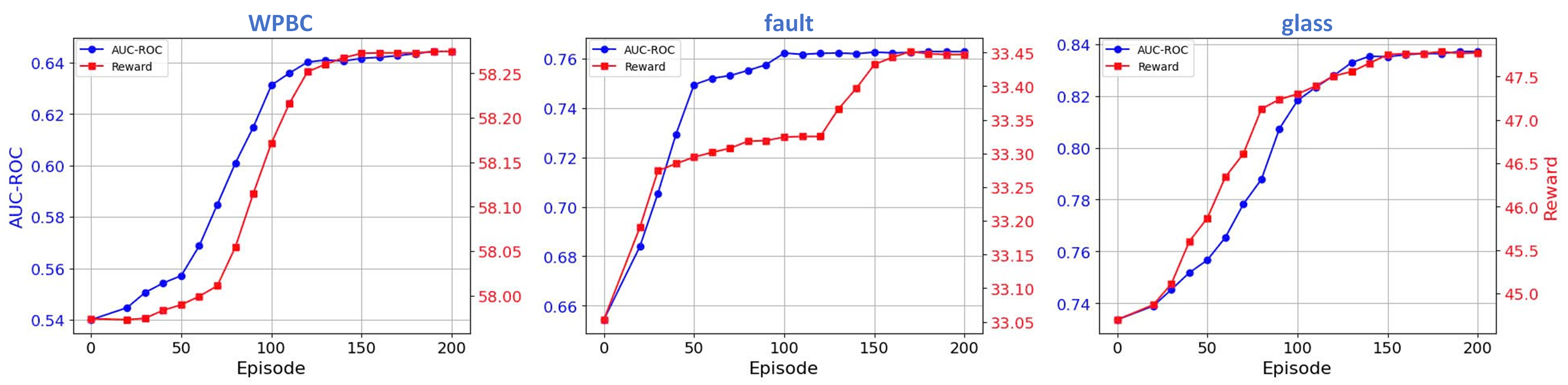
Soundness of the Reward Function. Figure 4 shows that the reward trend (average of multiple roll-outs) closely follows the increase in AUC-ROC. This demonstrates the soundness of our reward function, as the RL agent optimizes the reward function, either by predicting actions itself or using feasible actions as discussed in Section 3.1.2, leading to the maximization of AUC-ROC in the test set. Interestingly, even though the RL agent receives no feedback on how it performs on the test set (no knowledge about the test set is provided during training), it still manages to increase the AUC-ROC over time. This suggests that our reward function helps improve the detector’s generalization ability.

5 Related Work

Anomaly Detection. Due to the high cost and difficulty of data annotation, most recent anomaly detection (AD) research has focused on unsupervised methods with various data distribution assumptions (Aggarwal, 2017; Liu et al., 2008; Zong et al., 2018; Li et al., 2020; 2022; Xu et al., 2022). Common approaches like GAN-based (Donahue et al., 2017; Schlegl et al., 2017), self-supervised (Hojjati et al., 2022; Sehwag et al., 2021; Georgescu et al., 2021; Li et al., 2021), and one-class classification (Shen et al., 2020; Hu et al., 2020) typically rely solely on normal data for training, making it difficult to identify anomalies due to the absence of true anomaly patterns. Reconstruction-based methods (An & Cho, 2015; Xu et al., 2022) use anomaly reconstruction loss to detect outliers but are often unreliable as neural networks can memorize and generalize even with a few samples of anomalies. More recent supervised or weakly-supervised methods (Pang et al., 2018b; 2019a; 2019d; Ruff et al., 2020; Zhou et al., 2021) treat anomalies as negative samples to improve sensitivity, but they risk overfitting and heavily depend on the diversity and quality of the dataset.

Advanced methods like ADGym (Jiang et al., 2023) have improved anomaly detection through optimized data processing, augmentation, network design, and training, but they may fail if settings do not align with the target domain. Learning to Reject (Perini & Davis, 2023) uses uncertainty scores to reject rather than forcibly predict uncertain samples; however, it often rejects data near the normal-anomaly boundary, reducing detection performance. DTE (Livernoche et al., 2024) leverages diffusion models to estimate posterior densities, but the decoder can still memorize and reconstruct anomalies, complicating reliable scoring. AnomalyClip (Zhou et al., 2024) captures general anomalies in images using object-agnostic text prompts but is limited to image-based tasks.

Oversampling-based techniques. Traditional oversampling techniques tackle imbalanced data by generating synthetic samples. SMOTE (Chawla et al., 2002) interpolates between minority points to increase diversity but does not focus on challenging samples. Variations like CBO (Xu et al., 2021), Borderline-SMOTE (Han et al., 2005), and SVM-SMOTE (Nguyen et al., 2011) generate samples near boundaries to improve representation but risk introducing noise and overfitting in complex distributions. ADASYN (He et al., 2008) targets harder instances for sample generation, enhancing performance but potentially causing redundancy if not carefully managed.

Recent techniques like Oversampling GAN (Nazari & Branco, 2021) and VAE-Geometry (Chadebec et al., 2023) use deep learning to generate more generalized samples. Oversampling GAN may suffer from issues like vanishing gradients or model collapse, limiting sample diversity. VAE-Geometry employs a Variational Autoencoder that preserves the geometric structure of the data during augmentation, producing synthetic samples that more accurately reflect the true distribution. However, its accuracy depends on correctly learning the data manifold and is highly sensitive to hyperparameters; failure to capture complex structures can result in inaccurate sample generation.

RL-Guided Generative AI. Reinforcement Learning (RL) has been used to guide Generative AI (GenAI) in large language models (LLMs), as seen in ”Learning from Human Feedback” (Dubois et al., 2023) and ReST (Gulcehre et al., 2023), enhancing generative capabilities through reward models. The direct use of RL to guide the sample generation process of generative models in anomaly detection remains underexplored, with this approach only recently gaining traction through the ReST framework for LLMs.

6 Conclusion

We propose Swift Hydra, a framework designed to reinforce a generative model’s ability to synthesize anomalies in order to augment anomaly detection models. The framework features an RL agent to guide the training of a C-VAE model that generates diverse and challenging anomalies. We further propose a mechanism to help the RL agent choose an action more efficiently during training. Additionally, due to the diverse nature of the generated dataset, we introduce a Mixture of Mamba Experts to train an efficient anomaly detector, where each expert specializes in capturing specific data clusters. As a result, our model demonstrates strong generalization capabilities and fast inference, as evidenced by experiments conducted on the ADBench benchmark against state-of-the-art anomaly detection models. Our research highlights a promising paradigm of integrating RL and generative AI for advancing anomaly detection. It can also be leveraged for generating and synthesizing data in other application contexts where collecting real data is expensive and scarce.

Acknowledgments

This work was partially supported by the National Science Foundation under the SaCT program, grant number CNS-1935923, and by the Korea Institute of Energy Technology Evaluation and Planning (KETEP) grant funded by the Korea government (MOTIE) (RS-2023-00303559, Study on developing cyber-physical attack response system and security management system to maximize real-time distributed resource availability).

This work was authored in part by the National Renewable Energy Laboratory, operated by Alliance for Sustainable Energy, LLC, for the U.S. Department of Energy (DOE) under Contract No. DE-AC36-08GO28308. Funding provided by the U.S. Department of Energy Office of Cybersecurity, Energy Security, and Emergency Response (CESER), and by the Laboratory Directed Research and Development (LDRD) Program at NREL. The views expressed in the article do not necessarily represent the views of the DOE or the U.S. Government. The U.S. Government retains and the publisher, by accepting the article for publication, acknowledges that the U.S. Government retains a nonexclusive, paid-up, irrevocable, worldwide license to publish or reproduce the published form of this work, or allow others to do so, for U.S. Government purposes.

References

Aggarwal (2017) Charu C Aggarwal. An introduction to outlier analysis. In Outlier analysis, pp. 1–34. Springer, 2017.
An & Cho (2015) Jinwon An and Sungzoon Cho. Variational autoencoder based anomaly detection using reconstruction probability. 2015. URL https://api.semanticscholar.org/CorpusID:36663713.
Arjovsky & Bottou (2017) Martin Arjovsky and Leon Bottou. Towards principled methods for training generative adversarial networks. In International Conference on Learning Representations, 2017. URL https://openreview.net/forum?id=Hk4_qw5xe.
Bellman (1957) Richard Bellman. A markovian decision process. Journal of mathematics and mechanics, pp. 679–684, 1957.
Burda et al. (2019) Yuri Burda, Harrison Edwards, Amos Storkey, and Oleg Klimov. Exploration by random network distillation. In International Conference on Learning Representations, 2019. URL https://openreview.net/forum?id=H1lJJnR5Ym.
Chadebec et al. (2023) Clément Chadebec, Elina Thibeau-Sutre, Ninon Burgos, and Stéphanie Allassonnière. Data augmentation in high dimensional low sample size setting using a geometry-based variational autoencoder. IEEE Transactions on Pattern Analysis and Machine Intelligence, 45(3):2879–2896, 2023. doi: 10.1109/TPAMI.2022.3185773.
Chawla et al. (2002) Nitesh V Chawla, Kevin W Bowyer, Lawrence O Hall, and W Philip Kegelmeyer. Smote: synthetic minority over-sampling technique. Journal of artificial intelligence research, 16:321–357, 2002.
Chen et al. (2022) Zixiang Chen, Yihe Deng, Yue Wu, Quanquan Gu, and Yuanzhi Li. Towards understanding the mixture-of-experts layer in deep learning. In S. Koyejo, S. Mohamed, A. Agarwal, D. Belgrave, K. Cho, and A. Oh (eds.), Advances in Neural Information Processing Systems, volume 35, pp. 23049–23062. Curran Associates, Inc., 2022. URL https://proceedings.neurips.cc/paper_files/paper/2022/file/91edff07232fb1b55a505a9e9f6c0ff3-Paper-Conference.pdf.
Child (2021) Rewon Child. Very deep {vae}s generalize autoregressive models and can outperform them on images. In International Conference on Learning Representations, 2021. URL https://openreview.net/forum?id=RLRXCV6DbEJ.
Do et al. (2021) Nguyen Do, Dung Truong, Duy Nguyen, Minh Hoai, and Cuong Pham. Self-controlling photonic-on-chip networks with deep reinforcement learning. Scientific Reports, 11(1):23151, Nov 2021. ISSN 2045-2322. doi: 10.1038/s41598-021-02583-7. URL https://doi.org/10.1038/s41598-021-02583-7.
Do et al. (2024) Nguyen Do, Tanmoy Chowdhury, Chen Ling, Liang Zhao, and My T. Thai. Mim-reasoner: Learning with theoretical guarantees for multiplex influence maximization, 2024. URL https://arxiv.org/abs/2402.16898.
Donahue et al. (2017) Jeff Donahue, Philipp Krähenbühl, and Trevor Darrell. Adversarial feature learning, 2017. URL https://arxiv.org/abs/1605.09782.
Dubois et al. (2023) Yann Dubois, Xuechen Li, Rohan Taori, Tianyi Zhang, Ishaan Gulrajani, Jimmy Ba, Carlos Guestrin, Percy Liang, and Tatsunori Hashimoto. Alpacafarm: A simulation framework for methods that learn from human feedback. In Thirty-seventh Conference on Neural Information Processing Systems, 2023. URL https://openreview.net/forum?id=4hturzLcKX.
Ecoffet et al. (2021) Adrien Ecoffet, Joost Huizinga, Joel Lehman, Kenneth O. Stanley, and Jeff Clune. First return, then explore. Nature, 590(7847):580–586, Feb 2021. ISSN 1476-4687. doi: 10.1038/s41586-020-03157-9. URL https://doi.org/10.1038/s41586-020-03157-9.
Eysenbach & Levine (2022) Benjamin Eysenbach and Sergey Levine. Maximum entropy RL (provably) solves some robust RL problems. In International Conference on Learning Representations, 2022. URL https://openreview.net/forum?id=PtSAD3caaA2.
Fedus et al. (2022) William Fedus, Barret Zoph, and Noam Shazeer. Switch transformers: scaling to trillion parameter models with simple and efficient sparsity. J. Mach. Learn. Res., 23(1), jan 2022. ISSN 1532-4435.
Georgescu et al. (2021) Mariana-Iuliana Georgescu, Antonio Barbalau, Radu Tudor Ionescu, Fahad Shahbaz Khan, Marius Popescu, and Mubarak Shah. Anomaly detection in video via self-supervised and multi-task learning. In Proceedings of the IEEE/CVF conference on computer vision and pattern recognition, pp. 12742–12752, 2021.
Goodfellow et al. (2016) Ian Goodfellow, Yoshua Bengio, Aaron Courville, and Yoshua Bengio. Deep learning, volume 1. MIT Press, 2016.
Gorishniy et al. (2023) Yury Gorishniy, Ivan Rubachev, Valentin Khrulkov, and Artem Babenko. Revisiting deep learning models for tabular data, 2023. URL https://arxiv.org/abs/2106.11959.
Görnitz et al. (2013) Nico Görnitz, Marius Kloft, Konrad Rieck, and Ulf Brefeld. Toward supervised anomaly detection. Journal of Artificial Intelligence Research, 46:235–262, 2013.
Gu & Dao (2024) Albert Gu and Tri Dao. Mamba: Linear-time sequence modeling with selective state spaces, 2024. URL https://arxiv.org/abs/2312.00752.
Gulcehre et al. (2023) Caglar Gulcehre, Tom Le Paine, Srivatsan Srinivasan, Ksenia Konyushkova, Lotte Weerts, Abhishek Sharma, Aditya Siddhant, Alex Ahern, Miaosen Wang, Chenjie Gu, Wolfgang Macherey, Arnaud Doucet, Orhan Firat, and Nando de Freitas. Reinforced self-training (rest) for language modeling, 2023. URL https://arxiv.org/abs/2308.08998.
Han et al. (2005) Hui Han, Wen-Yuan Wang, and Bing-Huan Mao. Borderline-smote: a new over-sampling method in imbalanced data sets learning. In International conference on intelligent computing, pp. 878–887. Springer, 2005.
Han et al. (2022) Songqiao Han, Xiyang Hu, Hailiang Huang, Minqi Jiang, and Yue Zhao. ADBench: Anomaly detection benchmark. Advances in Neural Information Processing Systems (NeurIPS), 35:32142–32159, 2022.
Hassanaly et al. (2022) Malik Hassanaly, Andrew Glaws, Karen Stengel, and Ryan N King. Adversarial sampling of unknown and high-dimensional conditional distributions. Journal of Computational Physics, 450:110853, 2022.
He et al. (2008) Haibo He, Yang Bai, Edwardo A. Garcia, and Shutao Li. Adasyn: Adaptive synthetic sampling approach for imbalanced learning. In 2008 IEEE International Joint Conference on Neural Networks (IEEE World Congress on Computational Intelligence), pp. 1322–1328, 2008. doi: 10.1109/IJCNN.2008.4633969.
Hojjati et al. (2022) Hadi Hojjati, Thi Kieu Khanh Ho, and Narges Armanfard. Self-supervised anomaly detection: A survey and outlook. arXiv preprint arXiv:2205.05173, 2022.
Hu et al. (2020) Wenpeng Hu, Mengyu Wang, Qi Qin, Jinwen Ma, and Bing Liu. Hrn: A holistic approach to one class learning. In H. Larochelle, M. Ranzato, R. Hadsell, M.F. Balcan, and H. Lin (eds.), Advances in Neural Information Processing Systems, volume 33, pp. 19111–19124. Curran Associates, Inc., 2020. URL https://proceedings.neurips.cc/paper_files/paper/2020/file/dd1970fb03877a235d530476eb727dab-Paper.pdf.
Jiang et al. (2023) Minqi Jiang, Chaochuan Hou, Ao Zheng, Songqiao Han, Hailiang Huang, Qingsong Wen, Xiyang Hu, and Yue Zhao. Adgym: Design choices for deep anomaly detection, 2023. URL https://arxiv.org/abs/2309.15376.
Khoi et al. (2021) Nguyen Khoi, Cuong Van, Hoang Tran, and Cao Dung Truong. Multi-objective exploration for proximal policy optimization. pp. 105–109, 03 2021. doi: 10.1109/ATiGB50996.2021.9423319.
Kingma & Welling (2013) Diederik P Kingma and Max Welling. Auto-encoding variational bayes. arXiv preprint arXiv:1312.6114, 2013.
Leibig et al. (2017) Christian Leibig, Vaneeda Allken, Murat Seçkin Ayhan, Philipp Berens, and Siegfried Wahl. Leveraging uncertainty information from deep neural networks for disease detection. Scientific reports, 7(1):1–14, 2017.
Li et al. (2021) Chun-Liang Li, Kihyuk Sohn, Jinsung Yoon, and Tomas Pfister. Cutpaste: Self-supervised learning for anomaly detection and localization. In Proceedings of the IEEE/CVF Conference on Computer Vision and Pattern Recognition, pp. 9664–9674, 2021.
Li et al. (2020) Zheng Li, Yue Zhao, Nicola Botta, Cezar Ionescu, and Xiyang Hu. Copod: copula-based outlier detection. In 2020 IEEE international conference on data mining (ICDM), pp. 1118–1123. IEEE, 2020.
Li et al. (2022) Zheng Li, Yue Zhao, Xiyang Hu, Nicola Botta, Cezar Ionescu, and George Chen. Ecod: Unsupervised outlier detection using empirical cumulative distribution functions. IEEE Transactions on Knowledge and Data Engineering, 2022.
Liao et al. (2013) Hung-Jen Liao, Chun-Hung Richard Lin, Ying-Chih Lin, and Kuang-Yuan Tung. Intrusion detection system: A comprehensive review. Journal of Network and Computer Applications, 36(1):16–24, 2013.
Liu et al. (2008) Fei Tony Liu, Kai Ming Ting, and Zhi-Hua Zhou. Isolation forest. In 2008 eighth ieee international conference on data mining, pp. 413–422. IEEE, 2008.
Liu et al. (2019) Wen Liu, Weixin Luo, Zhengxin Li, Peilin Zhao, Shenghua Gao, et al. Margin learning embedded prediction for video anomaly detection with a few anomalies. In IJCAI, volume 3, pp. 023–3, 2019.
Livernoche et al. (2024) Victor Livernoche, Vineet Jain, Yashar Hezaveh, and Siamak Ravanbakhsh. On diffusion modeling for anomaly detection. In The Twelfth International Conference on Learning Representations, 2024. URL https://openreview.net/forum?id=lR3rk7ysXz.
Nazari & Branco (2021) Ehsan Nazari and Paula Branco. On oversampling via generative adversarial networks under different data difficulty factors. In Nuno Moniz, Paula Branco, Luis Torgo, Nathalie Japkowicz, Michał Woźniak, and Shuo Wang (eds.), Proceedings of the Third International Workshop on Learning with Imbalanced Domains: Theory and Applications, volume 154 of Proceedings of Machine Learning Research, pp. 76–89. PMLR, 17 Sep 2021. URL https://proceedings.mlr.press/v154/nazari21a.html.
Ngo et al. (2024) Hoang M. Ngo, Nguyen H K. Do, Minh N. Vu, Tamer Kahveci, and My T. Thai. Charme: A chain-based reinforcement learning approach for the minor embedding problem, 2024. URL https://arxiv.org/abs/2406.07124.
Nguyen et al. (2011) Hien M. Nguyen, Eric W. Cooper, and Katsuari Kamei. Borderline over-sampling for imbalanced data classification. Int. J. Knowl. Eng. Soft Data Paradigm., 3(1):4–21, April 2011. ISSN 1755-3210. doi: 10.1504/IJKESDP.2011.039875. URL https://doi.org/10.1504/IJKESDP.2011.039875.
Nguyen et al. (2024) Huy Nguyen, Pedram Akbarian, Fanqi Yan, and Nhat Ho. Statistical perspective of top-k sparse softmax gating mixture of experts. In The Twelfth International Conference on Learning Representations, 2024. URL https://openreview.net/forum?id=jvtmdK69KQ.
Oster & Liu (2005) Matthias Oster and Shih-Chii Liu. Spiking inputs to a winner-take-all network. In Y. Weiss, B. Schölkopf, and J. Platt (eds.), Advances in Neural Information Processing Systems, volume 18. MIT Press, 2005. URL https://proceedings.neurips.cc/paper_files/paper/2005/file/881c6efa917cff1c97a74e03e15f43e8-Paper.pdf.
Pang et al. (2018a) Guansong Pang, Longbing Cao, Ling Chen, and Huan Liu. Learning representations of ultrahigh-dimensional data for random distance-based outlier detection. In Proceedings of the 24th ACM SIGKDD International Conference on Knowledge Discovery & Data Mining, KDD ’18, pp. 2041–2050, New York, NY, USA, 2018a. Association for Computing Machinery. ISBN 9781450355520. doi: 10.1145/3219819.3220042. URL https://doi.org/10.1145/3219819.3220042.
Pang et al. (2018b) Guansong Pang, Longbing Cao, Ling Chen, and Huan Liu. Learning representations of ultrahigh-dimensional data for random distance-based outlier detection. In KDD, pp. 2041–2050, 2018b.
Pang et al. (2019a) Guansong Pang, Chunhua Shen, Huidong Jin, and Anton van den Hengel. Deep weakly-supervised anomaly detection. ArXiv, 1910.13601, 2019a. URL https://arxiv.org/abs/1910.13601.
Pang et al. (2019b) Guansong Pang, Chunhua Shen, and Anton van den Hengel. Deep anomaly detection with deviation networks, 2019b. URL https://arxiv.org/abs/1911.08623.
Pang et al. (2019c) Guansong Pang, Chunhua Shen, and Anton Van Den Hengel. Deep anomaly detection with deviation networks. In Proceedings of the 25th ACM SIGKDD international conference on knowledge discovery & data mining, pp. 353–362, 2019c.
Pang et al. (2019d) Guansong Pang, Chunhua Shen, and Anton van den Hengel. Deep anomaly detection with deviation networks. In KDD, pp. 353–362, 2019d.
Pang et al. (2021) Guansong Pang, Choubo Ding, Chunhua Shen, and Anton van den Hengel. Explainable deep few-shot anomaly detection with deviation networks. arXiv preprint arXiv:2108.00462, 2021.
Pathak et al. (2017) Deepak Pathak, Pulkit Agrawal, Alexei A. Efros, and Trevor Darrell. Curiosity-driven exploration by self-supervised prediction. In 2017 IEEE Conference on Computer Vision and Pattern Recognition Workshops (CVPRW), pp. 488–489, 2017. doi: 10.1109/CVPRW.2017.70.
Perini & Davis (2023) Lorenzo Perini and Jesse Davis. Unsupervised anomaly detection with rejection, 2023. URL https://arxiv.org/abs/2305.13189.
Ruder (2017) Sebastian Ruder. An overview of gradient descent optimization algorithms, 2017. URL https://arxiv.org/abs/1609.04747.
Ruff et al. (2020) Lukas Ruff, Robert A. Vandermeulen, Nico Görnitz, Alexander Binder, Emmanuel Müller, Klaus-Robert Müller, and Marius Kloft. Deep semi-supervised anomaly detection. In ICLR. OpenReview.net, 2020.
Sahu et al. (2024) Abhijeet Sahu, Truc Nguyen, Kejun Chen, Xiangyu Zhang, and Malik Hassanaly. Detection of false data injection attacks (fdia) on power dynamical systems with a state prediction method. IEEE Access, 2024.
Salimans et al. (2016) Tim Salimans, Ian Goodfellow, Wojciech Zaremba, Vicki Cheung, Alec Radford, and Xi Chen. Improved techniques for training GANs. In Advances in neural information processing systems, pp. 2234–2242, 2016.
Schlegl et al. (2017) Thomas Schlegl, Philipp Seeböck, Sebastian M. Waldstein, Ursula Schmidt-Erfurth, and Georg Langs. Unsupervised anomaly detection with generative adversarial networks to guide marker discovery, 2017. URL https://arxiv.org/abs/1703.05921.
Schulman et al. (2017) John Schulman, Filip Wolski, Prafulla Dhariwal, Alec Radford, and Oleg Klimov. Proximal policy optimization algorithms. CoRR, abs/1707.06347, 2017. URL http://arxiv.org/abs/1707.06347.
Sehwag et al. (2021) Vikash Sehwag, Mung Chiang, and Prateek Mittal. Ssd: A unified framework for self-supervised outlier detection. arXiv preprint arXiv:2103.12051, 2021.
Shazeer et al. (2017) Noam Shazeer, *Azalia Mirhoseini, *Krzysztof Maziarz, Andy Davis, Quoc Le, Geoffrey Hinton, and Jeff Dean. Outrageously large neural networks: The sparsely-gated mixture-of-experts layer. In International Conference on Learning Representations, 2017. URL https://openreview.net/forum?id=B1ckMDqlg.
Shen et al. (2020) Lifeng Shen, Zhuocong Li, and James Kwok. Timeseries anomaly detection using temporal hierarchical one-class network. In H. Larochelle, M. Ranzato, R. Hadsell, M.F. Balcan, and H. Lin (eds.), Advances in Neural Information Processing Systems, volume 33, pp. 13016–13026. Curran Associates, Inc., 2020. URL https://proceedings.neurips.cc/paper_files/paper/2020/file/97e401a02082021fd24957f852e0e475-Paper.pdf.
Shumailov et al. (2024) Ilia Shumailov, Zakhar Shumaylov, Yiren Zhao, Yarin Gal, Nicolas Papernot, and Ross Anderson. The curse of recursion: Training on generated data makes models forget, 2024. URL https://arxiv.org/abs/2305.17493.
Sohn et al. (2015) Kihyuk Sohn, Honglak Lee, and Xinchen Yan. Learning structured output representation using deep conditional generative models. In C. Cortes, N. Lawrence, D. Lee, M. Sugiyama, and R. Garnett (eds.), Advances in Neural Information Processing Systems, volume 28. Curran Associates, Inc., 2015. URL https://proceedings.neurips.cc/paper_files/paper/2015/file/8d55a249e6baa5c06772297520da2051-Paper.pdf.
van der Maaten & Hinton (2008) Laurens van der Maaten and Geoffrey Hinton. Visualizing data using t-sne. Journal of Machine Learning Research, 9(86):2579–2605, 2008. URL http://jmlr.org/papers/v9/vandermaaten08a.html.
Venkataramanan et al. (2020) Shashanka Venkataramanan, Kuan-Chuan Peng, Rajat Vikram Singh, and Abhijit Mahalanobis. Attention guided anomaly localization in images. In Computer Vision – ECCV 2020: 16th European Conference, Glasgow, UK, August 23–28, 2020, Proceedings, Part XVII, pp. 485–503, Berlin, Heidelberg, 2020. Springer-Verlag. ISBN 978-3-030-58519-8. doi: 10.1007/978-3-030-58520-4˙29. URL https://doi.org/10.1007/978-3-030-58520-4_29.
Xu et al. (2022) Jiehui Xu, Haixu Wu, Jianmin Wang, and Mingsheng Long. Anomaly transformer: Time series anomaly detection with association discrepancy, 2022. URL https://arxiv.org/abs/2110.02642.
Xu et al. (2021) Zhaozhao Xu, Derong Shen, Tiezheng Nie, Yue Kou, Nan Yin, and Xi Han. A cluster-based oversampling algorithm combining smote and k-means for imbalanced medical data. Information Sciences, 572:574–589, 2021. ISSN 0020-0255. doi: https://doi.org/10.1016/j.ins.2021.02.056. URL https://www.sciencedirect.com/science/article/pii/S0020025521001985.
Yu et al. (2017) Weiren Yu, Jianxin Li, Md Zakirul Alam Bhuiyan, Richong Zhang, and Jinpeng Huai. Ring: Real-time emerging anomaly monitoring system over text streams. IEEE Transactions on Big Data, 5(4):506–519, 2017.
Yuan & Yang (2019) Chunhui Yuan and Haitao Yang. Research on k-value selection method of k-means clustering algorithm. J, 2(2):226–235, 2019.
Zaheer et al. (2020) M. Zaheer, Jin ha Lee, M. Astrid, and Seung-Ik Lee. Old is gold: Redefining the adversarially learned one-class classifier training paradigm. 2020 IEEE/CVF Conference on Computer Vision and Pattern Recognition (CVPR), pp. 14171–14181, 2020. URL https://api.semanticscholar.org/CorpusID:215786155.
Zhang et al. (2020) Jianpeng Zhang, Yutong Xie, Guansong Pang, Zhibin Liao, Johan Verjans, Wenxing Li, Zongji Sun, Jian He, Yi Li, Chunhua Shen, and Yong Xia. Viral pneumonia screening on chest x-rays using confidence-aware anomaly detection. IEEE Transactions on Medical Imaging, PP:1–1, 11 2020. doi: 10.1109/TMI.2020.3040950.
Zhang et al. (2021a) Ying Zhang, Jianhui Wang, and Bo Chen. Detecting false data injection attacks in smart grids: A semi-supervised deep learning approach. IEEE Transactions on Smart Grid, 12(1):623–634, 2021a. doi: 10.1109/TSG.2020.3010510.
Zhang et al. (2021b) Yingying Zhang, Zhengxiong Guan, Huajie Qian, Leili Xu, Hengbo Liu, Qingsong Wen, Liang Sun, Junwei Jiang, Lunting Fan, and Min Ke. Cloudrca: A root cause analysis framework for cloud computing platforms. In Proceedings of the 30th ACM International Conference on Information & Knowledge Management, pp. 4373–4382, 2021b.
Zhou et al. (2020) Kang Zhou, Yuting Xiao, Jianlong Yang, Jun Cheng, Wen Liu, Weixin Luo, Zaiwang Gu, Jiang Liu, and Shenghua Gao. Encoding Structure-Texture Relation with P-Net for Anomaly Detection in Retinal Images, pp. 360–377. 11 2020. ISBN 978-3-030-58564-8. doi: 10.1007/978-3-030-58565-5˙22.
Zhou et al. (2024) Qihang Zhou, Guansong Pang, Yu Tian, Shibo He, and Jiming Chen. AnomalyCLIP: Object-agnostic prompt learning for zero-shot anomaly detection. In The Twelfth International Conference on Learning Representations, 2024. URL https://openreview.net/forum?id=buC4E91xZE.
Zhou et al. (2021) Yingjie Zhou, Xucheng Song, Yanru Zhang, Fanxing Liu, Ce Zhu, and Lingqiao Liu. Feature encoding with autoencoders for weakly supervised anomaly detection. TNNLS, 2021.
Zong et al. (2018) Bo Zong, Qi Song, Martin Renqiang Min, Wei Cheng, Cristian Lumezanu, Daeki Cho, and Haifeng Chen. Deep autoencoding gaussian mixture model for unsupervised anomaly detection. In ICLR, 2018.

Appendix A Details Of Swift Hydra

A.1 Self-Reinforcing Generative Module

Input:

E

episodes,

h

steps per episode

Evolving datasets

\mathcal{D}^{train}_{e}

\mathcal{D}^{balance}_{e}

\mathcal{D}^{train}_{e,anomalous}

for each episode

e\in[1,E]

C-VAE-based Generator

\mathcal{F}_{\theta}=\mathcal{G}_{\psi}\circ\mathcal{M}_{\phi}

Mamba detector

\mathcal{W}_{\kappa}

Convergence parameters: threshold

\Omega

and maximum episodes

N

with no improvement

Output: Trained models

\mathcal{F}_{\theta}

\mathcal{W}_{\kappa}

, policy

\pi_{\omega}

, and datasets

\mathcal{D}^{train}_{e}

\mathcal{D}^{balance}_{e}

// Initialize models, policy, and convergence tracking

4 Initialize Policy

\pi_{\omega}

, Generator

\mathcal{F}_{\theta}

, and Detector

\mathcal{W}_{\kappa}

5 Set

best\_avg\_reward\leftarrow-\infty

no\_improvement\_count\leftarrow 0

e\leftarrow 1

7while $e\leq E$ and $no\_improvement\_count\leq N$ do

// Train VAE model on the current training set

\textnormal{{TrainVAE}}(\mathcal{D}^{train}_{e},\mathcal{F}_{\theta})

// Train detector model on balanced training data

\textnormal{{TrainDetector}}(\mathcal{D}^{balance}_{e},\mathcal{W}_{\kappa})

12 Initialize trajectory

\mathfrak{B}\leftarrow\emptyset

and new samples set

\hat{\mathcal{X}}\leftarrow\emptyset

// Generate new samples to expand the training dataset

14 for $t=1$ to $h$ do

// For each

x\in\mathcal{D}^{train}_{e,anomalous}

, compute latent representation

z=\mathcal{F}_{\theta}(x)

// Sample action based on state

s=(z,\mathcal{D}^{train}_{e})

16 Sample action

a=(\mu,\sigma)

using policy

\pi_{\omega}

// Compute perturbation and form new latent vector

\delta=\sigma\cdot\epsilon+\mu

where

\epsilon\sim\mathcal{N}(0,I)

19 Form new latent vector

z^{\prime}=z+\delta

21 if $z^{\prime}$ is within the supported range then

x^{\prime}=\mathcal{M}_{\phi}(z^{\prime},y=1)

24 else

// Adjust latent vector if out of feasible range

z^{\prime}=\textnormal{{OneStepToFeasibleAction}}(z,\mathcal{D}^{train}_{e})

x^{\prime}=\mathcal{M}_{\phi}(z^{\prime},y=1)

// Update action to reflect the feasible adjustment

a=(\hat{\delta}=z^{\prime}-z,\sigma)

// Calculate reward for the current state-action pair

30 Calculate reward

\mathcal{R}(s,a,e)

31 Append

(s,a,\mathcal{R}(s,a,e))

to trajectory

\mathfrak{B}

and sample

(x^{\prime},y=1)

\hat{\mathcal{X}}

// Update policy using a gradient descent method (e.g., PPO)

\textnormal{{TrainPolicy}}(\pi_{\omega},\mathfrak{B})

// Add top-

l

highest reward samples to the training set

\mathcal{D}^{train}_{e}\leftarrow\mathcal{D}^{train}_{e}\cup\hat{\mathcal{X}}^{<l}

// Balance the dataset by trimming over-represented classes

\mathcal{D}^{balance}_{e}\leftarrow\text{Trim}(\mathcal{D}^{train}_{e})

// Compute the average reward for episode

e

avg\_reward_{e}\leftarrow\frac{1}{|\mathfrak{B}|}\sum_{(s,a,\mathcal{R})\in\mathfrak{B}}\mathcal{R}(s,a,e)

// Check convergence criteria based on average reward

42 if $avg\_reward_{e}>best\_avg\_reward+\Omega$ then

best\_avg\_reward\leftarrow avg\_reward_{e}

no\_improvement\_count\leftarrow 0

46 else

no\_improvement\_count\leftarrow no\_improvement\_count+1

e\leftarrow e+1

return $\mathcal{F}_{\theta}$ , $\mathcal{W}_{\kappa}$ , $\pi_{\omega}$ , $\mathcal{D}^{train}_{e}$ , $\mathcal{D}^{balance}_{e}$

Algorithm 1 Self-Reinforcing Generative Module

The algorithm A.1 describes a self-reinforcing generative module for training a Conditional VAE (C-VAE) based generator, a Mamba detector, and a policy network within a reinforcement learning framework. The input includes the number of episodes $E$ and steps per episode $T$ , evolving datasets $\mathcal{D}^{train}_{e}$ , $\mathcal{D}^{balance}_{e}$ , and $\mathcal{D}^{train}_{e,\text{anomalous}}$ for each episode $e$ , the generator $\mathcal{F}_{\theta}=\mathcal{G}_{\psi}\circ\mathcal{M}_{\phi}$ , and the Mamba detector $\mathcal{W}_{\kappa}$ . The process begins by initializing the policy $\pi_{\omega}$ , the generator $\mathcal{F}_{\theta}$ , and the detector $\mathcal{W}_{\kappa}$ . For each episode $e$ , the generator is first trained on the current training dataset $\mathcal{D}^{train}_{e}$ , and the detector is trained using the balanced dataset $\mathcal{D}^{balance}_{e}$ . A trajectory buffer $\mathfrak{B}$ is initialized to store states, actions, and rewards.

During each step $t$ in the episode, the generator produces a latent vector $z$ for an anomalous data point, and the policy network samples an action $a=(\mu,\sigma)$ based on the state $s=(z,\mathcal{D}^{train}_{e})$ . A perturbation $\delta=\sigma\cdot\epsilon+\mu$ is applied to obtain a new latent vector $z^{\prime}$ . If $z^{\prime}$ is within the supported range, a new sample $x^{\prime}=\mathcal{M}_{\phi}(z^{\prime},y=1)$ is generated; otherwise, the One-Step to Feasible Action algorithm 2 is used to adjust the action, correcting $z^{\prime}$ and updating the action. The reward $\mathcal{R}(s,a,e)$ is calculated and stored in $\mathfrak{B}$ along with the state and action, and the generated sample $x^{\prime}$ is added to a temporary set $\hat{\mathcal{X}}$ .

After completing all steps within an episode, the policy $\pi_{\omega}$ is updated using reinforcement learning techniques—such as Proximal Policy Optimization (PPO) or behavior cloning—based on the collected trajectory $\mathfrak{B}$ . The top $l$ samples with the highest rewards from $\hat{\mathcal{X}}$ are then added to the training set $\mathcal{D}^{train}_{e}$ . Subsequently, $\mathcal{D}^{balance}_{e}$ is refined from $\mathcal{D}^{train}_{e}$ using the helper function $\text{Trim}(.)$ , ensuring an equal number of elements in both classes.

To further ensure efficient training and avoid unnecessary iterations, a convergence criterion based on the average reward per episode is integrated into the process. At the end of each episode, the algorithm computes the average reward over the collected trajectory. This average reward is compared against the best observed average reward, and if the improvement does not exceed a specified threshold $\Omega$ for $N$ consecutive episodes, the training loop is terminated early. This mechanism ensures that once the models and policy have stabilized—indicating convergence—further training is halted, thereby preventing overfitting and saving computational resources.

Moreover, if the total number of generated anomalous data combined with the training anomalous data exceeds the total number of normal data in the training set, the $\text{Trim}(.)$ function could remove some of the generated data. However, across our experiments on all 57 datasets, we observed that Swift Hydra consistently converges before the anomalous data surpasses the normal data in quantity. Note that in most cases, the number of available anomalies in the training data only accounts for 1%-15% of the entire dataset (see Appendix C.6), representing the primary challenge in anomaly detection. If the total anomalous data were to exceed the normal data, one approach would be to start generating (or collecting) more synthetic (or real, respectively) normal data.

A.2 One-Step to Feasible Actions

Input: Latent variable

z

, Current evolving dataset

\mathcal{D}^{train}_{e}

Output: New Optimized Latent Variable

z^{\prime}

3Initialize gradient step size

\eta

4 Initialize regularization parameter

\gamma\in[0,1]

5 Initialize number of datapoints for KDE sampling

\varsigma

7for $i=0$ to $\eta$ do

// Construct Kernel Density Estimation on

\mathcal{D}^{train}_{e}

8 KDE

\leftarrow

KernelDensityEstimation

(\mathcal{D}^{train}_{e})

// Sampling

\varsigma

datapoints from KDE

\text{sampled\_z}\leftarrow\texttt{KDE.sample}(\varsigma)

// Calculate Entropy

\mathcal{H}(z)

based on

\varsigma

datapoints and KDE Probability function

\mathcal{H}(z)\leftarrow\texttt{Entropy}(\text{sampled\_z},\text{KDE})

// Compute prediction loss with entropy regularization

\mathcal{L}_{\text{pred}}\leftarrow\log\mathcal{W}_{\kappa}\left(\mathcal{M}_{\phi}(\bm{z}_{i},y_{i}=1)\right)-\gamma^{e}\cdot\mathcal{H}(z_{i})

// Update

z

by gradient descent

z_{i}\leftarrow z_{i}-\alpha\cdot\nabla\mathcal{L}_{\text{pred}}(\mathbf{x},z_{i})

z^{\prime}\leftarrow z_{i}

15return $z^{\prime}$

Algorithm 2 One-Step To Feasible Action

The algorithm implements a one-step optimization process to adjust a latent variable $z$ , aiming to increase the diversity in the evolving dataset $\mathcal{D}^{train}_{e}$ using Kernel Density Estimation (KDE) and entropy maximization. The process begins with initializing key parameters: the gradient step size $\eta$ , which controls the size of updates to $z$ ; the regularization parameter $\gamma$ , which determines the importance of diversity in the optimization; and the number of sampled datapoints $\varsigma$ , used to estimate the dataset’s distribution.

In each iteration, a KDE model (detailed in Appendix A.3) is constructed using the dataset $\mathcal{D}^{train}_{e}$ to capture its distribution. This model helps estimate the density of the data points within the current dataset. After building the KDE, we sample $\varsigma$ data points from it to approximate the dataset’s overall distribution. These sampled points are then used to calculate the entropy $\mathcal{H}(z)$ (explained further in Appendix A.3), which quantifies the diversity or uncertainty present in the dataset.

Following this, the algorithm calculates the loss $\mathcal{L}_{\text{pred}}$ based on a reward function (as defined in Equation 3). With the loss computed, the latent variable $z$ is updated through gradient descent. This adjustment directs $z$ towards minimizing the prediction loss, making it more representative of diverse data that can potentially deceive the detector $\mathcal{W}_{\kappa}$ . Once the optimization is completed, the refined latent variable $z^{\prime}$ is returned, concluding the One-Step to Feasible Action algorithm.

A.3 Entropy Estimation in Dynamic Training Datasets

To effectively evaluate the diversity of our current evolving dataset $\mathcal{D}^{train}_{e,\text{anomalous}}$ , we measure its entropy using Kernel Density Estimation (KDE) followed by sampling-based entropy estimation. KDE helps us estimate the probability density function $p(x)$ from the empirical data $\mathcal{D}^{train}_{e,\text{anomalous}}$ . The formula for KDE is:

\hat{p}(x)=\frac{1}{nh}\sum_{i=1}^{n}\mathcal{K}\left(\frac{x-x_{i}}{h}\right)

Here, $\hat{p}(x)$ is the estimated probability density at point $x$ , $n$ is the total number of points in $\mathcal{D}^{train}_{e,\text{anomalous}}$ , $h$ is the bandwidth, and $\mathcal{K}$ is the kernel function. This function, a probability density itself, weights the data points around $x$ . For our analysis, we use the Gaussian kernel due to its smooth properties and infinite support:

\mathcal{K}(u)=\frac{1}{\sqrt{2\pi}}e^{-\frac{u^{2}}{2}}

The choice of bandwidth $h$ significantly affects the estimator’s bias and variance. A smaller $h$ leads to a detailed but potentially noisy estimator (risk of overfitting), whereas a larger $h$ may overly smooth the data (risk of underfitting). We can adopt Silverman’s rule of thumb for selecting bandwidth with Gaussian kernels:

h=1.06\sigma n^{-1/5}

where $\sigma$ is the standard deviation of the dataset.

After estimating $\hat{p}(x)$ with KDE, calculating the entropy directly from $\mathcal{D}^{train}_{e,\text{anomalous}}$ would be cumbersome and computationally intensive:

\mathcal{H}(\mathcal{D}^{train}_{e,\text{anomalous}})=-\int\hat{p}(x)\log\hat{p}(x)\,dx

Instead, we employ Monte Carlo Sampling to select $\varsigma$ data points $x_{j}$ from this estimated distribution and approximate the entropy using these samples:

\mathcal{H}(\mathcal{D}^{train}_{e,\text{anomalous}})\approx-\frac{1}{\varsigma}\sum_{j=1}^{\varsigma}\log\hat{p}(x_{j})

Here, $x_{j}$ are the samples drawn from $\hat{p}(x)$ , and $\log\hat{p}(x_{j})$ is the natural logarithm of the estimated density at each sampled point. We calculate the average of these logarithms across all $\varsigma$ sampled points to approximate the entropy. This method provides a practical and computationally efficient approach to estimate the entropy, reflecting the diversity and uncertainty of the dataset $\mathcal{D}^{train}_{e,\text{anomalous}}$ .

Appendix B Theorems And Proofs

B.1 Reward Estimation Consistency

Theorem 1 If the reward function $\mathcal{R}$ is differentiable, $\mathcal{F}_{\theta}$ is well-converged, and $\hat{z}_{i}:=z_{i}-\epsilon\cdot\nabla_{z_{i}}(-\mathcal{R}(\mathcal{M}_{\phi}(\bm{z}_{i},y_{i}=1),e))$ for some small $\epsilon$ , then $\mathcal{R}\left(\hat{x}_{i},e\right)>\mathcal{R}\left(x_{i},e\right)$ , where $\hat{x}_{i}=\mathcal{M}_{\phi}(\hat{z}_{i},y_{i}=1)$ .

Proof. To prove this theorem, we first prove that for a well-converged $\mathcal{F}_{\theta}$ , $\mathcal{M}_{\phi}$ is Lipschitz-continuous.

Consider the decoder $\mathcal{M}_{\phi}:\mathbb{R}^{d}\rightarrow\mathbb{R}^{P}$ composed of $N$ layers. For $j=1$ to $N-1$ , each layer computes:

h_{j}=q_{j}(h_{j-1})=\text{ReLU}(W_{j}h_{j-1}+b_{j}),

where $h_{0}=z_{i}\in\mathbb{R}^{d}$ , $W_{j}\in\mathbb{R}^{d_{j}\times d_{j-1}}$ , and $b_{j}\in\mathbb{R}^{d_{j}}$ . The output layer computes:

x_{i}=\mathcal{M}_{\phi}(z_{i})=q_{N}(h_{N-1})=W_{N}h_{N-1}+b_{N},

with $W_{N}\in\mathbb{R}^{P\times d_{N-1}}$ and $b_{N}\in\mathbb{R}^{P}$ .

To prove that $\mathcal{M}_{\phi}$ is Lipschitz continuous, consider two inputs $z_{i},\hat{z}_{i}\in\mathbb{R}^{d}$ . We aim to show:

\|\mathcal{M}_{\phi}(z_{i})-\mathcal{M}_{\phi}(\hat{z}_{i})\|\leq K\|z_{i}-\hat{z}_{i}\|,

where $K$ is a finite constant.

Starting from the output layer:

	$\displaystyle\\|\mathcal{M}_{\phi}(z_{i})-\mathcal{M}_{\phi}(\hat{z}_{i})\\|$	$\displaystyle=\\|q_{N}(h_{N-1}^{(z_{i})})-q_{N}(h_{N-1}^{(\hat{z}_{i})})\\|$
		$\displaystyle=\\|W_{N}h_{N-1}^{(z_{i})}+b_{N}-W_{N}h_{N-1}^{(\hat{z}_{i})}-b_{N}\\|$
		$\displaystyle=\\|W_{N}(h_{N-1}^{(z_{i})}-h_{N-1}^{(\hat{z}_{i})})\\|$
		$\displaystyle\leq\\|W_{N}\\|_{2}\\|h_{N-1}^{(z_{i})}-h_{N-1}^{(\hat{z}_{i})}\\|,$

where $\|W_{N}\|_{2}$ denotes the spectral norm of $W_{N}$ .

For each hidden layer $j=N-1$ down to $1$ :

	$\displaystyle\\|h_{j}^{(z_{i})}-h_{j}^{(\hat{z}_{i})}\\|$	$\displaystyle=\\|q_{j}(h_{j-1}^{(z_{i})})-q_{j}(h_{j-1}^{(\hat{z}_{i})})\\|$
		$\displaystyle=\\|\text{ReLU}(W_{j}h_{j-1}^{(z_{i})}+b_{j})-\text{ReLU}(W_{j}h_{j-1}^{(\hat{z}_{i})}+b_{j})\\|$
		$\displaystyle\leq\\|W_{j}h_{j-1}^{(z_{i})}-W_{j}h_{j-1}^{(\hat{z}_{i})}\\|\quad(\text{since ReLU is 1-Lipschitz})$
		$\displaystyle\leq\\|W_{j}\\|_{2}\\|h_{j-1}^{(z_{i})}-h_{j-1}^{(\hat{z}_{i})}\\|.$

By recursively applying these inequalities, we obtain:

\|h_{j}^{(z_{i})}-h_{j}^{(\hat{z}_{i})}\|\leq\left(\prod_{k=1}^{j}\|W_{N-k+1}\|_{2}\right)\|h_{0}^{(z_{i})}-h_{0}^{(\hat{z}_{i})}\|=\left(\prod_{k=1}^{j}\|W_{N-k+1}\|_{2}\right)\|z_{i}-\hat{z}_{i}\|.

At the output layer:

\|\mathcal{M}_{\phi}(z_{i})-\mathcal{M}_{\phi}(\hat{z}_{i})\|\leq\|W_{N}\|_{2}\|h_{N-1}^{(z_{i})}-h_{N-1}^{(\hat{z}_{i})}\|.

Substituting the recursive bound:

\|\mathcal{M}_{\phi}(z_{i})-\mathcal{M}_{\phi}(\hat{z}_{i})\|\leq\left(\prod_{j=1}^{N}\|W_{j}\|_{2}\right)\|z_{i}-\hat{z}_{i}\|.

Define $K=\prod_{j=1}^{N}\|W_{j}\|_{2}$ . To ensure $K$ is finite, we enforce bounds (Layer Normalization) on the spectral norms: $\|W_{j}\|_{2}\leq s_{j}$ , where $s_{j}$ are finite constants. Then:

K\leq\prod_{j=1}^{N}s_{j}.

If we choose $s_{j}=s\leq 1$ for all $j$ , then $K\leq s^{N}\leq 1$ , which is finite. Therefore, $\mathcal{M}_{\phi}$ is Lipschitz continuous with Lipschitz constant $K$ , satisfying:

\|\mathcal{M}_{\phi}(z_{i})-\mathcal{M}_{\phi}(\hat{z}_{i})\|\leq K\|z_{i}-\hat{z}_{i}\|.

Thus, we finished proving that $\mathcal{M}_{\phi}$ is Lipschitz-continuous. Given $\mathcal{F}_{\theta}$ is well converged, With $\mathcal{M}_{\phi}$ being Lipschitz continuous and differentiable, a small learning rate $\epsilon$ induces a small change in latent vector $z_{i}$ which results in a small change in the data point $x_{i}$ reconstructed by C-VAE. We can use a first-order Taylor expansion for small $\Delta z_{i}=\hat{z}_{i}-z_{i}$ :

\hat{x}_{i}=\mathcal{M}_{\phi}\left(\hat{z}_{i}\right)\approx\mathcal{M}_{\phi}\left(z_{i}\right)+J_{\mathcal{M}_{\phi}}\left(z_{i}\right)\cdot\Delta z_{i}

where $J_{\mathcal{M}_{\phi}}\left(z_{i}\right)$ is the Jacobian matrix of $\mathcal{M}_{\phi}$ at $z_{i}$ .

From the update rule:

\Delta z_{i}=\hat{z}_{i}-z_{i}=\epsilon\cdot\nabla_{z_{i}}\mathcal{R}\left(x_{i},e\right)

Thus, the change in $x_{i}$ is:

\hat{x}_{i}-x_{i}\approx J_{\mathcal{M}_{\phi}}\left(z_{i}\right)\cdot\Delta z_{i}=\epsilon\cdot J_{\mathcal{M}_{\phi}}\left(z_{i}\right)\cdot\nabla_{z_{i}}\mathcal{R}\left(x_{i},e\right)

Since $x_{i}=\mathcal{M}_{\phi}\left(z_{i}\right)$ , by the chain rule, we have:

\nabla_{z_{i}}\mathcal{R}\left(x_{i},e\right)=J_{\mathcal{M}_{\phi}}^{\top}\left(z_{i}\right)\cdot\nabla_{x_{i}}\mathcal{R}\left(x_{i},e\right)

Therefore:

\hat{x}_{i}-x_{i}\approx\epsilon\cdot J_{\mathcal{M}_{\phi}}\left(z_{i}\right)\cdot J_{\mathcal{M}_{\phi}}^{\top}\left(z_{i}\right)\cdot\nabla_{x_{i}}\mathcal{R}\left(x_{i},e\right)

Let $\digamma=J_{\mathcal{M}_{\phi}}\left(z_{i}\right)\cdot J_{\mathcal{M}_{\phi}}^{\top}\left(z_{i}\right)$ , which is a positive semi-definite matrix. Thus:

\hat{x}_{i}-x_{i}\approx\epsilon\cdot\digamma\cdot\nabla_{x_{i}}\mathcal{R}\left(x_{i},e\right)

Using a first-order Taylor expansion of $\mathcal{R}$ around $x_{i}$ :

\Delta\mathcal{R}=\mathcal{R}\left(\hat{x}_{i},e\right)-\mathcal{R}\left(x_{i},e\right)\approx\nabla_{x_{i}}\mathcal{R}\left(x_{i},e\right)^{\top}\left(\hat{x}_{i}-x_{i}\right)

Substituting $\hat{x}_{i}-x_{i}$ :

\Delta\mathcal{R}\approx\epsilon\cdot\nabla_{x_{i}}\mathcal{R}\left(x_{i},e\right)^{\top}F\cdot\nabla_{x_{i}}\mathcal{R}\left(x_{i},e\right)

Since $\digamma$ is positive semi-definite and $\epsilon>0$ :

\Delta\mathcal{R}\geq 0

More specifically, $\Delta\mathcal{R}=0$ if and only if $\nabla_{x_{i}}\mathcal{R}\left(x_{i},e\right)=0$ . Otherwise, $\Delta\mathcal{R}>0$ . Therefore, under the given conditions and for a sufficiently small $\epsilon$ :

\mathcal{R}\left(\hat{x}_{i},e\right)>\mathcal{R}\left(x_{i},e\right)

This completes the proof.

B.2 One detector ineffectively handles evolving balance data

Theorem 2. Suppose a feature space $\mathfrak{X}\subset\mathbb{R}^{P}$ contains $U_{n}$ normal clusters and $U_{a}$ anomalous clusters, where each cluster $u\text{-th}\in[U_{n}+U_{a}]$ is modeled as a Gaussian distribution $\mathcal{N}(\bm{\mu}_{u},\sigma^{2}\mathbf{I}_{P})$ . Let $\mathcal{V}_{\text{cluster}}$ be the cluster’s volume and $\Lambda$ be the total overlapping volume between normal and anomalous clusters, where the number of anomalous data points is equal to the number of normal data points, the training loss $\mathcal{L}_{\text{train }}\left(\mathcal{W}_{\kappa}\right)$ is lower bounded by $\frac{1}{4}\cdot\frac{\Lambda}{U_{a}\cdot V_{\text{cluster }}-\frac{\Lambda}{2}}$ in a case of linear $\mathcal{W}_{\kappa}$ .

Proof. Consider the feature space $\mathfrak{X}\subset\mathbb{R}^{P}$ with $U_{n}$ normal Gaussian clusters and $U_{a}$ anomalous Gaussian clusters, each modeled as $\mathcal{N}(\bm{\mu}_{u},\sigma^{2}\mathbf{I}_{P})$ . The volume of each cluster is:

\mathcal{V}_{\text{cluster}}=\frac{\pi^{P/2}(3\sigma)^{P}}{\Gamma\left(\frac{P}{2}+1\right)},

where $3\sigma$ represents the radius covering 99.7% of the data points in a cluster. The total volume occupied by the normal clusters is:

\mathcal{V}_{\text{total\_normal}}=U_{n}\cdot\mathcal{V}_{\text{cluster}},

and the total volume occupied by the anomalous clusters is:

\mathcal{V}_{\text{total\_anomalous}}=U_{a}\cdot\mathcal{V}_{\text{cluster}}.

The clusters overlap in certain regions, resulting in a total overlapping volume $\Lambda$ between normal and anomalous clusters. Under our assumption, this overlapping region contains $50\%$ of $\Lambda$ , i.e., $\frac{\Lambda}{2}$ normal data and $50\%$ of $\Lambda$ , i.e., $\frac{\Lambda}{2}$ anomalous data.

Note that since the datapoints are in the overlapping area, we assume that the unique features are negligible while noise features from negative class are dominant. The unique volumes of the normal and anomalous clusters, excluding the overlapping regions, are:

	$\displaystyle\mathcal{V}_{\text{unique\_normal }}$	$\displaystyle=\mathcal{V}_{\text{total\_normal }}-\frac{\Lambda}{2}$
		$\displaystyle=U_{n}\cdot\mathcal{V}_{\text{cluster }}-\frac{\Lambda}{2}$

	$\displaystyle\mathcal{V}_{\text{unique\_anomalous }}$	$\displaystyle=\mathcal{V}_{\text{total\_anomalous }}-\frac{\Lambda}{2}$
		$\displaystyle=U_{a}\cdot\mathcal{V}_{\text{cluster }}-\frac{\Lambda}{2}$

For simplicity, we assume that the detector $\mathcal{W}_{\kappa}$ constructs decision boundaries around the normal clusters. Specifically, the detector aims to enclose the normal clusters within its decision regions to classify them as normal, while any data points outside these regions are considered anomalous. As indicated in the work of Chen et al. (2022), a single detector focuses on both unique features and noise features, even though unique features are negligible. This means the detector $\mathcal{W}_{\kappa}$ seeks to minimize False Negatives by primarily capturing the normal data based on noise features, while overlooking unique features. As the model size $\chi$ increases, the decision boundaries of the detector can more precisely conform to the normal clusters, potentially leading to overfitting of the normal data. Let $\mathfrak{q}(\chi)$ denote the proportion of the unique normal volume that the detector’s decision boundary covers:

V_{\text{covered\_normal}}=\mathfrak{q}(\chi)\cdot\mathcal{V}_{\text{unique\_normal}}.

The False Negative Rate (FNR), which represents the proportion of normal data not covered by the detector, is:

\text{FNR}=1-\mathfrak{q}(\chi).

Because the detector’s decision boundary encloses the normal clusters, it inevitably includes parts of the overlapping regions $\Lambda$ . Therefore, the detector inadvertently covers some anomalous data within the overlapping regions, leading to False Positives. The volume of anomalous data incorrectly classified as normal (False Positives) is:

V_{\mathrm{FP}}=\mathrm{q}(\chi)\cdot\frac{\Lambda}{2}

The False Positive Rate (FPR), representing the proportion of anomalous data misclassified as normal, is:

	$\displaystyle\mathrm{FPR}$	$\displaystyle=\frac{V_{\mathrm{FP}}}{\mathcal{V}_{\text{unique\_anomalous}}}$
		$\displaystyle=\frac{\mathfrak{q}(\chi)\cdot\frac{\Lambda}{2}}{U_{a}\cdot\mathcal{V}_{\text{cluster}}-\frac{\Lambda}{2}}$

Assuming equal prior probabilities for normal and anomalous data, the expected error $L(\mathcal{W}_{\kappa})$ is:

	$\displaystyle L\left(\mathcal{W}_{\kappa}\right)$	$\displaystyle=\frac{1}{2}\cdot\mathrm{FNR}+\frac{1}{2}\cdot\mathrm{FPR}$
		$\displaystyle=\frac{1}{2}\left(1-\mathfrak{q}(\chi)+\frac{\mathfrak{q}(\chi)\cdot\frac{\Lambda}{2}}{U_{a}\cdot\mathcal{V}_{\text{cluster }}-\frac{\Lambda}{2}}\right)$
		$\displaystyle=\frac{1}{2}\left(1-\mathfrak{q}(\chi)+\frac{\mathfrak{q}(\chi)\cdot\Lambda}{2\left(U_{a}\cdot\mathcal{V}_{\text{cluster }}-\frac{\Lambda}{2}\right)}\right)$

Our goal is to find the minimum expected error $\mathcal{L}_{train}(\mathcal{W}_{\kappa})$ . To achieve this, we consider how $L(\mathcal{W}_{\kappa})$ varies with $\mathfrak{q}(\chi)$ . Since the detector aims to maximize coverage of the normal clusters (i.e., maximize $\mathfrak{q}(\chi)$ ) to minimize False Negatives, we consider the case where $\mathfrak{q}(\chi)=1$ , corresponding to the detector fully covering the unique normal volume.

Substituting $\mathfrak{q}(\chi)=1$ into $L(\mathcal{W}_{\kappa})$ , we get:

	$\displaystyle\mathcal{L}_{\text{train }}\left(\mathcal{W}_{\kappa}\right)$	$\displaystyle\geq\frac{1}{2}\left(1-1+\frac{1\cdot\frac{\Lambda}{2}}{U_{a}\cdot\mathcal{V}_{\text{cluster }}-\frac{\Lambda}{2}}\right)$
		$\displaystyle=\frac{1}{2}\cdot\frac{\Lambda}{2\left(U_{a}\cdot\mathcal{V}_{\text{cluster }}-\frac{\Lambda}{2}\right)}$
		$\displaystyle=\frac{1}{2}\cdot\frac{\Lambda}{2U_{a}\cdot\mathcal{V}_{\text{cluster }}-\Lambda}$
		$\displaystyle=\frac{1}{4}\cdot\frac{\Lambda}{U_{a}\cdot\mathcal{V}_{\text{cluster }}-\frac{\Lambda}{2}}$

This expression represents the minimum expected error achievable by any detector that constructs decision boundaries around the normal clusters. Due to the overlapping volume $\Lambda$ between the normal and anomalous clusters, there is an inherent lower bound on the expected error $\mathcal{L}_{train}(\mathcal{W}_{\kappa})$ that any detector of this type can achieve. The detector cannot reduce the error below this bound because, in maximizing coverage of the normal data to minimize False Negatives, it inevitably includes portions of the overlapping anomalous data, resulting in unavoidable False Positives.

B.3 MoME effectively handles evolving balance data

Theorem 3. Let $\mathcal{L}_{test}(\mathfrak{F})$ and $\mathcal{L}_{test}(\mathcal{W}_{\kappa})$ represent the expected error on the test set for the Mixture of Mamba Experts (MoME) model and a single detector, respectively. For any value of $\Lambda$ , employing MoME with $\{f_{1},f_{2},\dots,f_{M}\}$ guarantees that the minimum expected error on the training set is $\mathcal{L}_{train}(\mathfrak{F})=0$ and the expected error on the test set satisfies $\mathcal{L}_{test}(\mathfrak{F})\leq\mathcal{L}_{test}(\mathcal{W}_{\kappa})$ .

Proof. Similar to the setting in Theorem 2, we also consider the feature space $\mathfrak{X}\subset\mathbb{R}^{P}$ with $U_{n}$ normal clusters and $U_{a}$ anomalous clusters, each modeled as Gaussian distributions $\mathcal{N}(\bm{\mu}_{u},\sigma^{2}\mathbf{I}_{P})$ . Each cluster occupies a volume $\mathcal{V}_{\text{cluster}}=\frac{\pi^{P/2}(3\sigma)^{P}}{\Gamma\left(\frac{P}{2}+1\right)}$ and the total overlapping volume between normal and anomalous clusters is $\Lambda$ . Again, since the data points are in the overlapping area, we assume that unique features are negligible while noise features from the negative class are dominant.

Recall that, we decompose the balanced dataset into clusters $\{\mathcal{C}_{1},\mathcal{C}_{2},\dots,\mathcal{C}_{U}\}$ , where $U=U_{n}+U_{a}$ is determined using the elbow method. After that, we train a set of experts $\{f_{1},f_{2},\dots,f_{M}\}$ , each acting as an expert for specific data clusters, following the top $k$ gated Mixture-of-Experts approach. Let $\mathcal{D}^{train}_{e}$ be the training dataset. Each data point $x\in\mathcal{D}^{train}_{e}$ belongs to a cluster $\mathcal{C}_{u}$ and has a true label $y(x)$ :

y(x)=\begin{cases}-1,&\text{if }x\in\text{a normal cluster},\\ +1,&\text{if }x\in\text{an anomalous cluster}.\end{cases}

In the overlapping regions $\Lambda$ , due to probabilistic assignment and expert overspecification, we assume each cluster $\mathcal{C}_{u}$ has at least one specialized expert $f_{m}$ predicting $y(x)$ using both unique and noise features, similar to $\mathcal{W}_{k}$ . The gating network $\lambda(x,\aleph_{g},\aleph_{\text{noise}})$ minimizes classification loss but primarily focuses on unique features, assigning higher weights to the appropriate experts. These properties of feature capturing have been highlighted by Chen et al. (2022). For each $x\in\mathcal{D}^{train}_{e}$ , the MoE $\mathfrak{F}$ ’s output is given by:

\mathfrak{F}(x,\aleph_{g},\aleph_{\text{noise}},\mathbf{W})=\sum_{m\in\mathfrak{T}_{x}}\lambda_{m}(x,\aleph_{g},\aleph_{\text{noise}})f_{m}(x;\mathbf{W}).

Primarily based on unique features, the gating network learns to assign significant weights to the expert(s) that correctly classify $x$ , ensuring that the model output $\mathfrak{F}(x)$ matches the true label $y(x)$ . Thus, the expected error on the training set is:

\mathcal{L}_{\text{train}}(\mathfrak{F})=\frac{1}{|\mathcal{D}^{train}_{e}|}\sum_{x\in\mathcal{D}^{train}_{e}}\mathbf{1}_{\mathfrak{F}(x)\neq y(x)}=0,

where $\mathbf{1}_{\mathfrak{F}(x)\neq y(x)}$ is an indicator function that equals 1 if $\mathfrak{F}(x)\neq y(x)$ and 0 otherwise. This completes the proof of the expected error of $\mathfrak{F}$ on the training set.

For the test set, we aim to show that: $\mathcal{L}_{test}(\mathfrak{F})\leq\mathcal{L}_{test}(\mathcal{W}_{\kappa})$

Let’s consider the test dataset $\mathcal{D}^{\text{test}}$ , drawn from the same distribution as the training dataset $\mathcal{D}_{e}^{\text{train}}$ . If the data points in the test set lie completely outside $U$ clusters from the training set, both $\mathfrak{F}$ and $\mathcal{W}$ will fail to make correct predictions. This is because we are assuming that each classifier forms a decision boundary that tightly fits the cluster it captures. Any data point lying outside these decision boundaries is considered negative for the class corresponding to that cluster. Therefore, without loss of generality, we only need to compare the errors of the two models within the region of the $U$ clusters.

Each data point $x\in\mathcal{D}^{\text{test }}$ belongs to one of the clusters $\mathcal{C}_{u}$ and has a true label $y(x)$ as defined earlier. Suppose input $x$ lying in a non-overlapping region $\mathcal{D}_{\tilde{\Lambda}}$ , the expert $f_{m}$ specialized in cluster $\mathcal{C}_{u}$ has learned to classify data points from $\mathcal{C}_{u}$ correctly. The gating network $\lambda\left(x,\aleph_{g},\aleph_{\text{noise }}\right)$ effectively routes $x$ to the correct expert $f_{m}$ , resulting in the MoE model predicting $y(x)$ accurately. Therefore, for these non-overlapping regions, the MoE output is:

		$\displaystyle\mathfrak{F}\left(x,\aleph_{g},\aleph_{\text{noise }},\mathbf{W}\right)=y(x),\quad\forall x\in\mathcal{C}_{u}\text{ and }x\in\mathcal{D}_{\tilde{\Lambda}}$
		$\displaystyle\Longrightarrow\mathcal{L}_{\tilde{\Lambda}}(\mathfrak{F})=0$

Similarly, the single detector $\mathcal{W}_{\kappa}$ , having been trained on the entire dataset, can also correctly predict $y(x)$ in these non-overlapping regions since the classes are well-separated. Thus, the expected error in this region is negligible:

	$\displaystyle\mathcal{L}_{\tilde{\Lambda}}(\mathcal{W}_{\kappa})$	$\displaystyle=\frac{1}{\|\mathcal{D}_{\tilde{\Lambda}}\|}\sum_{x\in\mathcal{D}_{\tilde{\Lambda}}}\mathbf{1}_{\mathcal{W}_{\kappa}(x)\neq y(x)}$
		$\displaystyle=\mathcal{L}_{\tilde{\Lambda}}(\mathfrak{F})$
		$\displaystyle=0$

where $\mathbf{1}_{\mathcal{W}_{\kappa}(x)\neq y(x)}$ is an indicator function that equals 1 if $\mathcal{W}_{\kappa}(x)\neq y(x)$ and 0 otherwise.

Now, consider the overlapping region $\Lambda$ . Assume an equal number of anomalous and normal data points within $\Lambda$ , with their features being significantly similar. The experts, specialized in their respective clusters, capture cluster-specific patterns even in these overlapping areas. The gating network $\lambda\left(x,\aleph_{g},\aleph_{\text{noise }}\right)$ , trained to minimize overall classification loss based mainly on unique features, assigns higher weights to the correct experts that are more likely to predict the true label $y(x)$ . Consequently, $\mathfrak{F}$ correctly classifies $x$ in $\Lambda$ with high probability, quantified as $1-\varepsilon_{\Lambda}$ , where $\varepsilon_{\Lambda}$ is the MoE’s error rate in the overlapping region.

In contrast, the single detector $\mathcal{W}_{\kappa}$ encounters inherent ambiguity in $\Lambda$ due to the negligible presence of unique features and the dominance of noise features from the negative class within the cluster it aims to capture. Furthermore, with an equal number of normal and anomalous data points assumed in this region, the misclassification probability becomes:

\mathcal{L}_{\text{overlap }}\left(\mathcal{W}_{\kappa}\right)=\frac{1}{2}

Let $p_{\tilde{\Lambda}}$ be the probability that a test point lies in a non-overlapping region $\tilde{\Lambda}$ , and $p_{\Lambda}$ be the probability that it lies in overlapping region $\Lambda$ . The expected error of the single detector on the test set is:

\mathcal{L}_{\text{test }}\left(\mathcal{W}_{\kappa}\right)=p_{\tilde{\Lambda}}\times 0+p_{\Lambda}\times\frac{1}{2}=\frac{p_{\Lambda}}{2}

For the MoE model, the expected error on the test set is:

\mathcal{L}_{\text{test }}(\mathfrak{F})=p_{\tilde{\Lambda}}\times 0+p_{\Lambda}\times\varepsilon_{\Lambda}=p_{\Lambda}\varepsilon_{\Lambda}

In the overlapping region $\Lambda$ , the worst-case scenario for $\mathfrak{F}$ occurs when it fails to route the input to the correct expert, resulting in a maximum error of $\frac{1}{2}$ . However, if some test points are identical or very similar to the training points, the routing network is more likely to direct these inputs to the correct expert, as it primarily focuses on unique features. On the other hand, the single detector $\mathcal{W}_{\kappa}$ considers both unique and noise features, with noise features dominating. Therefore, we have $\varepsilon_{\Lambda}\leq\frac{1}{2}$ , leading to the conclusion:

	$\displaystyle\mathcal{L}_{\text{test }}(\mathfrak{F})$	$\displaystyle=p_{\Lambda}\varepsilon_{\Lambda}$
		$\displaystyle\leq\frac{p_{\Lambda}}{2}$
		$\displaystyle\leq\mathcal{L}_{\text{test }}\left(\mathcal{W}_{\kappa}\right).$

This completes the proof.

Appendix C More Experiments

C.1 Swift Hydra Settings

C.1.1 Hyperparameters

$\begin{array}[]{lc}\hline\cr\textbf{Hyperparameter}&\textbf{ Value }\\ \hline\cr\text{ Learning rate for C-VAE Model }&0.003\\ \text{ Learning rate for Mamba Model}&0.001\\ \text{ Learning rate for Generator}&0.0001\\ \text{ Total epoch for Detector Model }&600\\ \text{ Total epoch for Generator Model }&500\\ \text{ Optimizer }&\text{ Adam (Kingma \& Ba, 2015) }\\ \text{ Number of steps per episode }&500\\ \text{ Number of episodes }&200\\ \text{ Minibatch size }&256\\ \text{ Discount factor }\gamma&0.95\\ \text{ Activation function for Mamba Model }&\text{ LeakyReLU }\\ \text{ Layer Depth for Mamba Model }&2\\ \text{ Activation function for C-VAE Model }&\text{ ReLU }\\ \text{ Bandwidth }&0.5\\ \text{ Weight KL }&0.55\\ \text{ Number of experts }&20\\ \text{ Top $k$ experts }&2\\ \text{ Detection threshold }&0.2\\ \text{ Sampling from a KDE }&300\\ \text{ Policy Training }&\text{Proximal Policy Optimization}\\ \hline\cr\end{array}$

Table 2: Hyperparameters for Swift Hydra

In this section, we present the hyperparameters selected for Swift Hydra, as shown in Table 2, and explain the rationale behind each choice. These hyperparameters are carefully designed to balance model performance, training stability, and computational efficiency.

The learning rates for different models are chosen based on their complexity and training dynamics. The C-VAE model uses a relatively high learning rate of 0.003 to promote faster convergence during training. In contrast, the single Mamba-based detector is over-specified in terms of the number of parameters to effectively capture the data generated by the C-VAE, stored in $\mathcal{D}^{balance}_{e}$ . To ensure stability during its optimization, a lower learning rate of 0.001 is set, considering its sensitivity to parameter updates. The Generator model, which is part of a more delicate generative process, has an even smaller learning rate of 0.0001 to prevent large updates that could destabilize training.

The number of steps per episode (500) and the total number of episodes (200) are chosen to allow the model to generate a total of 100,000 datapoints (200 * 500) across all episodes. This quantity is sufficient to augment any imbalanced dataset within ADBench. The minibatch size of 256 is selected to strike a balance between training stability and computational efficiency, ensuring enough data is processed per update without causing excessive memory usage.

The discount factor $\gamma=0.95$ is set to ensure that, in the initial phase, the RL agent not only focuses on generating datapoints to deceive $\mathcal{W}_{\kappa}$ but also actively explores its surrounding environment. As training progresses, the entropy term in the reward function gradually diminishes due to $\gamma$ , the model increasingly concentrates on generating points specifically aimed at deceiving the detector $\mathcal{W}_{\kappa}$ .

For activation functions, LeakyReLU is used in the Mamba Model to address the “dying ReLU” problem, allowing the model to handle negative inputs more effectively, while ReLU is used in the VAE model to facilitate faster training.

Recall the fact that, we use Kernel Density Estimation (KDE) to learn the feature distribution of the dataset $\mathcal{D}^{train}_{e}$ in our framework. An important hyperparameter in this process is the bandwidth $h$ , which controls the smoothness of the probability density function, thereby balancing bias and variance. While $h$ can be determined using Silverman’s rule of thumb, as described in Appendix A.3, for our experiments, we opted to use the well-known bandwidth parameter of 0.5 for KDE. Despite this simple choice, we still achieved the desired results.

The weight of the KL divergence in the VAE is set to 0.55. This is carefully selected to balance reconstruction accuracy and latent space regularization, preventing overfitting while maintaining meaningful latent representations. For a more detailed explanation of how the trade-off between reconstruction loss and KL loss affects the performance of Swift Hydra, we encourage readers to refer to Appendix C.4.

To ensure that the model can capture all potential clusters generated, we overspecified the number of experts to 20. This allows the model to avoid missing any clusters. Indeed, the number of clusters found using KMeans+Elbow on datasets in ADBench is usually no more than 10. For selecting the top $k$ in the Mixture of Experts to ensure only $k$ experts are used during inference (thus saving inference time), we set $k=2$ .

Our policy training algorithm is Proximal Policy Optimization (PPO) (Do et al., 2024; Schulman et al., 2017; Do et al., 2021; Ngo et al., 2024; Khoi et al., 2021). In addition, the detection threshold of 0.2 is chosen so that if the model’s confidence exceeds this threshold, the predicted datapoint is considered anomalous. Finally, sampling 300 times from KDE provides enough data to accurately model the underlying distributions without incurring excessive computational costs. Overall, these hyperparameters are carefully tuned to enhance model performance, ensure training stability, and optimize computational resources.

C.1.2 Model Size And Training Cost

AI Module Type

Number of Parameters

Training time per batch

Total training time

C-VAE Generator

458,907

0.0011

3.265

Mamba-based Detector (Single)

274,542

0.0083

8.723

Mixture of Mamba Experts Detector (MoME)

Gating Network

6,164

0.0001

0.286

Expert Network

33,021

0.0026

1.287

Mixture of Mamba Experts

(20 Experts, topK=2)

666,584

0.0032

489.003

Table 3: Number of parameters for each component in Swift Hydra, training time per batch, and total training time. The total training time for the C-VAE and the Mamba-based Detector (Single) is measured per episode. For MoME, the two components, Gating Network and Expert Network, are measured over the entire training data and generated data after completing the Self-Reinforcing Module, calculated across all batches in a single epoch. Additionally, we report the total training time of the Mixture of Mamba Experts (20 Experts, topK=2) across all epochs, as shown in the table.

Table 3 presents the number of parameters for each model, including the C-VAE Generator, Mamba-based Detector (Single model), and Mixture of Mamba Experts Detector (MoME). On average, a single expert in MoME has approximately 33,021 parameters. However, with 20 experts and a gating network, the total parameter count for MoME reaches 666,584. In contrast, the Single Mamba-based Detector contains around 274,542 parameters, while the C-VAE Generator comprises approximately 458,907 parameters.

In addition to reporting the training time per batch alongside the number of parameters, we have also measured the total training time for each stage of our algorithm. These times were recorded on a workstation equipped with two Nvidia RTX 4090 GPUs. Since this is a reinforcement learning framework, the number of episodes required for training heavily depends on the specific problem being addressed. Therefore, we only measure the total training time of the C-VAE Generator and Single Mamba Detector per episode. On the other hand, the total training time for the Mixture of Mamba Experts Detector is measured after completing Phase 1, using all the data generated during that phase.

Our training methodology supports two approaches depending on the hardware configuration: sequential training or parallel training of the experts. In the sequential approach, each expert is trained one at a time, selecting and training on clusters sequentially. This approach is more memory-efficient and requires less GPU VRAM. In contrast, the parallel approach involves all experts selecting their clusters simultaneously and training concurrently. While faster, this method demands significantly more GPU VRAM. The total training time for the Mixture of Mamba Experts (20 Experts, topK=2) across all epochs, as shown in the table, was measured using the parallel training method.

C.2 Swift Hydra: More Performance Evaluation

C.2.1 Benchmarking Against Additional Detection Methods On ADBench

We conducted additional experiments to compare our proposed method, Swift Hydra, with several state-of-the-art tabular anomaly detection methods, including the supervised FTTransformer (Gorishniy et al., 2023), the unsupervised ECOD (Li et al., 2022), and the semi-supervised DevNet (Pang et al., 2019b), PreNet (Pang et al., 2019a), DeepSAD (Ruff et al., 2020), and FEAWAD (Zhou et al., 2021). The results is shown in Table 4.

TIF = Total Inference Time (Seconds)
Method	ECOD		DevNet		PReNet		DeepSAD		FEAWAD		FTTransformer		SwifHydra (MoME)
	AUCROC	TIF	AUCROC	TIF	AUCROC	TIF	AUCROC	TIF	AUCROC	TIF	AUCROC	TIF	AUCROC	TIF
Train/Test Ratio (40/60%)	0.80	26.00	0.82	24.08	0.85	128.71	0.84	19.02	0.86	168.62	0.89	50.66	0.93	4.01
Train/Test Ratio (30/70%)	0.78	28.32	0.81	25.54	0.84	147.74	0.83	20.53	0.82	215.26	0.84	56.23	0.91	4.79
Train/Test Ratio (20/80%)	0.77	30.04	0.80	26.00	0.83	184.29	0.82	22.75	0.80	225.00	0.80	60.98	0.90	5.22
Train/Test Ratio (10/90%)	0.75	33.36	0.79	27.90	0.82	190.39	0.81	27.58	0.79	233.13	0.77	66.23	0.87	5.84

Table 4: The performance of Swift Hydra and other baseline models, including ECOD, DevNet, PReNet, DeepSAD, FEAWAD, and FTTransformer, is evaluated on ADBench using two key criteria: AUC-ROC and Total Inference Time (TIF). The AUC-ROC is computed as the average across all 57 datasets, while the TIF measures the total time required by each model to predict all data points across these datasets. To analyze the impact of training data size on performance, we vary the train/test ratios. The highest AUC-ROC values are highlighted for clarity.

Semi-supervised methods typically require only a small amount of labeled data to achieve AUC-ROC scores comparable to modern unsupervised methods such as DTE, Rejex (as shown in Table 1), and ECOD. However, these methods often come with high computational costs, particularly when applied to large datasets. While PReNet and FEAWAD generally deliver fast prediction times, their performance can significantly slow down on certain datasets within ADBench (e.g., backdoor, celeba, census, donor, fraud), leading to higher overall inference times. This slowdown occurs because some components in these models rely on per-datapoint computations that do not support parallelization, resulting in substantial delays for datasets with a large number of records. The supervised FTTransformer, built on robust backbone architectures like ResNet and Transformer, achieves AUC-ROC scores that are among the highest across all SOTA methods in baselines, nearly matching those of Swift Hydra. However, its performance declines significantly when applied to sparse datasets.

On the other hand, Swift Hydra offers a distinct advantage by generating unseen data to enhance test set coverage. Through its integration with the Mixture of Mamba Experts (MoME), Swift Hydra consistently outperforms other methods in both AUC-ROC and inference time, establishing itself as the most effective and efficient solution for tabular anomaly detection.

C.2.2 Benchmarking Against Additional Oversampling Methods On ADBENCH

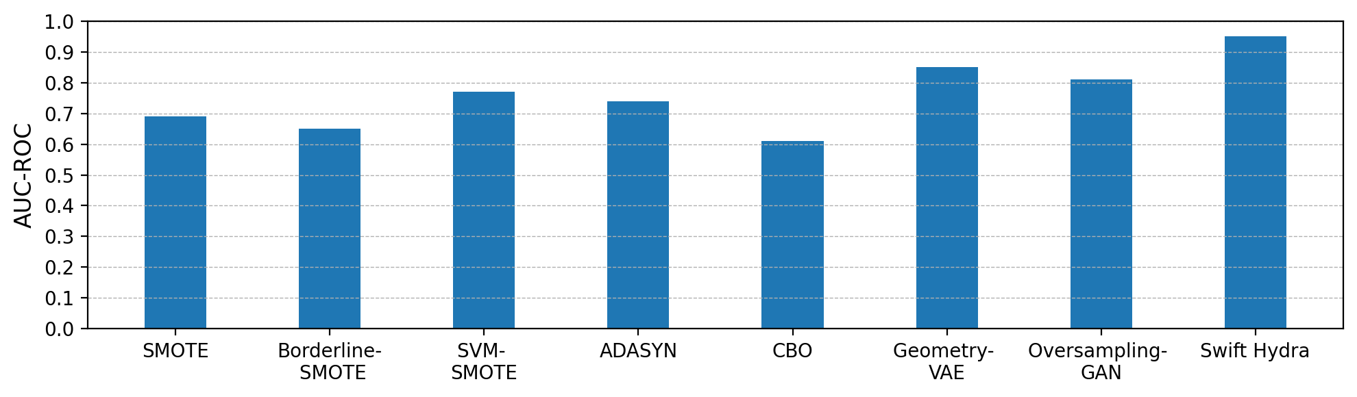
In addition to the previously discussed experiments, we also compare the performance of Swift Hydra against other oversampling methods using the AUC-ROC metric. As shown in Figure 3, our method is capable of generating the most diverse set of anomalous data points. The goal of this experiment is to assess how accurately Swift Hydra (MoME) performs given these diverse generated data points. Figure 5 presents a comparison of our method’s performance against various oversampling techniques included in the ADBench baselines. The results clearly demonstrate that Swift Hydra outperforms all other methods, achieving the highest AUC-ROC on the test set, with a 40/60% train/test ratio. This performance is primarily due to Swift Hydra’s ability to generate data points that extend beyond the boundaries of the training set.

Specifically, in the dataset illustrated in Figure 3, it is evident that the anomalous data points in the test set lie outside the boundaries of those in the training set. Traditional oversampling methods fail to generate data beyond these boundaries, which naturally results in a lower AUC-ROC on the test set. Deep learning-based oversampling methods, such as VAE-Geometry and Oversampling GAN, can produce more diverse data than traditional techniques. However, Oversampling GAN often encounters a model collapse issue, where it focuses on generating data points that deceive the detector very effectively, leading to an over-concentration of samples. On the other hand, VAE-Geometry relies on the geometric structure of the data for generation, but if the structure is too complex, it struggles to produce sufficiently diverse data points. As a result, both methods ultimately fall short of Swift Hydra in terms of AUC-ROC performance.

C.3 Toy Example: Generalization Ability and Decision Boundary on 2D Data

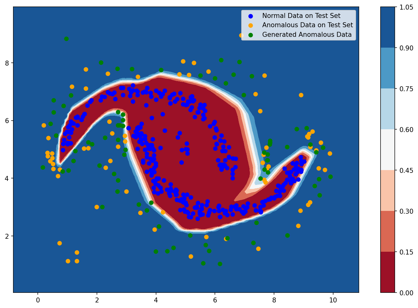
We conduct a toy example with 2D data to illustrate the generalization ability and decision boundary of the MoME module. First, we generate a dataset where the normal data follows a sine curve, while the anomalies are randomly distributed around the sine curve. Then, we use the Self-Reinforcing Module to generate additional anomalous data and visualize the boundary of the MoME in Figure 6.

From the visualization, we can observe that the red regions (indicating areas predicted by MoME as containing normal data) fully encapsulate the dark blue points (normal data). The blue regions (indicating areas predicted by MoME as containing anomalous data) completely cover the generated anomalous points (green) and the test set anomalies (orange). An interesting observation is that the green points (generated anomalies) cause the decision boundary to tightly enclose the dark blue points (normal data). This enhances MoME’s ability to accurately identify anomalous data in the test set, as these anomalies are positioned farther from the decision boundary. As expected, the model generalized well to the anomalies in the test set.

C.4 Ablation Study

C.4.1 Impact of Self-Reinforcing Module on Performance Across Deep Models

Methods	Transformer		Mamba		Swift Hydra(Transformer)		Swift Hydra(Mamba)
	AUCROC	TIF	AUCROC	TIF	AUCROC	TIF	AUCROC	TIF
Train/Test Ratio (40/60%)	0.78	5.18	0.80	3.54	0.90	7.96	0.93	4.01
Train/Test Ratio (30/70%)	0.75	6.07	0.77	3.62	0.88	8.79	0.91	4.79
Train/Test Ratio (20/80%)	0.72	7.10	0.73	4.11	0.86	9.91	0.90	5.22
Train/Test Ratio (10/90%)	0.69	8.22	0.71	4.63	0.82	10.36	0.87	5.84
TIF = Total Inference Time (Seconds)

Table 5: Comparison of Vanilla Transformer and Vanilla Mamba with Transformer and Mamba enhanced by the Self-Reinforcing Module in Swift Hydra, evaluated based on AUC-ROC and Total Inference Time (TIF).

Methods	Transformer (VAE-Geometry)		Mamba (VAE-Geometry)		Swift Hydra(Transformer)		Swift Hydra(Mamba)
	AUCROC	TIF	AUCROC	TIF	AUCROC	TIF	AUCROC	TIF
Train/Test Ratio (40/60%)	0.83	5.23	0.85	3.40	0.90	7.96	0.93	4.01
Train/Test Ratio (30/70%)	0.80	6.11	0.83	3.58	0.88	8.79	0.91	4.79
Train/Test Ratio (20/80%)	0.78	7.02	0.81	4.02	0.86	9.91	0.90	5.22
Train/Test Ratio (10/90%)	0.75	8.38	0.78	4.65	0.82	8.36	0.87	5.84
TIF = Total Inference Time (Seconds)

Table 6: AUC-ROC performance of various backbone models when applying oversampling techniques

We also compare the performance of Swift Hydra with various deep models (as backbone models) using two key metrics: AUC-ROC and Total Inference Time (for predicting the entire ADBench dataset) under two settings: with and without the use of an oversampling technique (i.e., VAE-Geometry). It is important to note that VAE-Geometry is chosen as the oversampling method for other backbone models due to its best performance among the oversampling baselines. As shown in Table 5 and Table 6, Swift Hydra outperforms other methods in terms of AUC-ROC while maintaining competitive total inference time.

AUC-ROC Evaluation. Regarding the accuracy in Table 5, standalone Mamba or Transformer models on ADBench exhibit significantly lower AUC-ROC compared to Swift Hydra (Mamba) and Swift Hydra (Transformer), which leverage the Self-Reinforcing Module. This is primarily because these models do not utilize any oversampling techniques (RL-guiled GenAI), which limits their data generalization capabilities. However, even when employing a powerful oversampling technique like VAE-Geometry (Table 6), the AUC-ROC of these models still falls short of that achieved by Swift Hydra. This is due to the fact that the datapoints generated by VAE-Geometry are not as diverse or of as high quality as those generated by Swift Hydra, as discussed in the previous experiment.

Total Inference Time Evaluation. In terms of total inference time, it is important to note that the Mamba model has a prediction complexity of O(1), while the Transformer has a prediction complexity of O(N). This makes Mamba substantially faster than both Transformer and Fully Connected networks. When Mamba is integrated into Swift Hydra with a Top $k$ Mixture of Experts ( $k=2$ ), one might expect the prediction time of Swift Hydra to be nearly double that of the regular Mamba model. However, the interesting outcome here is that we use only a two-layer depth for Mamba and overspecify the number of experts to 20. This allows us to capture the data complexity effectively, and since the model has just two layers, the additional time difference with $k=2$ is minimal compared to a larger Mamba model.

C.4.2 Impact of Probabilistic Cluster Assignment on MoME Performance

Method	Swift Hydra (MoME-Traditional Training Approach)		Swift Hydra (MoME-Our Training Approach)
	AUCROC	TIF	AUCROC	TIF
Train/Test Ratio (40/60%)	0.892	4.015	0.934	4.012
Train/Test Ratio (30/70%)	0.865	4.771	0.913	4.793
Train/Test Ratio (20/80%)	0.853	5.234	0.902	5.221
Train/Test Ratio (10/90%)	0.828	5.922	0.874	5.843

Table 7: Comparison of AUC-ROC and Total Inference Time (TIF) between Swift Hydra using the traditional MoME training approach and Swift Hydra with the proposed probabilistic training approach across different train/test ratios.

The results in Table 7 highlight a clear advantage of Swift Hydra with the proposed probabilistic training approach for MoME over the traditional MoME training approach. The primary reason for this improvement lies in addressing the “winner-take-all” problem that commonly affects the traditional training method.

In the traditional MoME approach, the gating network immediately starts assigning samples to experts based on their performance scores. During the early training steps, when the experts have not yet converged, their performance scores are arbitrary. This randomness can lead to one expert receiving disproportionately more samples than others, simply due to chance. As a result, this expert improves faster and continues to dominate sample assignments, creating a feedback loop where it becomes the sole contributor to predictions. This phenomenon, known as “winner-take-all,” reduces the diversity of the expert ensemble and significantly hinders the generalization ability of the model.

In contrast, Swift Hydra with the probabilistic training approach temporarily deactivates the gating network during the early training phase. Instead, it uses a probabilistic assignment mechanism (as described in Equation 6) to ensure that all experts receive equal opportunities to learn. Once the experts have sufficiently converged, the gating network is reactivated to assign samples based on their performance. This method prevents any single expert from monopolizing the training process early on and ensures a more balanced and effective ensemble.

The results in the table demonstrate that this improved training strategy consistently achieves higher AUC-ROC scores across all train/test ratios compared to the traditional approach, without incurring additional Total Inference Time (TIF). This validates the effectiveness of addressing the ”winner-take-all” problem to enhance both the generalization and overall performance of the model.

C.4.3 KL Divergence and Reconstruction Loss Trade-off in Conditional Variational Auto Encoder

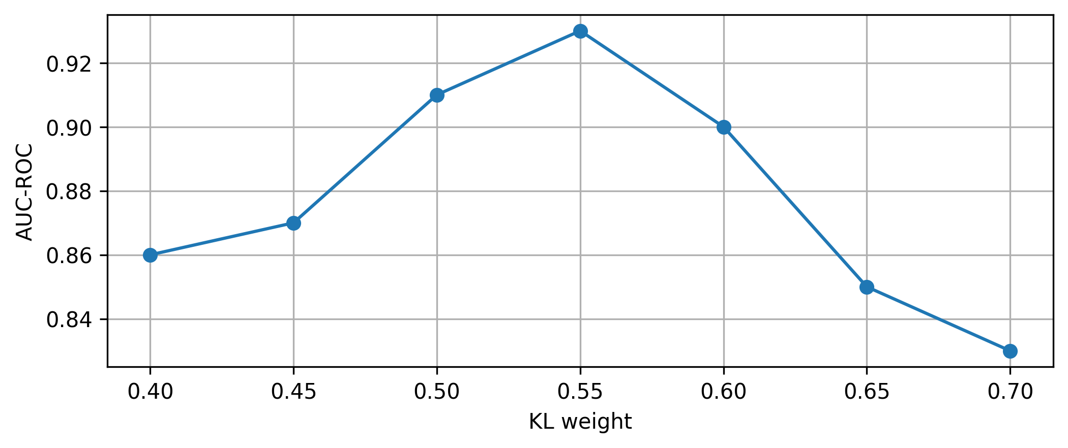
In this section, we provide insights into how the weight impacts the C-VAE during data generation. Specifically, when optimizing the ELBO loss of C-VAE, we need to consider two components: the Reconstruction Loss and the KL Loss. If more weight is placed on the Reconstruction Loss, the C-VAE will generate data more cautiously, closely adhering to the target class. However, this caution results in less diverse samples. Conversely, if the weight is placed more on the KL Loss, the C-VAE generates more diverse data, but it may also produce samples that overlap with other classes.

To identify the optimal weight for the KL Loss, we experimented with various values of $p$ ranging from 0.4 to 0.7. If the weight for the KL Loss is $p$ , the weight for the Reconstruction Loss will be $1-p$ . As shown in Figure 7, the optimal weight for the KL Loss is found to be 0.55. In the range of 0.4 to 0.5, the C-VAE generates overly cautious samples, resulting in a lack of diversity. Consequently, the 200 episodes of RL training are insufficient to cover the entire set of anomalous data in the test set. On the other hand, in the range of 0.6 to 0.7, the model focuses too much on optimizing the KL Loss, leading to the generation of highly diverse anomalous samples. However, these samples tend to overlap significantly with normal samples, causing Swift Hydra’s performance to decline after 200 episodes.

C.5 RL-Agent Assistance Frequency Experiment

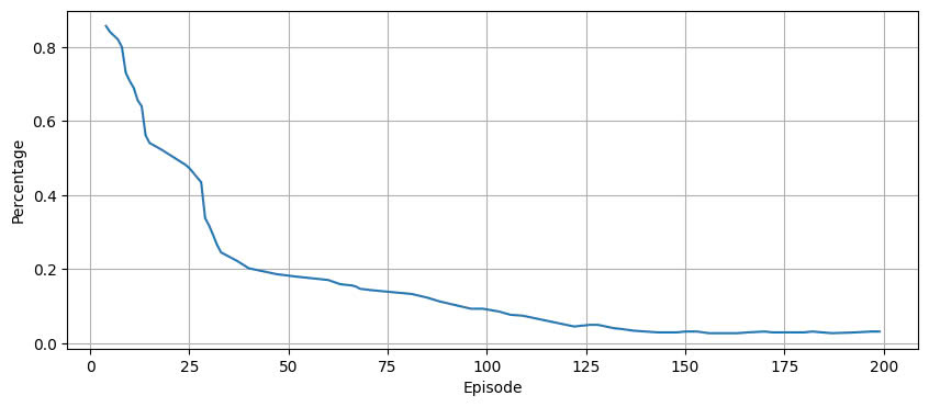
In this section, we illustrate the average percentage of invalid actions taken by the agent in each episode (averaged over 57 datasets from ADBench). From Figure 8, it is evident that in the initial stages, the RL-Agent generates a high number of invalid actions, frequently requiring assistance from the One-Step to Feasible Action algorithm described in Section 3.1.2. However, since every time the RL-Agent takes an invalid action, it learns in a supervised manner using the feasible action provided by the One-Step to Feasible Action algorithm, a significant reduction in invalid actions is observed after about 25 to 50 episodes.

As a result, the training time becomes considerably faster since fewer Gradient Descent steps are needed (as Gradient Descent is primarily performed to optimize the reward function whenever an invalid action is taken). From episode 150 onward, the RL-Agent rarely makes invalid actions, and its actions become highly effective (as reflected in the AUC-ROC in previous experiment), indicating that the RL-Agent has successfully generalized.

C.6 Datasets In ADBench

ADBench features a comprehensive collection of 57 datasets designed for anomaly detection research, as detailed in the table. Among these, 47 datasets are well-established and widely used across various real-world domains, such as healthcare (e.g., disease diagnosis), audio and language processing (e.g., speech recognition), image analysis (e.g., object identification), and finance (e.g., fraud detection). Additionally, ADBench introduces 10 more complex datasets from computer vision (CV) and natural language processing (NLP) domains, enriched with larger sample sizes and higher-dimensional features. These datasets utilize pretrained models to extract embeddings, enabling the representation of more complex patterns. All datasets are provided in a user-friendly format as compressed NumPy array files (‘.npz‘), with detailed instructions and processing codes available for seamless application

Table 8: Summary of Datasets used in ADBench Benchmark. The table outlines key characteristics of 57 anomaly detection datasets, including the number of samples, features, anomalies, and their respective categories, spanning diverse domains such as image analysis, healthcare, finance, and natural language processing.

Number	Data	# Samples	# Features	# Anomaly	% Anomaly	Category
1	ALOI	49534	27	1508	3.04	Image
2	annthyroid	7200	6	534	7.42	Healthcare
3	backdoor	95329	196	2329	2.44	Network
4	breastw	683	9	239	34.99	Healthcare
5	campaign	41188	62	4640	11.27	Finance
6	cardio	1831	21	176	9.61	Healthcare
7	Cardiotocography	2114	21	466	22.04	Healthcare
8	celeba	202599	39	4547	2.24	Image
9	census	299285	500	18568	6.20	Sociology
10	cover	286048	10	2747	0.96	Botany
11	donors	619326	10	36710	5.93	Sociology
12	fault	1941	27	673	34.67	Physical
13	fraud	284807	29	492	0.17	Finance
14	glass	214	7	9	4.21	Forensic
15	Hepatitis	80	19	13	16.25	Healthcare
16	http	567498	3	2211	0.39	Web
17	InternetAds	1966	1555	368	18.72	Image
18	Ionosphere	351	32	126	35.90	Oryctognosy
19	landsat	6435	36	1333	20.71	Astronautics
20	letter	1600	32	100	6.25	Image
21	Lymphography	148	18	6	4.05	Healthcare
22	magic.gamma	19020	10	6688	35.16	Physical
23	mammography	11183	6	260	2.32	Healthcare
24	mnist	7603	100	700	9.21	Image
25	musk	3062	166	97	3.17	Chemistry
26	optdigits	5216	64	150	2.88	Image
27	PageBlocks	5393	10	510	9.46	Document
28	pendigits	6870	16	156	2.27	Image
29	Pima	768	8	268	34.90	Healthcare
30	satellite	6435	36	2036	31.64	Astronautics
31	satimage-2	5803	36	71	1.22	Astronautics
32	shuttle	49097	9	3511	7.15	Astronautics
33	skin	245057	3	50859	20.75	Image
34	smtp	95156	3	30	0.03	Web
35	SpamBase	4207	57	1679	39.91	Document
36	speech	3686	400	61	1.65	Linguistics
37	Stamps	340	9	31	9.12	Document
38	thyroid	3772	6	93	2.47	Healthcare
39	vertebral	240	6	30	12.50	Biology
40	vowels	1456	12	50	3.43	Linguistics
41	Waveform	3443	21	100	2.90	Physics
42	WBC	223	9	10	4.48	Healthcare
43	WDBC	367	30	10	2.72	Healthcare
44	Wilt	4819	5	257	5.33	Botany
45	wine	129	13	10	7.75	Chemistry
46	WPBC	198	33	47	23.74	Healthcare
47	yeast	1484	8	507	34.16	Biology
48	CIFAR10	5263	512	263	5.00	Image
49	FashionMNIST	6315	512	315	5.00	Image
50	MNIST-C	10000	512	500	5.00	Image
51	MVTec-AD	5354	512	1258	23.50	Image
52	SVHN	5208	512	260	5.00	Image
53	Agnews	10000	768	500	5.00	NLP
54	Amazon	10000	768	500	5.00	NLP
55	Imdb	10000	768	500	5.00	NLP
56	Yelp	10000	768	500	5.00	NLP
57	20newsgroups	11905	768	591	4.96	NLP

C.7 Swift Hydra: Class-Wise Precision, Recall, and F1-Score on ADBENCH

This final section provides a comprehensive comparison of various state-of-the-art anomaly detection methods, including DTE, Rejex, and ADGym, against Swift Hydra across 57 datasets from ADBench. The evaluation criteria include Precision, Recall, F1 score, support for each class, and AUC-ROC. It is important to note that we did not set a unique threshold for each individual dataset; instead, we applied a common threshold across all 57 datasets in ADBench. As a result, the Precision might not be very high. However, the focus should also be on the Recall and AUC-ROC, as these metrics more accurately reflect the model’s ability to detect anomalous data if the correct threshold is chosen. This approach gives a clearer picture of how well Swift Hydra can identify anomalies in various datasets.

	DTE			Rejex			ADGym			Swift Hydra
ALOI	P	R	F1	P	R	F1	P	R	F1	P	R	F1	support
-1	0.97	0.97	0.97	0.97	0.95	0.96	0.92	0.38	0.54	0.99	0.44	0.61	28821
1	0.03	0.03	0.03	0.04	0.07	0.05	0.00	0.75	0.05	0.04	0.81	0.08	900
accuracy	0.94			0.92			0.39			0.45			29721
macro avg	0.50	0.50	0.50	0.50	0.51	0.50	0.46	0.57	0.30	0.52	0.63	0.35	29721
weighted avg	0.94	0.94	0.94	0.94	0.92	0.93	0.89	0.39	0.53	0.96	0.45	0.60	29721
AUC-ROC	0.535			0.53			0.66			0.70
annthyroid	P	R	F1	P	R	F1	P	R	F1	P	R	F1	support
-1	0.94	0.95	0.95	0.98	0.94	0.96	0.95	0.88	0.92	1.00	0.95	0.97	4001
1	0.32	0.29	0.31	0.52	0.77	0.62	0.56	0.92	0.71	0.60	0.98	0.75	319
accuracy	0.90			0.93			0.89			0.95			4320
macro avg	0.63	0.62	0.63	0.75	0.86	0.79	0.75	0.90	0.82	0.80	0.97	0.86	4320
weighted avg	0.90	0.90	0.90	0.95	0.93	0.94	0.92	0.89	0.91	0.97	0.95	0.96	4320
AUC-ROC	0.81			0.96			0.93			0.98
backdoor	P	R	F1	P	R	F1	P	R	F1	P	R	F1	support
-1	0.98	0.98	0.98	0.99	0.99	0.99	0.94	0.95	0.96	1.00	0.99	0.99	55790
1	0.01	0.01	0.01	0.68	0.47	0.56	0.55	0.89	0.67	0.61	0.92	0.74	1408
accuracy	0.95			0.98			0.95			0.98			57198
macro avg	0.49	0.49	0.49	0.83	0.73	0.77	0.75	0.92	0.82	0.81	0.95	0.86	57198
weighted avg	0.95	0.95	0.95	0.98	0.98	0.98	0.93	0.95	0.95	0.99	0.98	0.99	57198
AUC-ROC	0.76			0.90			0.94			0.98
breastw	P	R	F1	P	R	F1	P	R	F1	P	R	F1	support
-1	0.99	0.94	0.97	1.00	0.69	0.82	0.95	0.93	0.94	0.99	0.97	0.98	264
1	0.91	0.99	0.94	0.64	1.00	0.78	0.88	0.92	0.91	0.94	0.98	0.96	146
accuracy	0.96			0.80			0.93			0.97			410
macro avg	0.95	0.97	0.96	0.82	0.85	0.80	0.92	0.92	0.92	0.97	0.97	0.97	410
weighted avg	0.96	0.96	0.96	0.87	0.80	0.80	0.93	0.93	0.93	0.97	0.97	0.97	410
AUC-ROC	0.99			0.93			0.94			0.99
campaign	P	R	F1	P	R	F1	P	R	F1	P	R	F1	support
-1	0.91	0.91	0.91	0.89	0.99	0.94	0.92	0.79	0.85	0.98	0.82	0.89	21920
1	0.32	0.32	0.32	0.27	0.04	0.08	0.33	0.79	0.47	0.38	0.83	0.52	2793
accuracy	0.84			0.88			0.79			0.83			24713
macro avg	0.62	0.62	0.62	0.58	0.51	0.51	0.63	0.79	0.66	0.68	0.83	0.71	24713
weighted avg	0.85	0.84	0.85	0.82	0.88	0.84	0.86	0.79	0.81	0.91	0.83	0.85	24713
AUC-ROC	0.73			0.77			0.84			0.90
cardio	P	R	F1	P	R	F1	P	R	F1	P	R	F1	support
-1	0.94	0.92	0.93	0.94	0.82	0.87	0.95	0.88	0.93	0.99	0.94	0.97	990
1	0.42	0.50	0.45	0.23	0.51	0.32	0.57	0.89	0.72	0.64	0.95	0.76	109
accuracy	0.88			0.79			0.88			0.94			1099
macro avg	0.68	0.71	0.69	0.59	0.66	0.60	0.76	0.88	0.83	0.82	0.94	0.86	1099
weighted avg	0.89	0.88	0.89	0.87	0.79	0.82	0.91	0.88	0.91	0.96	0.94	0.95	1099
AUC-ROC	0.92			0.74			0.95			0.98
Cardiotocography	P	R	F1	P	R	F1	P	R	F1	P	R	F1	support
-1	0.82	0.83	0.82	0.80	0.75	0.78	0.92	0.83	0.90	0.98	0.90	0.93	991
1	0.37	0.36	0.36	0.27	0.33	0.30	0.68	0.87	0.74	0.71	0.92	0.80	278
accuracy	0.72			0.66			0.84			0.90			1269
macro avg	0.59	0.59	0.59	0.54	0.54	0.54	0.80	0.85	0.82	0.84	0.91	0.87	1269
weighted avg	0.72	0.72	0.72	0.68	0.66	0.67	0.87	0.84	0.87	0.92	0.90	0.91	1269
AUC-ROC	0.73			0.53			0.91			0.95
celeba	P	R	F1	P	R	F1	P	R	F1	P	R	F1	support
-1	0.98	0.98	0.98	0.98	1.00	0.99	0.96	0.83	0.88	1.00	0.89	0.94	118850
1	0.09	0.09	0.09	0.03	0.00	0.00	0.11	0.85	0.21	0.15	0.91	0.26	2710
accuracy	0.96			0.98			0.83			0.89			121560
macro avg	0.53	0.53	0.53	0.50	0.50	0.50	0.53	0.84	0.55	0.58	0.90	0.60	121560
weighted avg	0.96	0.96	0.96	0.96	0.98	0.97	0.94	0.83	0.86	0.98	0.89	0.92	121560
AUC-ROC	0.72			0.79			0.88			0.95
census	P	R	F1	P	R	F1	P	R	F1	P	R	F1	support
-1	0.94	0.94	0.94	0.94	0.88	0.91	0.92	0.72	0.84	0.99	0.79	0.88	168432
1	0.04	0.04	0.04	0.06	0.12	0.08	0.15	0.77	0.31	0.21	0.84	0.34	11139
accuracy	0.88			0.84			0.73			0.79			179571
macro avg	0.49	0.49	0.49	0.50	0.50	0.50	0.54	0.75	0.58	0.60	0.82	0.61	179571
weighted avg	0.88	0.88	0.88	0.88	0.84	0.86	0.87	0.73	0.81	0.94	0.79	0.84	179571
AUC-ROC	0.59			0.65			0.79			0.85
cover	P	R	F1	P	R	F1	P	R	F1	P	R	F1	support
-1	0.99	0.99	0.99	0.99	0.99	0.99	0.95	0.96	0.94	1.00	0.99	1.00	169976
1	0.09	0.09	0.09	0.06	0.05	0.06	0.50	0.95	0.65	0.54	1.00	0.70	1653
accuracy	0.98			0.98			0.96			0.99			171629
macro avg	0.54	0.54	0.54	0.53	0.52	0.52	0.73	0.96	0.80	0.77	0.99	0.85	171629
weighted avg	0.98	0.98	0.98	0.98	0.98	0.98	0.95	0.96	0.94	1.00	0.99	0.99	171629
AUC-ROC	0.90			0.74			0.97			1.00
donors	P	R	F1	P	R	F1	P	R	F1	P	R	F1	support
-1	0.94	0.94	0.94	0.94	0.99	0.96	0.93	0.95	0.94	1.00	1.00	1.00	349483
1	0.10	0.10	0.10	0.14	0.03	0.05	0.95	0.95	0.95	1.00	1.00	1.00	22113
accuracy	0.89			0.93			0.95			1.00			371596
macro avg	0.52	0.52	0.52	0.54	0.51	0.51	0.94	0.95	0.94	1.00	1.00	1.00	371596
weighted avg	0.89	0.89	0.89	0.89	0.93	0.91	0.93	0.95	0.94	1.00	1.00	1.00	371596
AUC-ROC	0.76			0.74			0.95			1.00
fault	P	R	F1	P	R	F1	P	R	F1	P	R	F1	support
-1	0.69	0.66	0.68	0.68	0.89	0.77	0.78	0.62	0.69	0.81	0.65	0.72	751
1	0.43	0.45	0.44	0.53	0.23	0.32	0.49	0.68	0.57	0.54	0.73	0.62	414
accuracy	0.59			0.65			0.64			0.68			1165
macro avg	0.56	0.56	0.56	0.60	0.56	0.54	0.63	0.65	0.63	0.67	0.69	0.67	1165
weighted avg	0.60	0.59	0.59	0.62	0.65	0.61	0.67	0.64	0.65	0.71	0.68	0.69	1165
AUC-ROC	0.54			0.58			0.68			0.74
fraud	P	R	F1	P	R	F1	P	R	F1	P	R	F1	support
-1	1.00	1.00	1.00	1.00	0.99	1.00	0.96	0.86	0.91	1.00	0.92	0.96	170593
1	0.30	0.28	0.29	0.13	0.81	0.22	0.00	0.85	0.00	0.02	0.92	0.04	292
accuracy	1.00			0.99			0.86			0.92			170885
macro avg	0.65	0.64	0.65	0.56	0.90	0.61	0.48	0.85	0.45	0.51	0.92	0.50	170885
weighted avg	1.00	1.00	1.00	1.00	0.99	0.99	0.96	0.86	0.91	1.00	0.92	0.96	170885
AUC-ROC	0.95			0.95			0.92			0.96
glass	P	R	F1	P	R	F1	P	R	F1	P	R	F1	support
-1	0.95	0.98	0.96	0.00	0.00	0.00	0.93	0.75	0.83	0.96	0.81	0.88	123
1	0.00	0.00	0.00	0.05	1.00	0.09	0.04	0.27	0.09	0.08	0.33	0.13	6
accuracy	0.93			0.05			0.73			0.79			129
macro avg	0.48	0.49	0.48	0.02	0.50	0.04	0.48	0.51	0.46	0.52	0.57	0.51	129
weighted avg	0.91	0.93	0.92	0.00	0.05	0.00	0.89	0.73	0.80	0.92	0.79	0.85	129
AUC-ROC	0.76			0.75			0.78			0.84
Hepatitis	P	R	F1	P	R	F1	P	R	F1	P	R	F1	support
-1	0.85	0.83	0.84	0.00	0.00	0.00	0.90	0.62	0.75	0.97	0.67	0.79	42
1	0.00	0.00	0.00	0.13	1.00	0.22	0.22	0.79	0.33	0.26	0.83	0.40	6
accuracy	0.73			0.13			0.64			0.69			0.69
macro avg	0.43	0.42	0.42	0.06	0.50	0.11	0.56	0.71	0.54	0.61	0.75	0.59	48
weighted avg	0.75	0.73	0.74	0.02	0.13	0.03	0.81	0.64	0.70	0.88	0.69	0.74	48
AUC-ROC	0.72			0.42			0.74			0.80
http	P	R	F1	P	R	F1	P	R	F1	P	R	F1	support
-1	1.00	1.00	1.00	1.00	0.94	0.97	0.95	0.96	0.94	1.00	1.00	1.00	339161
1	0.23	0.02	0.03	0.06	1.00	0.12	0.72	0.95	0.79	0.76	1.00	0.86	1338
accuracy	1.00			0.94			0.96			1.00			340499
macro avg	0.61	0.51	0.51	0.53	0.97	0.54	0.84	0.96	0.87	0.88	1.00	0.93	340499
weighted avg	0.99	1.00	0.99	1.00	0.94	0.97	0.95	0.96	0.94	1.00	1.00	1.00	340499
AUC-ROC	1.00			1.00			0.94			1.00
InternetAds	P	R	F1	P	R	F1	P	R	F1	P	R	F1	support
-1	0.88	0.88	0.88	0.89	0.44	0.59	0.93	0.63	0.74	0.98	0.68	0.81	965
1	0.45	0.46	0.46	0.23	0.75	0.35	0.37	0.88	0.53	0.40	0.94	0.56	215
accuracy	0.80			0.50			0.67			0.73			1180
macro avg	0.67	0.67	0.67	0.56	0.60	0.47	0.65	0.75	0.63	0.69	0.81	0.68	1180
weighted avg	0.80	0.80	0.80	0.77	0.50	0.55	0.83	0.67	0.70	0.88	0.73	0.76	1180
AUC-ROC	0.68			0.67			0.88			0.92
Ionosphere	P	R	F1	P	R	F1	P	R	F1	P	R	F1	support
-1	0.82	0.76	0.79	0.00	0.00	0.00	0.86	0.85	0.84	0.90	0.90	0.90	135
1	0.62	0.70	0.65	0.36	1.00	0.53	0.76	0.78	0.76	0.83	0.82	0.82	76
accuracy	0.74			0.36			0.82			0.87			211
macro avg	0.72	0.73	0.72	0.18	0.50	0.27	0.81	0.81	0.80	0.86	0.86	0.86	211
weighted avg	0.74	0.74	0.74	0.13	0.36	0.19	0.82	0.82	0.81	0.87	0.87	0.87	211
AUC-ROC	0.86			0.96			0.85			0.91
landsat	P	R	F1	P	R	F1	P	R	F1	P	R	F1	support
-1	0.81	0.79	0.80	0.80	0.94	0.86	0.92	0.80	0.86	0.97	0.86	0.91	3068
1	0.24	0.26	0.25	0.23	0.06	0.10	0.56	0.83	0.68	0.62	0.89	0.73	793
accuracy	0.68			0.76			0.80			0.87			3861
macro avg	0.52	0.52	0.52	0.51	0.50	0.48	0.74	0.81	0.77	0.79	0.87	0.82	3861
weighted avg	0.69	0.68	0.68	0.68	0.76	0.71	0.85	0.80	0.82	0.90	0.87	0.87	3861
AUC-ROC	0.50			0.53			0.91			0.94
letter	P	R	F1	P	R	F1	P	R	F1	P	R	F1	support
-1	0.94	0.94	0.94	0.98	0.65	0.78	0.94	0.76	0.83	0.98	0.82	0.89	900
1	0.09	0.10	0.10	0.14	0.83	0.24	0.16	0.63	0.27	0.20	0.68	0.31	60
accuracy	0.88			0.66			0.75			0.81			960
macro avg	0.52	0.52	0.52	0.56	0.74	0.51	0.55	0.69	0.55	0.59	0.75	0.60	960
weighted avg	0.89	0.88	0.89	0.93	0.66	0.75	0.89	0.75	0.80	0.93	0.81	0.85	960
AUC-ROC	0.57			0.85			0.77			0.80
Lymphography	P	R	F1	P	R	F1	P	R	F1	P	R	F1	support
-1	1.00	0.95	0.98	0.00	0.00	0.00	0.90	0.94	0.92	0.95	0.99	0.97	84
1	0.56	1.00	0.71	0.06	1.00	0.11	0.47	0.17	0.24	0.50	0.20	0.29	5
accuracy	0.96			0.06			0.90			0.94			89
macro avg	0.78	0.98	0.85	0.03	0.50	0.05	0.68	0.56	0.58	0.73	0.59	0.63	89
weighted avg	0.98	0.96	0.96	0.00	0.06	0.01	0.88	0.90	0.89	0.93	0.94	0.93	89
AUC-ROC	0.99			0.99			0.64			0.69
magic.gamma	P	R	F1	P	R	F1	P	R	F1	P	R	F1	support
-1	0.75	0.75	0.75	0.72	0.95	0.82	0.87	0.69	0.76	0.93	0.74	0.82	7422
1	0.54	0.55	0.54	0.75	0.31	0.44	0.60	0.86	0.71	0.65	0.90	0.75	3990
accuracy	0.68			0.72			0.75			0.79			11412
macro avg	0.65	0.65	0.65	0.74	0.63	0.63	0.73	0.77	0.74	0.79	0.82	0.79	11412
weighted avg	0.68	0.68	0.68	0.73	0.72	0.69	0.77	0.75	0.75	0.83	0.79	0.80	11412
AUC-ROC	0.73			0.76			0.88			0.92
mammography	P	R	F1	P	R	F1	P	R	F1	P	R	F1	support
-1	0.98	0.98	0.98	0.99	0.83	0.90	0.93	0.80	0.90	1.00	0.87	0.93	6558
1	0.25	0.26	0.25	0.08	0.62	0.14	0.06	0.83	0.17	0.13	0.88	0.23	152
accuracy	0.97			0.82			0.80			0.87			6710
macro avg	0.62	0.62	0.62	0.53	0.72	0.52	0.50	0.82	0.53	0.56	0.87	0.58	6710
weighted avg	0.97	0.97	0.97	0.97	0.82	0.88	0.91	0.80	0.88	0.98	0.87	0.91	6710
AUC-ROC	0.86			0.84			0.86			0.91
mnist	P	R	F1	P	R	F1	P	R	F1	P	R	F1	support
-1	0.93	0.93	0.93	0.94	0.97	0.95	0.94	0.89	0.91	1.00	0.94	0.97	4172
1	0.29	0.30	0.29	0.46	0.28	0.35	0.57	0.91	0.70	0.60	0.97	0.74	390
accuracy	0.88			0.91			0.90			0.94			4562
macro avg	0.61	0.61	0.61	0.70	0.62	0.65	0.76	0.90	0.80	0.80	0.95	0.85	4562
weighted avg	0.88	0.88	0.88	0.89	0.91	0.90	0.91	0.90	0.89	0.96	0.94	0.95	4562
AUC-ROC	0.77			0.79			0.92			0.98
musk	P	R	F1	P	R	F1	P	R	F1	P	R	F1	support
-1	1.00	1.00	1.00	0.98	1.00	0.99	0.96	0.93	0.95	1.00	1.00	1.00	1777
1	0.95	1.00	0.98	0.72	0.34	0.47	0.95	0.94	0.96	1.00	1.00	1.00	61
accuracy	1.00			0.97			0.93			1.00			1838
macro avg	0.98	1.00	0.99	0.85	0.67	0.73	0.95	0.94	0.95	1.00	1.00	1.00	1838
weighted avg	1.00	1.00	1.00	0.97	0.97	0.97	0.96	0.93	0.95	1.00	1.00	1.00	1838
AUC-ROC	1.00			0.96			0.94			1.00
optdigits	P	R	F1	P	R	F1	P	R	F1	P	R	F1	support
-1	0.97	0.96	0.97	0.97	0.88	0.92	0.94	0.91	0.92	1.00	0.97	0.98	3044
1	0.01	0.01	0.01	0.00	0.01	0.00	0.38	0.97	0.59	0.45	1.00	0.62	86
accuracy	0.94			0.86			0.91			0.97			3130
macro avg	0.49	0.49	0.49	0.49	0.45	0.46	0.66	0.94	0.75	0.72	0.98	0.80	3130
weighted avg	0.95	0.94	0.94	0.94	0.86	0.90	0.93	0.91	0.91	0.99	0.97	0.97	3130
AUC-ROC	0.71			0.36			0.97			1.00
PageBlocks	P	R	F1	P	R	F1	P	R	F1	P	R	F1	support
-1	0.94	0.94	0.94	0.97	0.95	0.96	0.94	0.86	0.89	1.00	0.92	0.95	2916
1	0.43	0.45	0.44	0.59	0.69	0.64	0.49	0.90	0.66	0.56	0.96	0.71	320
accuracy	0.89			0.92			0.86			0.92			3236
macro avg	0.69	0.69	0.69	0.78	0.82	0.80	0.72	0.88	0.78	0.78	0.94	0.83	3236
weighted avg	0.89	0.89	0.89	0.93	0.92	0.93	0.90	0.86	0.87	0.95	0.92	0.93	3236
AUC-ROC	0.92			0.95			0.92			0.98
pendigits	P	R	F1	P	R	F1	P	R	F1	P	R	F1	support
-1	0.98	0.98	0.98	0.99	0.82	0.89	0.95	0.93	0.94	1.00	0.98	0.99	4032
1	0.26	0.26	0.26	0.07	0.59	0.12	0.50	0.94	0.68	0.56	0.99	0.72	90
accuracy	0.97			0.81			0.93			0.98			4122
macro avg	0.62	0.62	0.62	0.53	0.70	0.51	0.72	0.93	0.81	0.78	0.99	0.85	4122
weighted avg	0.97	0.97	0.97	0.97	0.81	0.88	0.94	0.93	0.94	0.99	0.98	0.99	4122
AUC-ROC	0.93			0.83			0.95			1.00
Pima	P	R	F1	P	R	F1	P	R	F1	P	R	F1	support
-1	0.73	0.66	0.69	0.00	0.00	0.00	0.74	0.59	0.66	0.78	0.64	0.70	294
1	0.48	0.56	0.52	0.36	1.00	0.53	0.48	0.60	0.54	0.52	0.67	0.58	167
accuracy	0.62			0.36			0.60			0.65			461
macro avg	0.60	0.61	0.60	0.18	0.50	0.27	0.61	0.60	0.60	0.65	0.66	0.64	461
weighted avg	0.64	0.62	0.63	0.13	0.36	0.19	0.65	0.60	0.62	0.68	0.65	0.66	461
AUC-ROC	0.66			0.57			0.66			0.70
satellite	P	R	F1	P	R	F1	P	R	F1	P	R	F1	support
-1	0.81	0.79	0.80	0.70	0.98	0.82	0.91	0.84	0.86	0.96	0.88	0.92	2626
1	0.58	0.62	0.60	0.75	0.11	0.20	0.74	0.89	0.80	0.79	0.92	0.85	1235
accuracy	0.74			0.70			0.86			0.89			3861
macro avg	0.70	0.70	0.70	0.72	0.55	0.51	0.82	0.87	0.83	0.87	0.90	0.88	3861
weighted avg	0.74	0.74	0.74	0.72	0.70	0.62	0.85	0.86	0.84	0.90	0.89	0.90	3861
AUC-ROC	0.70			0.73			0.89			0.96
satimage-2	P	R	F1	P	R	F1	P	R	F1	P	R	F1	support
-1	1.00	1.00	1.00	1.00	0.93	0.96	0.97	0.93	0.96	1.00	0.98	0.99	3440
1	0.80	0.83	0.81	0.13	0.86	0.22	0.30	0.86	0.46	0.36	0.91	0.52	42
accuracy	1.00			0.93			0.93			0.98			3482
macro avg	0.90	0.92	0.91	0.56	0.89	0.59	0.63	0.89	0.71	0.68	0.94	0.75	3482
weighted avg	1.00	1.00	1.00	0.99	0.93	0.95	0.96	0.93	0.95	0.99	0.98	0.98	3482
AUC-ROC	0.99			0.97			0.94			0.99
shuttle	P	R	F1	P	R	F1	P	R	F1	P	R	F1	support
-1	0.99	1.00	1.00	0.94	1.00	0.96	0.97	0.96	0.94	1.00	1.00	1.00	27388
1	0.95	0.92	0.93	0.55	0.09	0.15	0.91	0.93	0.92	0.95	1.00	0.98	2071
accuracy	0.99			0.93			0.96			1.00			29459
macro avg	0.97	0.96	0.96	0.74	0.54	0.56	0.94	0.94	0.93	0.98	1.00	0.99	29459
weighted avg	0.99	0.99	0.99	0.91	0.93	0.91	0.96	0.96	0.94	1.00	1.00	1.00	29459
AUC-ROC	1.00			0.99			0.95			1.00
skin	P	R	F1	P	R	F1	P	R	F1	P	R	F1	support
-1	0.76	0.76	0.76	0.79	0.79	0.79	0.94	0.94	0.94	1.00	1.00	1.00	116448
1	0.09	0.09	0.09	0.19	0.18	0.18	0.95	0.94	0.96	1.00	1.00	1.00	30587
accuracy	0.62			0.66			0.94			1.00			147035
macro avg	0.42	0.43	0.42	0.49	0.49	0.49	0.95	0.94	0.95	1.00	1.00	1.00	147035
weighted avg	0.62	0.62	0.62	0.66	0.66	0.66	0.94	0.94	0.94	1.00	1.00	1.00	147035
AUC-ROC	0.68			0.74			0.94			1.00
smtp	P	R	F1	P	R	F1	P	R	F1	P	R	F1	support
-1	1.00	1.00	1.00	1.00	0.68	0.81	0.95	0.85	0.91	1.00	0.90	0.95	57075
1	0.00	0.00	0.00	0.00	1.00	0.00	0.00	0.81	0.00	0.00	0.84	0.01	19
accuracy	1.00			0.68			0.85			0.90			57094
macro avg	0.50	0.50	0.50	0.50	0.84	0.41	0.48	0.83	0.45	0.50	0.87	0.48	57094
weighted avg	1.00	1.00	1.00	1.00	0.68	0.81	0.95	0.85	0.91	1.00	0.90	0.95	57094
AUC-ROC	0.92			0.95			0.81			0.85
SpamBase	P	R	F1	P	R	F1	P	R	F1	P	R	F1	support
-1	0.65	0.67	0.66	0.58	0.64	0.61	0.92	0.81	0.86	0.96	0.86	0.91	1513
1	0.49	0.47	0.48	0.37	0.32	0.34	0.77	0.89	0.84	0.82	0.95	0.88	1012
accuracy	0.59			0.51			0.84			0.89			2525
macro avg	0.57	0.57	0.57	0.48	0.48	0.48	0.84	0.85	0.85	0.89	0.90	0.89	2525
weighted avg	0.59	0.59	0.59	0.50	0.51	0.50	0.86	0.84	0.85	0.90	0.89	0.89	2525
AUC-ROC	0.61			0.51			0.92			0.95
speech	P	R	F1	P	R	F1	P	R	F1	P	R	F1	support
-1	0.98	0.99	0.99	0.99	0.13	0.23	0.93	0.49	0.67	1.00	0.53	0.70	2177
1	0.00	0.00	0.00	0.02	0.91	0.03	0.00	0.83	0.01	0.03	0.89	0.06	35
accuracy	0.97			0.15			0.49			0.54			2212
macro avg	0.49	0.49	0.49	0.50	0.52	0.13	0.47	0.66	0.34	0.51	0.71	0.38	2212
weighted avg	0.97	0.97	0.97	0.97	0.15	0.23	0.92	0.49	0.65	0.98	0.54	0.69	2212
AUC-ROC	0.47			0.47			0.67			0.73
Stamps	P	R	F1	P	R	F1	P	R	F1	P	R	F1	support
-1	0.97	0.90	0.93	0.00	0.00	0.00	0.96	0.79	0.87	1.00	0.86	0.92	185
1	0.41	0.68	0.51	0.09	1.00	0.17	0.39	0.94	0.54	0.42	1.00	0.59	19
accuracy	0.88			0.09			0.81			0.87			204
macro avg	0.69	0.79	0.72	0.05	0.50	0.09	0.67	0.87	0.70	0.71	0.93	0.76	204
weighted avg	0.91	0.88	0.89	0.01	0.09	0.02	0.91	0.81	0.84	0.95	0.87	0.89	204
AUC-ROC	0.89			0.74			0.93			0.96
thyroid	P	R	F1	P	R	F1	P	R	F1	P	R	F1	support
-1	0.99	0.99	0.99	1.00	0.88	0.94	0.96	0.93	0.92	1.00	0.97	0.99	2207
1	0.63	0.65	0.64	0.18	0.98	0.30	0.43	0.97	0.60	0.49	1.00	0.66	57
accuracy	0.98			0.88			0.93			0.97			2264
macro avg	0.81	0.82	0.81	0.59	0.93	0.62	0.69	0.95	0.76	0.75	0.99	0.82	2264
weighted avg	0.98	0.98	0.98	0.98	0.88	0.92	0.94	0.93	0.91	0.99	0.97	0.98	2264
AUC-ROC	0.98			0.99			0.94			1.00
vertebral	P	R	F1	P	R	F1	P	R	F1	P	R	F1	support
-1	0.85	0.86	0.86	0.00	0.00	0.00	0.90	0.73	0.81	0.93	0.77	0.84	123
1	0.11	0.10	0.10	0.15	1.00	0.26	0.29	0.63	0.40	0.33	0.67	0.44	21
accuracy	0.75			0.15			0.72			0.76			144
macro avg	0.48	0.48	0.48	0.07	0.50	0.13	0.59	0.68	0.60	0.63	0.72	0.64	144
weighted avg	0.74	0.75	0.75	0.02	0.15	0.04	0.81	0.72	0.75	0.84	0.76	0.79	144
AUC-ROC	0.42			0.37			0.72			0.79
vowels	P	R	F1	P	R	F1	P	R	F1	P	R	F1	support
-1	0.97	0.98	0.98	1.00	0.69	0.82	0.95	0.80	0.89	1.00	0.86	0.92	844
1	0.26	0.17	0.20	0.10	0.93	0.18	0.15	0.89	0.27	0.19	0.93	0.32	30
accuracy	0.96			0.70			0.80			0.86			874
macro avg	0.62	0.58	0.59	0.55	0.81	0.50	0.55	0.84	0.58	0.59	0.90	0.62	874
weighted avg	0.95	0.96	0.95	0.97	0.70	0.79	0.92	0.80	0.87	0.97	0.86	0.90	874
AUC-ROC	0.76			0.91			0.92			0.97
Waveform	P	R	F1	P	R	F1	P	R	F1	P	R	F1	support
-1	0.97	0.97	0.97	0.97	0.53	0.69	0.96	0.75	0.83	1.00	0.82	0.90	2008
1	0.04	0.03	0.04	0.03	0.48	0.05	0.09	0.81	0.16	0.12	0.88	0.21	58
accuracy	0.95			0.53			0.75			0.82			2066
macro avg	0.50	0.50	0.50	0.50	0.51	0.37	0.52	0.78	0.49	0.56	0.85	0.55	2066
weighted avg	0.95	0.95	0.95	0.95	0.53	0.67	0.93	0.75	0.81	0.97	0.82	0.88	2066
AUC-ROC	0.78			0.54			0.83			0.90
WBC	P	R	F1	P	R	F1	P	R	F1	P	R	F1	support
-1	0.99	0.99	0.99	0.00	0.00	0.00	0.94	0.93	0.94	1.00	0.98	0.99	128
1	0.83	0.83	0.83	0.05	1.00	0.09	0.70	0.95	0.79	0.75	1.00	0.86	6
accuracy	0.99			0.05			0.93			0.99			134
macro avg	0.91	0.91	0.91	0.02	0.50	0.04	0.82	0.94	0.87	0.88	0.99	0.93	134
weighted avg	0.99	0.99	0.99	0.00	0.05	0.00	0.92	0.93	0.93	0.99	0.99	0.99	134
AUC-ROC	0.99			0.90			0.94			1.00
WDBC	P	R	F1	P	R	F1	P	R	F1	P	R	F1	support
-1	0.99	0.99	0.99	0.98	0.19	0.32	0.96	0.89	0.91	1.00	0.93	0.96	217
1	0.25	0.25	0.25	0.02	0.75	0.03	0.18	0.95	0.29	0.21	1.00	0.35	4
accuracy	0.97			0.20			0.90			0.93			221
macro avg	0.62	0.62	0.62	0.50	0.47	0.18	0.57	0.92	0.60	0.61	0.97	0.66	221
weighted avg	0.97	0.97	0.97	0.96	0.20	0.32	0.95	0.90	0.90	0.99	0.93	0.95	221
AUC-ROC	0.98			0.51			0.93			1.00
Wilt	P	R	F1	P	R	F1	P	R	F1	P	R	F1	support
-1	0.95	0.95	0.95	0.98	0.77	0.86	0.93	0.87	0.91	1.00	0.92	0.96	2746
1	0.01	0.01	0.01	0.14	0.68	0.23	0.35	0.93	0.50	0.38	0.96	0.55	146
accuracy	0.90			0.77			0.88			0.92			2892
macro avg	0.48	0.48	0.48	0.56	0.72	0.54	0.64	0.90	0.70	0.69	0.94	0.75	2892
weighted avg	0.90	0.90	0.90	0.94	0.77	0.83	0.90	0.88	0.89	0.97	0.92	0.94	2892
AUC-ROC	0.42			0.79			0.94			0.98
wine	P	R	F1	P	R	F1	P	R	F1	P	R	F1	support
-1	0.96	0.95	0.95	0.00	0.00	0.00	0.95	0.91	0.92	1.00	0.95	0.97	73
1	0.33	0.40	0.36	0.06	1.00	0.12	0.52	0.97	0.67	0.56	1.00	0.71	5
accuracy	0.91			0.06			0.91			0.95			78
macro avg	0.65	0.67	0.66	0.03	0.50	0.06	0.74	0.94	0.79	0.78	0.97	0.84	78
weighted avg	0.92	0.91	0.91	0.00	0.06	0.01	0.92	0.91	0.90	0.97	0.95	0.96	78
AUC-ROC	0.84			0.35			0.95			0.99
WPBC	P	R	F1	P	R	F1	P	R	F1	P	R	F1	support
-1	0.78	0.86	0.82	0.00	0.00	0.00	0.76	0.43	0.55	0.83	0.47	0.60	93
1	0.24	0.15	0.19	0.22	1.00	0.36	0.20	0.62	0.33	0.26	0.65	0.37	26
accuracy	0.71			0.22			0.47			0.51			119
macro avg	0.51	0.51	0.50	0.11	0.50	0.18	0.48	0.52	0.44	0.54	0.56	0.49	119
weighted avg	0.66	0.71	0.68	0.05	0.22	0.08	0.64	0.47	0.50	0.71	0.51	0.55	119
AUC-ROC	0.54			0.53			0.54			0.59
yeast	P	R	F1	P	R	F1	P	R	F1	P	R	F1	support
-1	0.60	0.61	0.60	0.64	0.87	0.74	0.77	0.49	0.62	0.80	0.54	0.65	587
1	0.22	0.21	0.22	0.19	0.06	0.09	0.40	0.68	0.53	0.46	0.74	0.57	304
accuracy	0.47			0.60			0.56			0.61			891
macro avg	0.41	0.41	0.41	0.42	0.47	0.42	0.59	0.59	0.57	0.63	0.64	0.61	891
weighted avg	0.47	0.47	0.47	0.49	0.60	0.52	0.64	0.56	0.59	0.69	0.61	0.62	891
AUC-ROC	0.37			0.41			0.65			0.70
CIFAR10	P	R	F1	P	R	F1	P	R	F1	P	R	F1	support
-1	0.97	0.84	0.90	0.98	1.00	0.99	0.98	0.87	0.92	0.99	0.99	0.99	2812
1	0.29	0.74	0.42	0.80	0.52	0.63	0.34	0.75	0.47	0.79	0.79	0.79	106
accuracy	0.83			0.98			0.86			0.98			2918
macro avg	0.63	0.79	0.66	0.89	0.76	0.81	0.66	0.81	0.69	0.89	0.89	0.89	2918
weighted avg	0.92	0.83	0.86	0.98	0.98	0.98	0.92	0.86	0.88	0.98	0.98	0.98	2918
AUC-ROC	0.88			0.76			0.90			0.98
FashionMNIST	P	R	F1	P	R	F1	P	R	F1	P	R	F1	support
-1	0.99	0.85	0.92	0.99	1.00	0.99	0.99	0.93	0.96	1.00	1.00	1.00	3441
1	0.35	0.94	0.52	0.85	0.70	0.77	0.51	0.92	0.66	0.93	0.91	0.92	92
accuracy	0.85			0.99			0.93			0.99
macro avg	0.67	0.89	0.71	0.92	0.85	0.88	0.73	0.92	0.81	0.97	0.95	0.96	3533
weighted avg	0.94	0.86	0.88	0.99	0.99	0.99	0.95	0.92	0.93	0.99	0.99	0.99	3533
AUC-ROC	0.96			0.85			0.97			0.99
MNIST-C	P	R	F1	P	R	F1	P	R	F1	P	R	F1	support
-1	0.60	0.61	0.60	0.64	0.87	0.74	0.77	0.49	0.62	0.80	0.54	0.65	587
1	0.22	0.21	0.22	0.19	0.06	0.09	0.40	0.68	0.53	0.46	0.74	0.57	304
accuracy	0.47			0.60			0.56			0.61			891
macro avg	0.41	0.41	0.41	0.42	0.47	0.42	0.59	0.59	0.57	0.63	0.64	0.61	891
weighted avg	0.47	0.47	0.47	0.49	0.60	0.52	0.64	0.56	0.59	0.69	0.61	0.62	891
AUC-ROC	0.37			0.41			0.65			0.70
MVTec-AD	P	R	F1	P	R	F1	P	R	F1	P	R	F1	support
-1	0.60	0.61	0.60	0.64	0.87	0.74	0.77	0.49	0.62	0.80	0.54	0.65	587
1	0.22	0.21	0.22	0.19	0.06	0.09	0.40	0.68	0.53	0.46	0.74	0.57	304
accuracy	0.47			0.60			0.56			0.61			891
macro avg	0.41	0.41	0.41	0.42	0.47	0.42	0.59	0.59	0.57	0.63	0.64	0.61	891
weighted avg	0.47	0.47	0.47	0.49	0.60	0.52	0.64	0.56	0.59	0.69	0.61	0.62	891
AUC-ROC	0.37			0.41			0.65			0.70
SVHN	P	R	F1	P	R	F1	P	R	F1	P	R	F1	support
-1	0.92	0.87	0.90	0.95	0.98	0.97	0.92	0.89	0.91	0.96	0.98	0.97	2562
1	0.10	0.16	0.12	0.08	0.03	0.04	0.12	0.16	0.13	0.26	0.16	0.02	133
accuracy	0.82			0.94			0.83			0.93			2695
macro avg	0.51	0.51	0.51	0.52	0.51	0.51	0.52	0.53	0.52	0.61	0.57	0.58	2695
weighted avg	0.86	0.82	0.83	0.91	0.94	0.92	0.86	0.83	0.84	0.92	0.93	0.93	2695
AUC-ROC	0.37			0.51			0.55			0.63
Agnews	P	R	F1	P	R	F1	P	R	F1	P	R	F1	support
-1	0.95	0.90	0.93	0.95	0.97	0.96	0.94	0.96	0.95	0.98	0.99	0.99	5383
1	0.30	0.50	0.38	0.10	0.06	0.07	0.46	0.39	0.42	0.75	0.69	0.72	277
accuracy	0.87			0.93			0.91			0.97			5660
macro avg	0.63	0.70	0.65	0.52	0.51	0.52	0.70	0.67	0.69	0.87	0.84	0.85	5660
weighted avg	0.90	0.87	0.88	0.91	0.93	0.92	0.91	0.91	0.91	0.97	0.97	0.97	5660
AUC-ROC	0.79			0.51			0.80			0.90
Amazon	P	R	F1	P	R	F1	P	R	F1	P	R	F1	support
-1	0.92	0.94	0.93	0.95	0.97	0.96	0.92	0.94	0.93	0.97	0.98	0.98	5393
1	0.11	0.09	0.10	0.06	0.04	0.05	0.07	0.05	0.06	0.54	0.36	0.43	288
accuracy	0.87			0.92			0.86			0.95			5681
macro avg	0.52	0.51	0.51	0.50	0.50	0.50	0.50	0.50	0.51	0.75	0.67	0.70	5681
weighted avg	0.86	0.87	0.86	0.90	0.92	0.91	0.95	0.86	0.86	0.95	0.95	0.95	5681
AUC-ROC	0.58			0.50			0.53			0.93
Imdb	P	R	F1	P	R	F1	P	R	F1	P	R	F1	support
-1	0.92	0.94	0.93	0.95	0.97	0.96	0.92	0.95	0.94	0.97	0.98	0.98	5389
1	0.09	0.07	0.08	0.06	0.04	0.05	0.09	0.05	0.06	0.54	0.36	0.43	290
accuracy	0.87			0.92			0.88			0.95			5679
macro avg	0.51	0.51	0.51	0.51	0.50	0.50	0.50	0.51	0.50	0.75	0.67	0.70	5679
weighted avg	0.85	0.87	0.86	0.90	0.92	0.91	0.85	0.88	0.87	0.95	0.95	0.95	5679
AUC-ROC	0.55			0.50			0.55			0.93
Yelp	P	R	F1	P	R	F1	P	R	F1	P	R	F1	support
-1	0.92	0.94	0.93	0.95	0.96	0.96	0.89	0.96	0.93	0.98	0.98	0.98	5369
1	0.09	0.07	0.09	0.03	0.02	0.03	0.25	0.09	0.13	0.66	0.65	0.66	283
accuracy	0.89			0.92			0.86			0.97			5652
macro avg	0.53	0.52	0.52	0.49	0.49	0.49	0.57	0.53	0.53	0.82	0.82	0.82	891
weighted avg	0.86	0.89	0.87	0.90	0.92	0.91	0.81	0.86	0.83	0.97	0.97	0.97	5652
AUC-ROC	0.58			0.49			0.62			0.94
20newsgroups	P	R	F1	P	R	F1	P	R	F1	P	R	F1	support
-1	0.97	0.40	0.57	0.95	1.00	0.97	0.95	0.68	0.79	0.98	0.99	0.98	787
1	0.11	0.89	0.20	0.00	0.00	0.00	0.23	0.71	0.34	0.74	0.57	0.64	39
accuracy	0.44			0.95			0.68			0.61			826
macro avg	0.55	0.65	0.39	0.48	0.50	0.49	0.59	0.69	0.57	0.86	0.78	0.81	826
weighted avg	0.91	0.44	0.54	0.91	0.95	0.93	0.86	0.68	0.74	0.97	0.97	0.97	826
AUC-ROC	0.76			0.50			0.77			0.94
P = Precision, R = Recall, F1 = F1-Score

	$\displaystyle\\|\mathcal{M}_{\phi}(z_{i})-\mathcal{M}_{\phi}(\hat{z}_{i})\\|$	$\displaystyle=\\|q_{N}(h_{N-1}^{(z_{i})})-q_{N}(h_{N-1}^{(\hat{z}_{i})})\\|$
		$\displaystyle=\\|W_{N}h_{N-1}^{(z_{i})}+b_{N}-W_{N}h_{N-1}^{(\hat{z}_{i})}-b_{N}\\|$
		$\displaystyle=\\|W_{N}(h_{N-1}^{(z_{i})}-h_{N-1}^{(\hat{z}_{i})})\\|$
		$\displaystyle\leq\\|W_{N}\\|_{2}\\|h_{N-1}^{(z_{i})}-h_{N-1}^{(\hat{z}_{i})}\\|,$

	$\displaystyle\\|h_{j}^{(z_{i})}-h_{j}^{(\hat{z}_{i})}\\|$	$\displaystyle=\\|q_{j}(h_{j-1}^{(z_{i})})-q_{j}(h_{j-1}^{(\hat{z}_{i})})\\|$
		$\displaystyle=\\|\text{ReLU}(W_{j}h_{j-1}^{(z_{i})}+b_{j})-\text{ReLU}(W_{j}h_{j-1}^{(\hat{z}_{i})}+b_{j})\\|$
		$\displaystyle\leq\\|W_{j}h_{j-1}^{(z_{i})}-W_{j}h_{j-1}^{(\hat{z}_{i})}\\|\quad(\text{since ReLU is 1-Lipschitz})$
		$\displaystyle\leq\\|W_{j}\\|_{2}\\|h_{j-1}^{(z_{i})}-h_{j-1}^{(\hat{z}_{i})}\\|.$