Swimming of microorganisms in quasi-2D membranes
Abstract
Biological swimmers frequently navigate in geometrically restricted media. We study the prescribed-stroke problem of swimmers confined to a planar viscous membrane embedded in a bulk fluid of different viscosity. In their motion, microscopic swimmers disturb the fluid in both the membrane and the bulk. The flows that emerge have a combination of two-dimensional (2D) and three-dimensional (3D) hydrodynamic features, and such flows are referred to as quasi-2D. The cross-over from 2D to 3D hydrodynamics in a quasi-2D fluid is controlled by the Saffman length, a length scale given by the ratio of the 2D membrane viscosity to the 3D viscosity of the embedding bulk fluid. We have developed a computational and theoretical approach based on the boundary element method and the Lorentz reciprocal theorem to study the swimming of microorganisms for a range of values of the Saffman length. We found that a flagellum propagating transverse sinusoidal waves in a quasi-2D membrane can develop a swimming speed exceeding that in pure 2D or 3D fluids, while the propulsion of a two-dimensional squirmer is slowed down by the presence of the bulk fluid.
keywords:
1 Introduction
Microscopic biological organisms have adapted to a viscous world in which their inertia is inconsequential to their locomotion. For a typical micro-scale organism the Reynolds number is small. For example, Escherichia coli has a characteristic length m and a characteristic swimming speed m/s in water (density and dynamic viscosity Pa s), leading to a negligibly small Reynolds number – (Purcell, 1977). At this scale, a swimmer reacts instantaneously to any forces, oblivious to any history of prior dynamics (Purcell, 1977; Childress, 1981; Lauga & Powers, 2009), and so the primary method of locomotion for macroscopic swimmers such as fish and humans, which relies on trading momentum with the fluid to generate a propulsive force, is ineffective here. Rather, the net translations of a microorganism are determined by the sequence of configurations it adopts to swim, independent of its deformation rate. Microswimmers must continually paddle or deform their bodies in a swimming pattern with non-reciprocal forward and reverse strokes to manipulate the drag forces for propulsion (Purcell, 1977; Childress, 1981; Lauga & Powers, 2009).
It is common for microorganisms to swim in geometrically confined media: in channels, near surfaces and interfaces, and in films. A significant amount of theoretical and experimental work has been devoted to studying the effects of confinement on the motion of microscopic swimmers near solid walls (Pedley & Kessler, 1987; Lauga et al., 2006; Berke et al., 2008; Drescher et al., 2009; Li & Tang, 2009; Or & Murray, 2009; Or et al., 2011; Crowdy & Or, 2010; Li et al., 2011; Spagnolie & Lauga, 2012; Molaei et al., 2014; Ishimoto et al., 2016), near fluid-fluid interfaces (Guasto et al., 2010; Di Leonardo et al., 2011; Wang & Ardekani, 2013; Lopez & Lauga, 2014; Masoud & Stone, 2014; Stone & Masoud, 2015), and in thin fluid layers atop a solid substrate (Lambert et al., 2013; Mathijssen et al., 2016a, b; Ota et al., 2018).
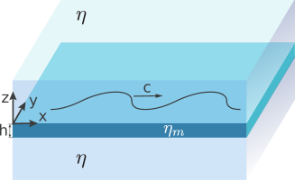
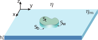
Motivated by recent experimental and theoretical studies of bacteria swimming in biofilms, in freely-suspended thin films (Aranson et al., 2007; Sokolov et al., 2007), and on active proteins mimicking biological swimmers in lipid membranes (Huang et al., 2012), we study here the hydrodynamics of swimming microorganisms in a thin membrane. We treat the membrane as a continuous incompressible viscous fluid film of very small thickness. Flow fields in such a membrane are uniform throughout the thickness of the membrane. In contrast to a thin-film model that involves integration of three-dimensional (3D) hydrodynamic equations across the thickness of the film, our membrane model is intrinsically two-dimensional (2D), in the sense that the motion of molecules within the membrane in the direction normal to the plane of the membrane is forbidden. The membrane is embedded in a 3D fluid of different viscosity. The motion of a swimmer in the membrane generates flows both in the membrane and in the surrounding fluid (see figure 1). While there have been some recent investigations of the hydrodynamics of swimmers in a thin layer of fluid sandwiched between fluids of a different viscosity (Leoni & Liverpool, 2010; Rower et al., 2019), this problem is still largely unexplored.
As was demonstrated by Saffman & Delbrück (1975) and Saffman (1976), the amount of momentum imparted by the membrane to the bulk fluid is controlled by a hydrodynamic length scale, the so-called Saffman length , given by the ratio of the 2D membrane viscosity to the 3D viscosity of the bulk fluid , . If the membrane is perturbed by a localized force (applied in the plane of the membrane) at a point , for distances (measured from ) much smaller than the Saffman length, the effect of the flows in the bulk on the membrane hydrodynamics is negligible. In this region the fluid velocity in the membrane decays slowly (logarithmically) with distance, as in purely 2D fluids. On the other hand, for distances much larger than the Saffman length, the contribution of the bulk fluid to the membrane dynamics is significant, and the membrane flow field decays inversely with the distance, a behavior consistent with 3D dynamics.
Levine & MacKintosh (2002) (LM) derived a Green function for a more general case of viscoelastic membranes. In the case of a purely viscous membrane that we consider here, there is no elastic response of the membrane, and a disturbance caused by a force results in the velocity field alone. The velocity of the membrane at position due to an in-plane, localized force is determined by the LM response tensor ,
| (1) |
Here and are in-plane vectors with components and , respectively (refer also to figure 1 for our choice of the coordinate system). The response function in equation (1) plays the role of the Oseen tensor in D hydrodynamics.
As was shown by LM, the response function may be split into ‘parallel’ and ‘transverse’ contributions. In the component form we have
| (2) |
where , and is the component of the unit vector . In our notation, corresponds to in the LM theory. The scalar functions and are given by
| (3) | |||||
where are Struve functions and are Bessel functions of the second kind (Abramowitz & Stegun, 1965); is the non-dimensionalized distance between the point of application of the force and the point where the membrane velocity response is measured. Both and diverge logarithmically as , while for large we have and
In the small Reynolds number regime the inertia term in the Navier-Stokes equation can be neglected. We assume that the membrane has thickness and choose a coordinate system with the origin at the top surface of the membrane with (therefore, the bottom side of the membrane is at ). The dynamics of the membrane embedded in a bulk fluid is governed by a modified Stokes equation and the incompressibility condition (Saffman, 1976),
| (4) |
where and are the pressure and velocity fields of the membrane. The flows in the membrane set the bulk fluid into motion. The resulting flows in the embedding fluid, in their turn, exert traction on the membrane. Since the membrane is only a few molecular layers thick, the traction due to the bulk fluid produces a flow that is uniform throughout the thickness of the membrane, i.e. the fluid velocity does not depend on for . In equation (4) the coupling between the membrane and the bulk fluid is described by the force per unit volume , with
| (5) |
where is the bulk fluid velocity. The factor of two in equation (4) is due to an equal force acting on the bottom side of the membrane. Equation (4) can be written in a more compact form that we will use later,
| (6) |
where is the stress field of the membrane.
Being inertialess and swimming in the absence of external influences, a swimmer must maintain a zero net force and a zero torque on its body at every time instant,
| (7) | |||||
| (8) |
where the integration is over the surface of the swimmer and is a unit vector normal to the surface and pointing away from the swimmer.
Many microorganisms such as spermatozoa, E. Coli, and Caulobacter crescentus swim by moving thin extensions (flagella) on their bodies. Some critters, like Paramecium, are covered in thousands of short hair-like appendages called cilia and propel themselves through a coordinated beating of these cilia. Since our primary goal is to study how the confinement to the plane of a membrane affects the swimming dynamics of a microorganism (rather than a detailed study of a particular microorganism), we consider here only minimal theoretical models of flagellated and ciliated microorganisms.
In §2 we consider a headless, infinitely long ‘flagellum’ of infinitesimally small thickness propagating planar sinusoidal waves along its body. This is a one-dimensional analog of the Taylor swimmer (Taylor, 1951), an infinite plane in viscous fluid passing transverse sinusoidal waves. We recover Taylor’s result for the swimming velocity in the limiting case of a pure 2D hydrodynamics (the membrane in vacuum). We find that the membrane incompressibility condition imposes a constraint on the fluid dynamics that allows the flagellum to achieve much higher swimming speed than in pure 2D and 3D fluids for large ratios of the wavelength to the Saffman length.
In §3 we study the propulsion of a flagellum of finite length and find its swimming speed and efficiency. In §2 and §3 we apply the boundary-element method (BEM) that two of us have recently developed in work on hydrodynamic interaction of inclusions in freely-suspended smectic films (Qi et al., 2014; Kuriabova et al., 2016; Qi et al., 2017).
In §4 we formulate the Lorentz reciprocal theorem for a quasi-2D fluid and derive an equation for the swimming speed. We discuss the advantage of the method based on the Lorentz reciprocal theorem over the BEM for studying microscopic swimmers with swimming patterns that do not change the overall shape of the swimmers’ bodies (for example, swimmers propagating longitudinal compressive waves along their bodies). As an example of such a critter, we consider a simple model of a two-dimensional ‘squirmer’, a disk with a prescribed tangential velocity along its circumference. We find that unlike its flagellated counterpart, a squirmer does not benefit from the presence of the bulk fluid: its swimming speed is lower than that in a purely 2D fluid.
In §5 we discuss our results and suggest further directions of investigation.
2 Infinitely long flagellum in a quasi-2D membrane
The Taylor swimmer (Taylor, 1951) is an infinite swimming 2D sheet in a 3D viscous fluid that propagates transverse waves of amplitude and wave speed . In a frame moving with the swimming sheet (co-moving frame) the shape of the sheet is described by
| (9) |
where denotes the wave phase.
Taylor showed that the sheet with such a one-dimensional modulation travels, relative to the fluid at infinity, with a speed in the direction opposite to the wave velocity. We consider here a one-dimensional analog of the Taylor swimmer: an infinitely long, infinitesimally thin flagellum confined to the plane of a viscous membrane embedded in bulk fluid (see figure 1) with prescribed motion given by equation (9), with and parametrizing the shape of the flagellum.
A swimming velocity of an infinitely long flagellum is time-independent. Indeed, two snapshots of the waving flagellum taken at the same point on the -axis differ only by a shift along the -axis. Thus, a temporal shift at a fixed point is equivalent to a spatial displacement along the flagellum. A swimmer moving as a whole has the same translational velocity along its entire length. The swimming velocity, being invariant with respect to translations along the -axis must be invariant with respect to translations in time as well. Therefore, we can calculate the swimming speed for a single time instant and set in equation (9).
As in (Taylor, 1951) we consider the case of an inextensible flagellum. In order to calculate the portion of the swimmer’s velocity due to its distortion, we calculate the position of a material point of the flagellum as a function of time. In a frame moving with the wave (with speed relative to the co-moving frame) the shape of the flagellum does not change. The Cartesian coordinates for this frame are , where . In this reference frame a material particle of the flagellum travels a distance equal to the arclength of the flagellum spanned by one (linear) wavelength during one period of oscillation ,
| (10) |
We will call the arcwise wavelength. The material particle’s speed is, therefore,
| (11) | |||||
| (12) |
To determine the position of a material particle of the flagelleum, we define the material coordinate to be the arclength coordinate of a material point at . In the frame in which the nodes of the wave are fixed, arclength is related to the Cartesian coordinate by
| (13) | |||||
| (14) |
Reverting the series leads to
| (15) |
Using and leads to the position of the material point labeled by as a function of time :
| (16) | |||||
| (17) | |||||
In the co-moving frame the components of a material particle’s velocity are given by
| (18) |
For an arbitrary value of , the material particle’s velocity can be calculated numerically using
| (19) | |||||
| (20) |
with . The total velocity of a material particle relative to the fluid at infinity (for ) is the sum of the surface disturbance and swimming velocities, .
The linearity of Stokes equations allows us to model the fluid velocity field in the membrane as a superposition of fluid velocities due to a (yet unknown) force density along the flagellum:
| (21) |
where the integration is along the (infinite) contour of the flagellum.
The spatial periodicity of the flagellum modulation implies the invariance of the flow field and the force density in equation (21) under translations along the -axis by an integer multiple of the wavelength . Defining , for all integers , the integration on the RHS of equation (21) can be reduced to integration over a single wavelength. We impose a no-slip boundary condition on the surface of the flagellum by setting the fluid velocity equal to the velocity of the material point on the flagellum,
| (22) |
where and indicate the points on the flagellum that belong to a one-wavelength ‘window’ and . The surface disturbance velocity on the LHS of equation (22) is given by equation (18).
To close the system of equations for the force density and the swimming velocity , we also require the net force on the flagellum be equal to zero,
| (23) |
We solved equations (22) and (23) numerically in Matlab by splitting the integration path into straight-line segments of equal length and replacing the line integrals in equations (22) and (23) by summation over the segments,
| (24) |
| (25) |
In equations (24) and (25) are the coordinates of the segments’ midpoints. In equation (24) we introduced the truncation parameter for the infinite sum over the wavelengths.
For a starting value of parameter (usually ), we ran computations for five different values of parameter in the range – and then extrapolated our results for the swimming velocity to (). We then gradually increased the value of and repeated the computations until the solution for converged, showing changes smaller than with further increase of the number of terms in the sum over . The computations required increasingly more terms in the sum over for large amplitudes () and large Saffman lengths () due to strong long-range hydrodynamic interactions between segments of the flagellum in this (nearly 2D) regime, and correspondingly large contribution to the flow field by the forces separated by multiple wavelengths along the flagellum.
We paid special attention to the diagonal term with and in equation (24). This term gives the fluid velocity in the close proximity of a localized force . The response tensor diverges due to logarithmic singularities in the functions and in the limit [see equations (3) and (1)]. In the close proximity of a localized force the fluid velocity is parallel to the force, and is, therefore, determined by the parallel component of the response function . We expanded about and performed integration analytically over in the vicinity of . Therefore, for the diagonal term on the RHS of equation (24), which we denote as , we have
| (26) | |||||
where is the Euler constant.
Our computations confirm that an infinitely long flagellum has a non-vanishing component of the swimming velocity only along the -axis, as expected by symmetry. In figure 2 we plot the swimming speed as a function of the dimensionless amplitude for a range of wavelengths scaled by the Saffman length. In the limit of pure 2D hydrodynamics, which corresponds to large Saffman lengths (and small scaled wavelengths, ), the energy dissipation occurs primarily in the membrane, and the membrane’s viscous drag on the flagellum makes the main contribution to the flagellum’s propulsion. In this limit, our computations are in good agreement with the 2D problem of the Taylor swimming sheet, as expected because a Taylor ‘string’ in a thin very viscous membrane is equivalent to the Taylor sheet in 3D bulk fluid. For small amplitudes (), we recover Taylor’s leading order perturbative solution . For larger amplitudes (and ), our calculated swimming speed is in agreement with recent analytic and computational results of Sauzade and coworkers (Sauzade et al., 2011).
In figure 2 the black dashed curve corresponds to a flagellum swimming in a pure 2D membrane (no bulk fluid surrounding the membrane). We briefly outline our computations for this limiting case in Appendix A. The computations are similar to the boundary integral approach demonstrated in (Sauzade et al., 2011) with the only difference that we neglected the double layer potential contribution. The solid black curve in figure 2 corresponds to the local drag theory for an infinitely long flagellum passing waves of moderately large amplitudes in a 3D unbounded fluid (Gray & Hancock, 1955).
As can be seen in figure 2, our BEM computations predict that for wavelengths larger than the Saffman length () the swimming speed in a quasi-2D membrane exceeds that in purely 2D and 3D fluids. For qualitative explanation of this result we compare our BEM computations with the local drag model of Gray & Hancock (1955). In the local drag approximation, one assumes that the viscous drag force on a small segment of the flagellum is proportional to the segment’s velocity, and the total drag on the swimmer is a sum over these local drag forces. Thus, the local drag approximation does not explicitly take into account the long-range hydrodynamic interactions between distant segments of the flagellum. The local drag forces for the motion of a rod-like segment parallel and perpendicular to its geometrical axis are given by and , respectively, with the drag coefficients and .
We expect our BEM results to be in qualitative agreement with the local drag approximation in the limit of and . For small amplitudes the segments of an inextensible flagellum separated by large contour distances () do not come too close to each other, and for the wavelengths larger than the Saffman length the spatial decay of the flow field is faster (), in comparison with slower (logarithmic) decay rate for . Thus in the regime of and , the cooperativity effect between distant segments of the flagellum is expected to be small. Gray & Hancock (1955) obtained the swimming velocity of an infinitely long and thin flagellum to the leading order of amplitude ,
| (27) |
In 3D, the ratio of the drag coefficients for an infinitely thin rod is . For inclusions in quasi-2D membranes, the ratio depends on the Saffman length. In the inset of figure 2 we plot our BEM results for as a function of . According to equation 27, should give us an estimate for the local drag anisotropy. For the plot in the inset we chose a small amplitude , when the comparison with the local drag calculation of Gray and Hancock is justified. As can be seen in the inset of figure 2, the effective ratio grows logarithmically with for .
This result is in qualitative agreement with the work of Levine and collaborators (Levine et al., 2004), some of which we summarize here. Levine et al. studied the drag coefficients for a rod-like inclusion of length moving in a quasi-2D membrane, and showed that for rod-like inclusions of lengths smaller than the Saffman length (), where the viscous dissipation occurs primarily in the membrane, the dependence of the drag coefficients on the size and orientation of the rod is weak: . For longer rods with , the dissipation is governed by the 3D fluid surrounding the membrane, and the drag coefficients show a stronger dependence on the size of the rods. Levine et al. found that the drag coefficient for a thin rod in a quasi-2D membrane is qualitatively similar to that in 3D and is given by
| (28) |
However, the dependence of on in a quasi-2D membrane is very different from that in 3D:
| (29) |
depends on linearly, without the logarithmic factor in the denominator. The linear dependence of on indicates the local character of the drag and the effective absence of hydrodynamic interactions between different sections of the rod.
As emphasized by Levine et al. (2004), this behavior of arises from the incompressibility of the membrane, , where the symbol denotes differentiation ‘in-plane’ and the components of the velocity field in the plane. In the case of a rod moving perpendicular to its long axis in a 3D fluid, the fluid can flow past the rod by moving over and under it. In this flow pattern, the in-plane part of the incompressibility condition does not vanish: . A 2D version of such a flow (its projection on the -plane) is impossible due to the membrane incompressibility. In a quasi-2D membrane, the fluid moves the long way around the rod, and the flow extends over distances comparable to the largest rod dimension . The membrane incompressibility constraint only affects the perpendicular drag on a filament. A segment of filament being dragged parallel to its long axis does not produce divergent flows in a simple fluid, and thus the flow character is unchanged by the presence of a membrane.
Therefore, for long wavelengths (), the membrane incompressibility is expected to lead to a logarithmic growth of the flagellum’s effective drag anisotropy, . An organism that relies on the drag anisotropy for propulsion would achieve greater swimming speeds in a quasi-2D membrane than in pure 2D or 3D fluids, as is confirmed by our BEM computations.
3 Finite length flagellum in a quasi-2D membrane
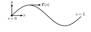
We also applied the BEM to the case of an inextensible, headless, infinitely thin flagellum of finite length. As in the case of an infinitely long flagellum, the motion of the swimmer is prescribed by a sinusoidal modulation, . Here is the arc length along the flagellum measured from the flagellum’s hypothetical ‘head’ and is the initial phase. At every time instant, the shape of the flagellum is described by the curve , where (see figure 3). The unit tangent to the curve is .
In the frame of the flagellum, a material point at position moves with velocity . As was demonstrated by Higdon (1979), in the case of transverse waves propagating along the flagellum, the material particle’s velocity can be calculated in a different manner. In a reference frame moving with the wave, the shape of the flagellum is given by , where is the arcwise speed that we introduced in equation (11). Following Higdon, we note that
| (30) |
where is the arcwise wavelength (see equation (10)) and is the linear wavelength. The tangential vectors are identical in the body and wave frames since the wave frame simply translates with respect to the body frame and does not undergo rotation. Thus, . The velocity of a material particle at in the wave frame is calculated as . The velocity of the ‘head’ in the wave frame is . Therefore, the wave frame translates with respect to the body frame with velocity . Therefore, we can calculate the velocity of the material point in the body frame as
| (31) |
The material velocity with respect to the fluid at infinity is then
| (32) |
where and are the translational and angular velocities of the flagellum.
Similarly to our treatment of an infinitely long flagellum in §2, we model the fluid velocity due to the flagellum’s motion as a linear superposition of velocities due to a force density (see equation (21)). Now the path of integration stands for the curve describing the instantaneous shape of the flagellum. The instantaneous swimming and angular velocities and the force density are calculated from the coupled integral equations for a no-slip boundary condition on the surface of the flagellum and the requirements of zero net force and torque on the flagellum,
| (33) |
| (34) | |||||
| (35) |
where and .
Similar to the approach discussed in §2, we solved the discretized version of these equations for the instantaneous velocities , and the force density . We normally calculated the angular and swimming velocities for about 60–80 snapshots per one period of oscillation and averaged them over one cycle of motion, and , where is the rotation operator that transforms the swimming velocity vector to the initial coordinate system , which is motionless with respect to the fluid at infinity, and is the number of snapshots per one period.

During one cycle of motion, a flagellum of finite size moves in a tortuous fashion that involves pitching (rotation of the swimmer’s centerline with respect to the initial direction of wave propagation) and drifting (motion of the flagellum’s center of mass perpendicular to the net swimming direction), see figure 4.
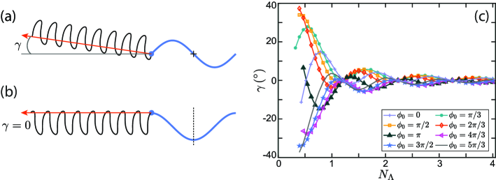
Our computations predict that , and a flagellum of finite size swims in a straight line at an angle with respect to -axis, where . The magnitude and sign of depend on the flagellum’s contour length, the wave amplitude and the phase constant . For particular values of , a flagellum of a given contour length can assume an even or odd configuration at time . In the even configuration (as illustrated in figure 5b) the flagellum has reflection symmetry with respect to the vertical dashed line that passes through the flagellum’s center of mass. In the odd configuration the shape of the flagellum has point symmetry about the center of the flagellum (marked by cross hairs in figure 5a).
Koehler et al. (2012), in work on the swimming of finite-length flagella in a Newtonian 3D fluid, used symmetry arguments to prove that a flagellum that starts its motion from an even configuration swims along its centerline in the direction opposite to initial wave propagation, and does not drift away from the -direction. Koehler et al. (2012) pointed out that the mirror reflection about the vertical line is equivalent to the time reversal, with the time-reversed swimming velocity . Therefore, the instantaneous swimming velocity in an even configuration must be identical to the mirror image of the time-reversed velocity. This condition requires the - component of the swimming velocity be equal to zero. Thus, a flagellum starting its motion from an even configuration, has vanishing mean drift over one cycle of motion. A flagellum starting its motion in an odd configuration, will reach an even configuration after a quarter of a period. The reorientation angle acquired by the flagellum by determines the flagellum’s swimming direction. The reorientation angle for a flagellum starting its motion in an odd configuration is the largest since it takes the longest amount of time for such a flagellum to reach an even configuration. In figure 5 we plot as a function of the flagellum’s contour length for various values of the phase constant . A similar swimming pattern was reported by Peng et al. (2016) in the work on flagella locomotion in granular media.
In figure 6a we plot the swimming speed averaged over one period of oscillations, , as a function of a dimensionless parameter for the flagellum contour length equal to one arcwise wavelength, . Two competing mechanisms influence the swimming speed of the flagellum. On the one hand, larger values of correspond to steeper angles between the flagellum and the direction of wave propagation and, therefore, a stronger propulsion force. On the other hand, for larger values the segments of the flagellum come closer to each other. The hydrodynamic interactions between the segments tend to slow down the swimmer. The hydrodynamic interactions are stronger in the limiting case of 2D hydrodynamics (small ratios) due to a slow, logarithmic spatial decay rate of the flow field. In the opposite limit of large ratios, our calculations do not reproduce Higdon’s results for the swimming speed in a purely 3D fluid (Higdon, 1979). Being qualitatively similar to Higdon’s prediction, our calculations show much larger swimming speeds for . As we discussed at the end of §2, the incompressibility of the membrane sets a constraint on the fluid dynamics that leads to an effective drag anisotropy that grows logarithmically as a function of for . The enhanced drag anisotropy in a quasi-2D membrane is responsible for larger swimming speeds in quasi-2D membranes (in comparison with pure 2D or 3D fluids).
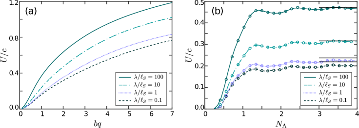
In figure 6b we plot the swimming speed as a function of the scaled flagellum length for . For the flagellum performs large yawing motion that is inefficient for swimming (see figure 4a). For larger values of the long-range hydrodynamic interactions taper off the growth of the swimming speed, and the speed approaches the values found for an infinitely long flagellum (shown as dotted black horizontal lines in figure 6b). The ‘bumps’ in the curves reflect smaller yawing of the flagellum for some values of .
To find the flagellum motion that is optimal in terms of the power consumption, we calculated the swimming efficiency. As discussed in (Koehler et al., 2012), there are multiple efficiency metrics. Here we calculated the efficiency as the ratio of the power required to pull the flagellum through the fluid at its average swimming speed, , to the average power consumed by the swimmer over one period of motion,
| (36) |
Here is the flagellum mobility for the translational motion along the direction of wave propagation, averaged over one period. The average power consumption is
| (37) |
We calculated the mobility and the power consumption numerically using the BEM.
Our calculated flagellum efficiency is in qualitative agreement with Higdon (1979). In figure 7a we plot the efficiency as a function of the amplitude for a few values of the scaled wavelength for a flagellum of length . For smaller values of the segments of the flagellum have small angles with respect to the direction of wave propagation and produce a weak thrust. For larger values of the flagellum ‘shrinks’ along the -axis, and the stronger interference between the segments of the flagellum leads to a decrease in efficiency. The efficiency increases with due to the reduced role of long-range hydrodynamics on length scales exceeding the Saffman length . The maximum efficiency falls at 1.4 – 1.8.
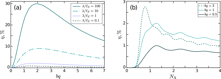
In figure 7b we plot the efficiency as a function of the flagellum length for a wavelength . For small values of the swimming of the flagellum is inefficient due to an excessive yawing motion and a weak overall thrust (see figure 4a). The efficiency reaches a maximum at = 0.8 – 1.4 and then decreases with further growth of due to interference between the crests of the flagellum. The interference is stronger for larger amplitudes since the crests are closer to each other, and the efficiency drops off more abruptly from its optimal value for larger values of . The secondary maxima correspond to a smaller yawing and larger propulsion for various values of . Figure 4 demonstrates that the flagellum travels a considerable distance along the -axis while making moderate overall progress along the -axis.
In the following section we discuss an alternative computational approach to finding the swimming velocities using the Lorentz reciprocal theorem.
4 Lorentz reciprocal theorem for a quasi-2D membrane
Finding the analytical solution for the swimming velocity can be a daunting task. One of the major difficulties is that one needs to solve Stokes equations with time dependent no-slip boundary conditions on the surface of the swimmer. Stone & Samuel (1996) offered an elegant way to find the swimming velocity using the Lorentz reciprocal theorem (LRT) (Happel & Brenner, 1965). For a fluid in 3D the Lorentz reciprocal theorem states that if there are two solutions to Stokes equations and the incompressibility condition with the velocity fields and the stress tensors and , respectively, that satisfy the same boundary conditions at infinity, than for a volume of fluid bounded by surface , we have
| (38) |
where is the outward normal to the surface .
Here we formulate the LRT approach for a finite swimmer confined to a quasi-2D membrane. Let and be the membrane velocity and the stress fields for the swimming problem. These velocity and stress fields are solutions of the Stokes equations and the incompressibility condition, equation (4). They also satisfy the conditions of zero net force and torque on the swimming body, equations (7) and (8). For the reciprocal solution of equation (4) we choose the membrane velocity and stress fields due to an inactive object of the same shape as the swimmer and being dragged as a solid body with constant translational velocity .
When the condition is relaxed (see equation (6)), a more general form of the Lorentz reciprocal theorem is (Kim & Karrila, 1991)
| (39) |
where is the swimmer’s volume bounded by the surface . Here we treat the volume occupied by the swimmer as being equivalent to the fluid domain of the same shape as the swimmer’s and having the same velocity distribution as that of the material particles of the swimmer.
Let us consider the first term on the LHS of equation (39):
| (40) |
where we took into account that is a constant vector at the surface of the domain (uniform translation). Also, since does not have - components, only on the curvy wall of the domain, (see figure 8), will make a non-zero contribution.
Taking into account equation (6), the second term on the LHS of equation (39) can be rearranged as
| (41) |
where we take into account that the traction forces due to the fluid flows in the surrounding fluid act on the flat sides of the domain (see equation (6) and figure 8), and . Therefore, the LHS of equation (39) becomes:
| (42) |
where is the net force on the swimmer and is equal to zero.
Similarly, for the terms on the RHS of equation (39) we have
| (43) | |||||
where in the last line of equation (43) we merged two terms into one integral over the total surface of the swimmer, and denotes an elementary traction force on the inactive ‘swimmer’ being dragged with constant velocity. Thus, the Lorentz reciprocal relation, equation (39), assumes a compact form,
| (44) |
Decomposing the surface velocity of the swimmer into the translational and the surface disturbance velocities, , we rewrite the Lorentz reciprocal relation in the form
| (45) |
similar to the equation derived by Stone & Samuel (1996) for a swimmer in a 3D fluid. In equation (45) the integration is performed over the instantaneous surface area of the swimmer. The generalization of (45) for the motion that involves rotation is
| (46) |
where is the torque applied to the inactive inclusion and is the swimmer’s angular velocity.
The Lorentz reciprocal relation, equation (46), is particularly useful for computation of the swimmer’s translational and rotational velocities, and , when the stress tensor of the reciprocal problem (motion of an inactive body) is known. Unfortunately, it is also difficult to solve the reciprocal problem analytically for an inclusion of an arbitrary shape in a quasi-2D membrane, since the coupling with the bulk fluid makes the problem essentially three-dimensional. When the reciprocal solution is not available, equation (46) can serve as an alternative computational path for finding the swimming velocity.
As a test of equation (46), we found the swimming velocities of a finite inextensible flagellum as described in §3. We solved the reciprocal problem numerically by finding the force densities for the uniform rotation of the flagellum about the -axis and for the translational motion of the flagellum along the - and - axes for multiple flagellum conformations corresponding to various time instants of the swimming cycle. We then solved the resulting system of three equations (46) for the instantaneous angular velocity and - and - components of the translational velocity and found the average swimmer’s speed over one period of oscillations. In figure 6b circles superimposed on the curves show the swimming velocities obtained using the Lorentz equation (46).
4.1 The two-dimensional squirmer example
The Lorentz reciprocal theorem can significantly simplify computations in the case of tangential deformations of the swimmer’s body, when the overall shape of the critter remains unchanged. In this case the reciprocal problem can be solved for a single time instant, and the instantaneous swimming velocity can then be found from equation (46) by plugging in the time-dependent surface disturbance velocity .
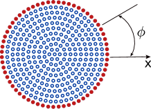
As an example, we consider a two-dimensional version of a squirmer, a critter that propels itself by beating its multiple hair-like appendages (cilia) in a periodic fashion. The periodic motion of the cilia carpet can be modeled by prescribing a velocity field on the surface of the squirmer. In a minimal model of a 2D squirmer, a disk-like body of radius is propelled due to a tangential disturbance velocity on the disk circumference (see figure 9), where and are constants (Blake, 1971; Papavassiliou & Alexander, 2015). The material points in the interior of the disk are motionless in the frame of the squirmer. When the constants and have the same sign, they describe a contractile swimmer. Otherwise, the model corresponds to an extensile swimmer.
In the limit of the reciprocal problem for a disk was solved by Saffman (1976) in the studies related to the Stokes paradox and a particle mobility in a quasi-2D fluid. In Appendix B we outline calculations for the swimming velocity of the squirmer in the limit using Saffman’s solution for the reciprocal stress tensor . The LRT reproduces the known swimming speed , for a 2D squirmer in the limiting case of pure 2D hydrodynamics.
Since the analytical solution for the reciprocal problem for a disk of arbitrary radius is not readily available, we found the reciprocal stress numerically by adopting the method of regularized Stokeslets (RS) for a quasi-2D membrane developed by Camley & Brown (2013) in their work on mobility of inclusions in a quasi-2D membrane. In (Camley & Brown, 2013) the flow field due to a moving inclusion is modeled as a superposition of the flow fields due to point-like forces (blobs) tiling the disk area (see figure 9),
| (47) |
where ; is the total number of blobs; is the in-plane coordinate of the -th blob; is the Levine-MacKintosh response function (see equations 2); and is the unknown force distribution.
In the reciprocal problem the disk is being pulled through the membrane as a solid object with some given velocity . The force distribution over the blobs is found by imposing a no-slip boundary condition on each blob,
| (48) |
Due to the squirmer’s reflection symmetry about the -axis, the rotational motion of the squirmer in an unbounded domain is ruled out, and the swimming velocity can be found from the discretized version of equation (45),
| (49) |
The summation on the RHS of equation (49) is carried out only over the blobs on the squirmer’s circumference since the inner blobs are motionless in the critter’s frame.
In the RS method the logarithmic singularity of the membrane response functions for is eliminated by the regularization (smoothing) process that involves integration of the response function over the blob envelope function centered at . Camley & Brown (2013) selected a Gaussian function for the regularization. The width of the Gaussian is controlled by an auxiliary parameter . Camley and Brown set , where is the distance between the centers of adjacent blobs, calculated the inclusion mobilities for several values of in the range –, and extrapolated the results to the limit . While the numerical calculations for the inclusion mobilities are only weakly dependent on the choice of in our case of a swimming squirmer, the swimming velocities are more sensitive to the choice of the regularization parameter , since it effectively determines the thickness of the squirmer’s deforming outer ring and its permeability, and therefore becomes a physical parameter.
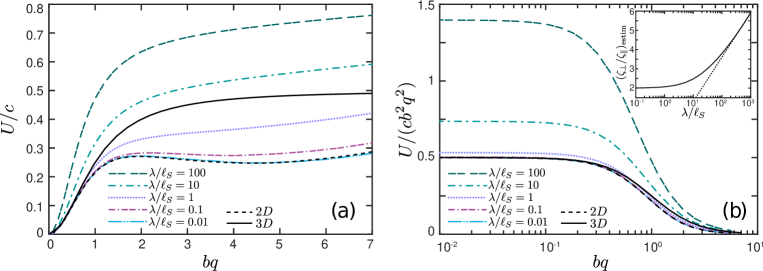
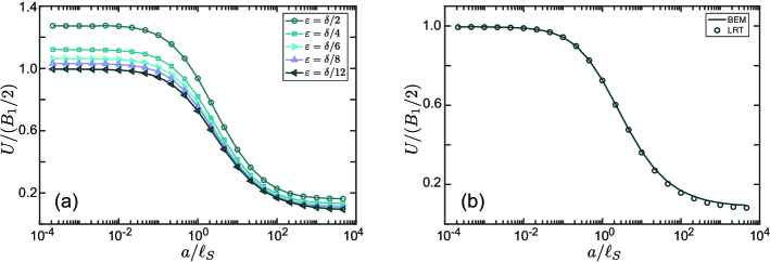
In figure 10a we plot the LRT results for the scaled swimming speed of a squirmer, , as a function of the squirmer radius for several values of parameter . As in Camley & Brown (2013), for a selected dependence of on (e.g. ), we calculated the swimming speed for a range of ’s and extrapolated it to . As can be seen in figure 10a, the regularization parameter gives the swimming velocity that is close to the known value of in the limiting case of a pure 2D membrane (membrane in vacuum). Our calculations also show that the scaled swimming velocity is independent of the ratio .
In figure 10b we compare the results of calculations for the swimming speed obtained within the LRT and the BEM for . For the direct BEM calculation of the swimming speed and the force distribution we solved simultaneously the equations that impose no-slip boundary conditions and a zero net force on the swimmer,
| (50) | |||||
| (51) | |||||
| (52) |
As can be observed in figure 10b, the squirmer swimming velocity decreases with an increase of ratio. Larger values of correspond to a larger viscosity of the fluid embedding the membrane, which leads to a stronger traction on the ‘back’ and ‘belly’ of the critter.
5 Conclusion
We have studied analytically and computationally the locomotion of microscopic organisms confined to a plane of a thin fluid membrane embedded in a bulk fluid of different viscosity. In our model the membrane is sufficiently thin, with material particles moving only in the plane of the membrane (the motion in the perpendicular direction is forbidden).
The presence of the bulk fluid allows the introduction of a hydrodynamic length scale, the Saffman length, that controls the energy exchange between the membrane and the surrounding fluid. By varying the Saffman length, we make our model continuously vary between a pure 2D system (large Saffman length) and a quasi-2D system (small Saffman length). The hydrodynamic flows in the quasi-2D membrane have features of both 3D and 2D hydrodynamics. We show that a flagellated swimmer in a viscous film (Saffman length smaller than swimmer characteristic length scale) swims faster than the same swimmer in a 3D fluid. The speedup comes from the effectively larger perpendicular drag coefficient, which arises from the incompressibility of the membrane. On the other hand, a circular squirmer, whose propulsion mechanism does not employ the local drag anisotropy, slows down for smaller Saffman lengths (in comparison with the squirmer’s radius).
The coupling of the membrane with the bulk fluid makes the problem three-dimensional and quite difficult for analytical treatment. We developed numerical schemes based on the boundary element method and the Lorentz reciprocal theorem. We show how the Lorentz reciprocal theorem can be used to simplify the computation of swimming speed, especially for swimmers such as the squirmer that do not change shape during a stroke.
While we considered the minimal models of a flagellated swimmer and of a squirmer, our approach can be generalized to other swimmers’ geometries and swimming stokes.
Acknowledgements We thank M. Moelter for helpful discussions. This work has been supported by a Cottrell College Science Award (TK) and National Science Foundation Grant No. 1437195 (TRP). (CA) gratefully acknowledges support from a Frost Undergraduate Student Research Award.
Appendix A Infinitely long flagellum in 2D fluid
In the 2D limit (membrane in vacuum) the system of equations (24) becomes
| (53) |
where is a 2D periodic Stokeslet,
| (54) |
with , and . In equations (53) and (54) all variables are dimensional. The periodic Stokeslets can be expressed in closed form (Sauzade et al., 2011; Pozrikidis, 1987) using the analytic formula for the summation,
| (55) |
The components of the periodic stokeslet can be found as
| (56) | |||||
| (57) | |||||
| (58) |
where , indicate the derivatives of with respect to and respectively. Similar to our treatment of the diagonal terms in equation (26) we eliminate the logarithmic singularity by analytic integration,
| (59) |
Appendix B Swimming velocity of a squirmer in the 2D limit
We consider a tangential squirmer with a prescribed surface velocity of the form
| (60) |
with free parameters and . Since the disturbance velocity has only a - component, the RHS of equation (46) becomes:
| (61) | |||||
where we took into account , where is the thickness of the membrane. Therefore, equation (46) becomes
| (62) |
The membrane stress tensor element is determined as
| (63) |
For a special case of Saffman (1976) found
| (64) | |||||
| (65) |
with
| (66) |
Here is the Euler constant.
References
- Abramowitz & Stegun (1965) Abramowitz, M. & Stegun, I. 1965 Handbook of Mathematical Functions. Dover Publications.
- Aranson et al. (2007) Aranson, I. S., Sokolov, A., Kessler, J. O. & Goldstein, R. E. 2007 Model for dynamical coherence in thin films of self-propelled microorganisms. Phys. Rev. E 75, 040901.
- Berke et al. (2008) Berke, A. P., Turner, L., Berg, H. C. & Lauga, E. 2008 Hydrodynamic attraction of swimming microorganisms by surfaces. Phys. Rev. Lett. 101, 038102.
- Blake (1971) Blake, J. R. 1971 A spherical envelope approach to ciliary propulsion. J. Fluid Mech. 46 (1), 199–208.
- Camley & Brown (2013) Camley, B. A. & Brown, L. H. 2013 Diffusion of complex objects embedded in free and supported lipid bilayer membranes: role of shape anisotropy and leaflet structure. Soft Matter 9, 4767.
- Childress (1981) Childress, S. 1981 Mechanics of Swimming and Flying. Cambridge University Press.
- Crowdy & Or (2010) Crowdy, D. G. & Or, Y. 2010 Two-dimensional point singularity model of a low-Reynolds-number swimmer near a wall. Phys. Rev. E 81, 036313.
- Di Leonardo et al. (2011) Di Leonardo, R., Dell’Arciprete, D., Angelani, L. & Iebba, V. 2011 Swimming with an image. Phys. Rev. Lett. 106, 038101.
- Drescher et al. (2009) Drescher, K., Leptos, K. C., Tuval, I., Ishikawa, T., Pedley, T. J. & Goldstein, R. E. 2009 Dancing volvox: Hydrodynamic bound states of swimming algae. Phys. Rev. Lett. 102, 168101.
- Gray & Hancock (1955) Gray, J. & Hancock, G. J. 1955 The propulsion of sea-urchin spermatozoa. J. Exp. Biol. 32 (4), 802–814.
- Guasto et al. (2010) Guasto, J. S., Johnson, K. A. & Gollub, J. P. 2010 Oscillatory flows induced by microorganisms swimming in two dimensions. Phys. Rev. Lett. 105, 168102.
- Happel & Brenner (1965) Happel, J. R. & Brenner, H. 1965 Low Reynolds number hydrodynamics: with special applications to particulate media. Martinus Nijhoff.
- Higdon (1979) Higdon, J. J. L. 1979 A hydrodynamic analysis of flagellar propulsion. J. Fluid Mech. 90 (4), 685–711.
- Huang et al. (2012) Huang, M.-J., Chen, H.-Y. & Mikhailov, A. S. 2012 Nano-swimmers in biological membranes and propulsion hydrodynamics in two dimensions. Eur. Phys. J. E 35 (11), 119.
- Ishimoto et al. (2016) Ishimoto, K., Cosson, J. & Gaffney, E. A. 2016 A simulation study of sperm motility hydrodynamics near fish eggs and spheres. J. Theor. Biol. 389, 187–197.
- Kim & Karrila (1991) Kim, S. & Karrila, J. S. 1991 Microhydrodynamics: Principles and Selected Applications. Boston, MA: Butterworth-Heinemann.
- Koehler et al. (2012) Koehler, S., Spoor, T. & Tilley, B. S. 2012 Pitching, bobbing, and performance metrics for undulating finite-length swimming filaments. Phys. Fluids 24 (9), 091901.
- Kuriabova et al. (2016) Kuriabova, T., Powers, T. R., Qi, Z., Goldfain, A., Park, C. Soo, Glaser, M. A., Maclennan, J. E. & Clark, N. A. 2016 Hydrodynamic interactions in freely suspended liquid crystal films. Phys. Rev. E 94, 052701.
- Lambert et al. (2013) Lambert, R. A., Picano, F., Breugem, W.-P. & Brandt, L. 2013 Active suspensions in thin films: nutrient uptake and swimmer motion. J. Fluid Mech. 733, 528–557.
- Lauga et al. (2006) Lauga, E., DiLuzio, W. R., Whitesides, G. M. & Stone, H. A. 2006 Swimming in Circles: Motion of Bacteria near Solid Boundaries. Biophys. J. 90 (2), 400–412.
- Lauga & Powers (2009) Lauga, E. & Powers, T. R. 2009 The hydrodynamics of swimming microorganisms. Rep. Prog. Phys. 72 (9), 096601.
- Leoni & Liverpool (2010) Leoni, M. & Liverpool, T. B. 2010 Swimmers in thin films: from swarming to hydrodynamic instabilities. Phys. Rev. Lett. 105, 238102.
- Levine et al. (2004) Levine, A. J., Liverpool, T. B. & MacKintosh, F. C. 2004 Mobility of extended bodies in viscous films and membranes. Phys. Rev. E 69, 021503.
- Levine & MacKintosh (2002) Levine, A. J. & MacKintosh, F. C. 2002 Dynamics of viscoelastic membranes. Phys. Rev. E 66, 061606.
- Li et al. (2011) Li, G., Bensson, J., Nisimova, L., Munger, D., Mahautmr, P., Tang, J. X., Maxey, M. R. & Brun, Y. V. 2011 Accumulation of swimming bacteria near a solid surface. Phys. Rev. E 84, 041932.
- Li & Tang (2009) Li, G. & Tang, J. X. 2009 Accumulation of microswimmers near a surface mediated by collision and rotational brownian motion. Phys. Rev. Lett. 103, 078101.
- Lopez & Lauga (2014) Lopez, D. & Lauga, E. 2014 Dynamics of swimming bacteria at complex interfaces. Phys. Fluids 26 (7), 071902.
- Masoud & Stone (2014) Masoud, H. & Stone, H. A. 2014 A reciprocal theorem for marangoni propulsion. J. Fluid Mech. 741, 7.
- Mathijssen et al. (2016a) Mathijssen, A. J. T. M., Doostmohammadi, A., Yeomans, J. M. & Shendruk, T. N. 2016a Hotspots of boundary accumulation: dynamics and statistics of micro-swimmers in flowing films. J. R. Soc. Interface 13 (115), 20150936.
- Mathijssen et al. (2016b) Mathijssen, A. J. T. M., Doostmohammadi, A., Yeomans, J. M. & Shendruk, T. N. 2016b Hydrodynamics of micro-swimmers in films. J. Fluid Mech. 806, 35–70.
- Molaei et al. (2014) Molaei, M., Barry, M., Stocker, R. & Sheng, J. 2014 Failed escape: Solid surfaces prevent tumbling of Escherichia coli. Phys. Rev. Lett. 113, 068103.
- Or & Murray (2009) Or, Y. & Murray, R. M. 2009 Dynamics and stability of a class of low Reynolds number swimmers near a wall. Phys. Rev. E 79, 045302.
- Or et al. (2011) Or, Y., Zhang, S. & Murray, R. M. 2011 Dynamics and stability of low-Reynolds-number swimming near a wall. SIAM J. on Applied Dynamical Systems 10 (3), 1013–29.
- Ota et al. (2018) Ota, Y., Hosaka, Y., Yasuda, K. & Komura, S. 2018 Three-disk microswimmer in a supported fluid membrane. Phys. Rev. E 97, 052612.
- Papavassiliou & Alexander (2015) Papavassiliou, D. & Alexander, G. P. 2015 The many-body reciprocal theorem and swimmer hydrodynamics. EPL (Europhys. Lett.) 110 (4), 44001.
- Pedley & Kessler (1987) Pedley, T. J. & Kessler, J. O. 1987 The orientation of spheroidal microorganisms swimming in a flow field. Proc. R. Soc. Lond. B 231 (1262), 47–70.
- Peng et al. (2016) Peng, Z., Pak, O. S. & Elfring, G. J. 2016 Characteristics of undulatory locomotion in granular media. Phys. Fluids 28 (3), 031901.
- Pozrikidis (1987) Pozrikidis, C. 1987 Creeping flow in two-dimensional channels. J. Fluid Mech. 180, 495–514.
- Purcell (1977) Purcell, E. M. 1977 Life at low Reynolds number. Am. J. Phys. 45 (1), 3–11.
- Qi et al. (2017) Qi, Z., Ferguson, K., Sechrest, Y., Munsat, T., Park, C. S., Glaser, M. A., Maclennan, J. E., Clark, N. A., Kuriabova, T. & Powers, T. R. 2017 Active microrheology of smectic membranes. Phys. Rev. E 95, 022702.
- Qi et al. (2014) Qi, Z., Nguyen, Z. H., Park, C. S., Glaser, M. A., Maclennan, J. E., Clark, N. A., Kuriabova, T. & Powers, T. R. 2014 Mutual diffusion of inclusions in freely suspended smectic liquid crystal films. Phys. Rev. Lett. 113, 128304.
- Rower et al. (2019) Rower, D. A., Padidar, M. & Atzberger, P. J. 2019 Surface fluctuating hydrodynamics methods for the drift-diffusion dynamics of particles and microstructures within curved fluid interfaces. ArXiv:1906.01146.
- Saffman (1976) Saffman, P. G. 1976 Brownian motion in thin sheets of viscous fluid. J. Fluid Mech. 73, 593.
- Saffman & Delbrück (1975) Saffman, P. G. & Delbrück, M. 1975 Brownian motion in biological membranes. Proc. Natl. Acad. Sci. USA 72, 3111.
- Sauzade et al. (2011) Sauzade, M., Elfring, G. J. & Lauga, E. 2011 Taylor’s swimming sheet: Analysis and improvement of the perturbation series. Physica D 240 (20), 1567–1573.
- Sokolov et al. (2007) Sokolov, A., Aranson, I. S., Kessler, J. O. & Goldstein, R. E. 2007 Concentration dependence of the collective dynamics of swimming bacteria. Phys. Rev. Lett. 98, 158102.
- Spagnolie & Lauga (2012) Spagnolie, S. E. & Lauga, E. 2012 Hydrodynamics of self-propulsion near a boundary: predictions and accuracy of far-field approximations. J. Fluid Mech. 700, 105–147.
- Stone & Masoud (2015) Stone, H. A. & Masoud, H. 2015 Mobility of membrane-trapped particles. J. Fluid Mech. 781, 494–505.
- Stone & Samuel (1996) Stone, H. A. & Samuel, A. D. T. 1996 Propulsion of microorganisms by surface distortions. Phys. Rev. Lett. 77, 4102–4104.
- Taylor (1951) Taylor, G. I. 1951 Analysis of the swimming of microscopic organisms. Proc. R. Soc. Lond. A 209 (1099), 447–461.
- Wang & Ardekani (2013) Wang, S. & Ardekani, A. M. 2013 Swimming of a model ciliate near an air-liquid interface. Phys. Rev. E 87, 063010.