SwitchTab: Switched Autoencoders Are Effective Tabular Learners
Abstract
Self-supervised representation learning methods have achieved significant success in computer vision and natural language processing, where data samples exhibit explicit spatial or semantic dependencies. However, applying these methods to tabular data is challenging due to the less pronounced dependencies among data samples. In this paper, we address this limitation by introducing SwitchTab, a novel self-supervised method specifically designed to capture latent dependencies in tabular data. SwitchTab leverages an asymmetric encoder-decoder framework to decouple mutual and salient features among data pairs, resulting in more representative embeddings. These embeddings, in turn, contribute to better decision boundaries and lead to improved results in downstream tasks. To validate the effectiveness of SwitchTab, we conduct extensive experiments across various domains involving tabular data. The results showcase superior performance in end-to-end prediction tasks with fine-tuning. Moreover, we demonstrate that pre-trained salient embeddings can be utilized as plug-and-play features to enhance the performance of various traditional classification methods (e.g., Logistic Regression, XGBoost, etc.). Lastly, we highlight the capability of SwitchTab to create explainable representations through visualization of decoupled mutual and salient features in the latent space.
Introduction
While representation learning [8] has made remarkable advancements in computer vision (CV) and natural language processing (NLP) domains, tabular data, which is ubiquitous in real-world applications and critical industries such as healthcare [82, 18, 35, 73, 33, 91], manufacturing [11, 20, 94, 22, 36], agriculture [67, 108, 92], transportation [66, 121, 122, 34] and various engineering fields [124, 17, 103, 97, 39, 113], has not fully benefited from its transformative power and remains relatively unexplored. Traditionally, researchers in these domains leverage domain expertise for feature selection [31], model refinement [95, 99, 101, 102] and uncertainty quantification [21, 98, 96]. The unique challenges posed by tabular datasets stem from their inherent heterogeneity, which lacks explicit spatial relationships in images (e.g., similar background and distinct characters) or semantic dependencies in languages. Tabular data typically comprises redundant features that are both numerical and categorical, exhibiting various discrete and continuous distributions [43]. These features can be either dependent or entirely independent from each other, making it difficult for representation learning models to capture crucial latent features for effective decision-making or accurate predictions across diverse samples.
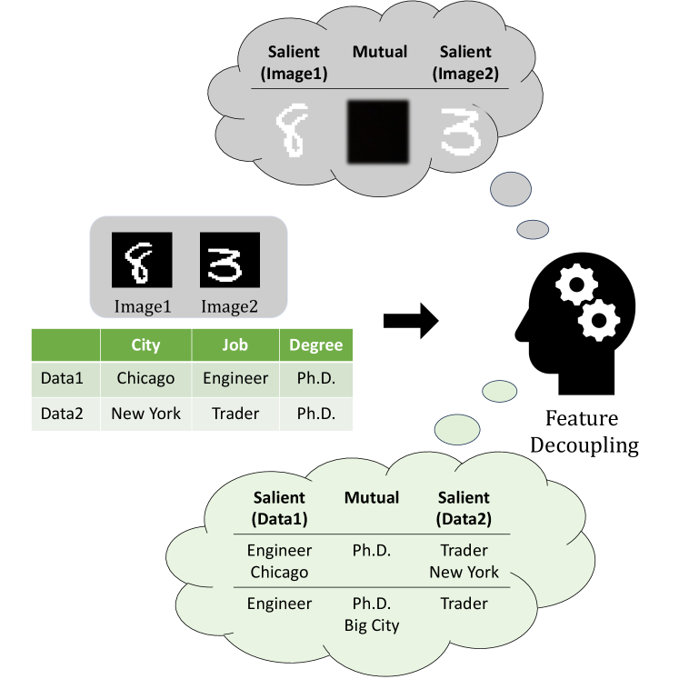
When comparing data samples, mutual features consist of information that highlights common characteristics, while salient features emphasize the distinctive attributes to differentiate one sample from the others. For image data, the intensity of the background pixels forms the mutual features shared across images while the relative positions of bright and dark pixels form the salient features, which are likely to vary significantly across images with different shapes or objects. As illustrated in Figure 1, in MNIST [109], decoupling digits from the background is relatively straightforward, using digits as the salient features for classification. However, the differentiation for tabular data tends to be less distinct. For example, feature like City can be considered salient when the data points “Chicago” and “New York” have different word counts. Nonetheless, when considering the size of city semantically, feature City could share mutual information. Therefore, it becomes more complicated to set the decision boundary for classification.
To tackle these challenges, our central insight revolves around empowering representation models to explicitly distinguish mutual and salient information within the feature space, which we define as the decoupling process. Instead of solely relying on the original data space, We firmly believe that manipulating the feature space could lead to less noise and obtain more representativeness, adapting the success of representation learning from other domains to tabular data.
In this paper, we introduce SwitchTab, an elegant and effective generative pre-training framework for tabular data representation learning. The core of SwitchTab is an asymmetric encoder-decoder structure, augmented with custom projectors that facilitate information decoupling. The process begins with encoding each data sample into a general embedding, which is further projected into salient and mutual embeddings. What sets SwitchTab apart is the deliberate swapping of salient and mutual embeddings among different data samples during decoding. This innovative approach not only allows the model to acquire more structured embeddings from encoder but also explicitly extracts and represents the salient and mutual information. Another advantage of SwitchTab is its versatility, to be trained effectively in both self-supervised manners. This adaptability ensures that SwitchTab performs well in diverse training scenarios, regardless of the availability of labeled data.
Our contributions can be summarized as follows:
-
We propose SwitchTab, a novel self-supervised learning framework to decouple salient and mutual embeddings across data samples. To the best of our knowledge, this is the first attempt to explore and explicitly extract separable and organized embeddings for tabular data.
-
By fine-tuning the pre-trained encoder from SwitchTab, we demonstrate that our method achieves competitive results across extensive datasets and benchmarks.
-
The extracted salient embeddings can be used as plug-and-play features to enhance the performance of various traditional prediction models, e.g., XGBoost.
-
We visualize the structured embeddings learned from SwitchTab and highlight the distinction between mutual and salient information, enhancing the explainability of the proposed framework.
Related Work
Models for Tabular Data Learning and Prediction
Traditional Models.
For tabular data classification and regression tasks, various machine learning methods have been developed. For linear relationships modeling, Logistic Regression (LR) [104, 120] and Generalized Linear Models (GLM) [47, 19] are top choices. Tree-based models include Decision Trees (DT) [14] and various ensemble methods based on DT such as XGBoost [24], Random Forest [13], CatBoost [81] and LightGBM [56], which are widely adopted in industry for modeling complex non-linear relationships, improving interpretability and handling various feature types like null values or categorical features.
Deep Learning Models.
Recent research trends aim to adopt deep learning models to tabular data domain. Various neural architectures have been introduced to improve performance on tabular data. There are several major categories [11, 41], including 1) supervised methods with neural networks (e.g., ResNet [50], SNN [61], AutoInt [90], DCN V2 [100]); 2) hybrid methods to integrate decision trees with neural networks for end-to-end training (e.g., NODE [79], GrowNet [5], TabNN [58], DeepGBM [57]); 3) transformer-based methods to learn from attentions across features and data samples (e.g., TabNet [3], TabTransformer [53], FT-Transformer [41]); and 4) representation learning methods, which have emerging focuses and align with the scope of our proposed work, to realize effective information extraction through self- and semi-supervised learning (e.g., VIME [116], SCARF [6], SAINT [88]) and Recontab[23]. In addition, indirect tabular learning would transfer tabular data into graph [78, 77, 110] and define graph-related tasks for representation learning, such as TabGNN [44].
Self-supervised Representation Learning
Deep representation learning methods have been introduced in the computer vision and remote sensing domains, utilizing self-supervised learning methods [63, 37, 65, 105, 69, 106]. These methods can be divided into two branches. The first branch mainly focuses on a contrastive learning framework with various data augmentation schemes such as artificial augmentations, Fourier transform, or temporal variances[72, 107, 111, 112, 114]. More specifically, models rely on momentum-update strategies [49, 107, 26, 106, 16], large batch sizes [25], stop-gradient operations [27], or training an online network to predict the output of the target network [42]. These ideas have also been applied to the tabular data domain. One representative work in this area is SCARF [6], which adopts the idea of SimCLR [25] to pre-train the encoder using feature corruption as the data augmentation method. Another work is SAINT [88], which also stems from a contrastive learning framework and computes column-wise and row-wise attentions. The second branch is based on generative models such as autoencoders [60]. Specifically, Masked Autoencoder (MAE) [48] has an asymmetric encoder-decoder architecture for learning embeddings from images. This framework is also capable of capturing spatiotemporal information [38] and can be extended to 3D space [55] and multiple scales [85]. The similar masking strategy is widely used in NLP [32] as well as tabular data [3, 53, 115]. A work similar to MAE in the domain of tabular data is VIME [116]. VIME corrupts and encodes each sample in feature space using two estimators. After each estimator, the features are assigned with decoders to reconstruct a binary mask and the original uncorrupted samples, respectively. The key difference between VIME and our work is that we leverage the asymmetric encoder-decoder architecture in pre-training [23] and introduce a switching mechanism, which strongly encourages the encoder to generate more structured and representative embeddings.
Feature Decoupling
In the areas of feature extraction [87, 83, 123] and latent representation learning [8], autoencoder-based models [60, 2] have been widely used for , with strong capabilities to learning useful representations for real-world tasks with little or no supervision. Previous work has been focusing on learning a decoupled representation [51, 59, 12, 119] where each dimension can capture the change of one semantically meaningful factor of variation while being relatively invariant to changes in other factors. Recent work also explored capturing the dependencies and relationships across different factors of variation to enhance the latent representations [89, 93]. Taking one step further, the work of contrastive variational autoencoder (cVAE) by [1], which adapted the contrastive analysis principles, has explicitly categorized latent features by salient and mutual information and enhanced the salient features. The swapping autoencoder by [76] explicitly decouple the image into structure and texture embeddings, which are swapped for image generation. Some recent work for tabular data representation learning has also shown the benefits of quantifying the between-sample relationships. Relational Autoencoder (RAE) [70] considered both the data features and relationships to generate more robust features with lower reconstruction loss and better performance in downstream tasks. [64, 88] shared a similar idea to consider self-attention between data samples. We extend the idea of cVAE and swapping autoencoder to the tabular data domain with the argument that the two data samples share mutual and salient information through latent between-sample relationships. Salient information is crucial for downstream tasks involving decision boundaries, while mutual information remains necessary for data reconstruction. To the best of our knowledge, we are the first to model tabular data with explicit and expressive feature decoupling architecture to enhance the representation learning performance. Meanwhile, feature decoupling could enhance the explainability of the model. Existing work has explored different perspectives such as SHAP value [54], concepts [118], and counterfactual explanations [30, 28, 29], etc. However, explicit learning of salient and mutual information from model structure is yet to be explored.
Method
In this section, we present SwitchTab, our comprehensive approach for tabular data representation learning and feature decoupling. First, we outline the process of feature corruption. Then, in the second sub-section, we delve into the intricacies of self-supervised learning, including data encoding, feature decoupling, and data reconstruction. The third sub-section elucidates our pre-training learning method with labels. Finally, we illustrate how to utilize the pre-trained encoders and embeddings to improve downstream tasks.
Feature Corruption
Generative-based representation learning relies on data augmentations to learn robust embeddings for downstream tasks. Among different methods, feature corruption [116, 6] is one of the most promising approaches. In this paper, we also take advantage of this method to improve the model performance. For one tabular data from original dataset , we define its -th feature as , i.e., , where is the dimension of features and is the index of samples. For each sample, we randomly select features among features and replace them with corrupted feature . Concretely, , where is the uniform distribution over .
Self-supervised Learning
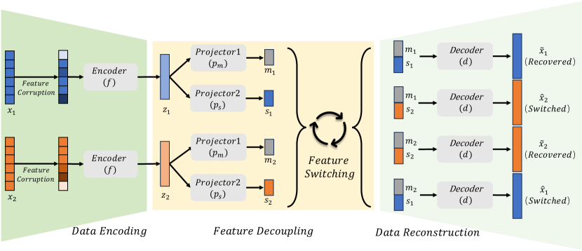
Self-supervised learning of SwitchTab aims to learn informative representations from unlabeled data (Algorithm 1), which is described in Figure 2. For each of the two data samples, and , we apply feature corruption to obtain corrupted data. We encode them using an encoder, , resulting in two feature vectors, and . Importantly, we decouple these two feature vectors using two types of projectors, and , which extract switchable mutual information among the data samples and salient information that is unique to each individual data sample, respectively. Through this decoupling process, we obtain the salient feature vectors, and , and the mutual feature vectors, and , for and , respectively.
Notably, the mutual features should be shared and switchable between two samples. In other words, the concatenated feature vector of should exhibit no discernible difference compared to . Consequently, it is expected that not only should the decoded data (recovered) from be highly similar to , but also the decoded data (switched) from the concatenated feature vector of should demonstrate a comparable level of similarity. Likewise, we anticipate both (recovered) and (switched) to resemble as much. Therefore, we define the loss function as reconstruction loss by:
| (1) |
Pre-training with Labels
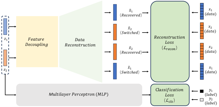
We further improve the pre-training process by taking advantage of labeled data, as shown in Figure 3. With labels introduced, we pose additional constraints to the encoded embeddings and for label prediction and compute the prediction loss (illustrated by classification loss through the context). To be specific, and are fed to the same multi-layer perceptron (MLP) that maps from the embedding space to the label space. During the optimization stage, we combine the prediction loss with above to update the parameters in the framework. Formally, we define the loss function for two samples and as follow:
| (2) |
where is used to balance the classification loss and reconstruction loss and set to 1 as default. To illustrate, the cross-entropy loss for classification task is defined as:
| (3) |
where and are predicted labels, i.e., and . For regression tasks, rooted mean squared error (RMSE) will replace the cross-entropy loss.
| Dataset size | 48842 | 65196 | 83733 | 98050 | 108000 | 500000 | 518012 | 20640 | 515345 | 709877 | 1200192 |
| Feature size | 14 | 27 | 54 | 28 | 128 | 2000 | 54 | 8 | 90 | 699 | 136 |
| Method/Dataset | AD | HE | JA | HI | AL | EP | CO | CA | YE | YA | MI |
| TabNet | 0.850 | 0.378 | 0.723 | 0.719 | 0.954 | 0.8896 | 0.957 | 0.510 | 8.909 | 0.823 | 0.751 |
| SNN | 0.854 | 0.373 | 0.719 | 0.722 | 0.954 | 0.8975 | 0.961 | 0.493 | 8.895 | 0.761 | 0.751 |
| AutoInt | 0.859 | 0.372 | 0.721 | 0.725 | 0.945 | 0.8949 | 0.934 | 0.474 | 8.882 | 0.768 | 0.750 |
| MLP | 0.852 | 0.383 | 0.723 | 0.723 | 0.954 | 0.8977 | 0.962 | 0.499 | 8.853 | 0.757 | 0.747 |
| DCN2 | 0.853 | 0.385 | 0.723 | 0.723 | 0.955 | 0.8977 | 0.965 | 0.484 | 8.890 | 0.757 | 0.749 |
| NODE | 0.858 | 0.359 | 0.726 | 0.726 | 0.918 | 0.8958 | 0.985 | 0.464 | 8.784 | 0.753 | 0.745 |
| ResNet | 0.854 | 0.396 | 0.727 | 0.727 | 0.963 | 0.8969 | 0.964 | 0.486 | 8.846 | 0.757 | 0.748 |
| FT-Transormer | 0.859 | 0.391 | 0.729 | 0.729 | 0.960 | 0.8982 | 0.970 | 0.459 | 8.855 | 0.756 | 0.746 |
| XGBoost | 0.874 | 0.377 | 0.724 | 0.728 | 0.924 | 0.8799 | 0.964 | 0.431 | 8.819 | 0.732 | 0.742 |
| CatBoost | 0.873 | 0.388 | 0.727 | 0.729 | 0.948 | 0.8893 | 0.950 | 0.423 | 8.837 | 0.740 | 0.743 |
| SwitchTab (Self-Sup.) | 0.867 | 0.387 | 0.726 | 0.724 | 0.942 | 0.8928 | 0.971 | 0.452 | 8.857 | 0.755 | 0.751 |
| SwitchTab | 0.881 | 0.389 | 0.731 | 0.733 | 0.951 | 0.8987 | 0.989 | 0.442 | 8.822 | 0.744 | 0.742 |
Downstream Fine-tuning
In line with the established paradigm of representation learning [49, 26, 25, 6], we perform the end-to-end fine-tuning of the pre-trained encoder from SwitchTab using the complete set of labeled data. Specifically, we incorporate the encoder with an additional linear layer, unlocking all its parameters and adapting them for the downstream supervised tasks.
Another avenue to leverage the advantages of our framework lies in harnessing the salient feature vector as a plug-and-play embedding. By concatenating with its original feature vector , we construct enriched data sample vector denoted as . This method effectively highlights the distinct characteristics within the data which facilitates the establishment of a clear decision boundary. As a result, we anticipate noticeable enhancements in classification tasks when utilizing as the input for a traditional model like XGBoost.
Experiments and Results
In this section, we present the results of our comprehensive experiments conducted on various datasets to demonstrate the effectiveness of SwitchTab. The section is divided into two parts. In the first part, we provide preliminary information about the experiments, including the datasets, data preprocessing, model architectures, and training details, aiming to ensure transparency and reproducibility.
In the second part, we evaluate the performance of our proposed method from two distinct perspectives. First, we compare SwitchTab against mainstream deep learning and traditional models using standard benchmarks from [41] and additional datasets to establish a more comprehensive performance assessment of SwitchTab. Secondly, we showcase the versatility of SwitchTab by demonstrating the utilization of salient features as plug-and-play embeddings across various traditional models, including XGBoost, Random Forest, and LightGBM. The plug-and-play strategy allows us to enhance the traditional models performance effortlessly and without additional complexity.
| Dataset size | 45211 | 7043 | 452 | 200 | 12330 | 58310 | 518012 | ||||||||||||||
| Feature size | 16 | 20 | 226 | 783 | 17 | 147 | 54 | ||||||||||||||
| Dataset | BK | BC | AT | AR | SH | VO | MN | ||||||||||||||
| Raw Feature () | ✓ | ✓ | ✓ | ✓ | ✓ | ✓ | ✓ | ✓ | ✓ | ✓ | ✓ | ✓ | ✓ | ✓ | |||||||
| Salient Feature () | ✓ | ✓ | ✓ | ✓ | ✓ | ✓ | ✓ | ✓ | ✓ | ✓ | ✓ | ✓ | ✓ | ✓ | |||||||
| Logistic Reg. | 0.907 | 0.910 | 0.918 | 0.892 | 0.894 | 0.902 | 0.862 | 0.862 | 0.869 | 0.916 | 0.915 | 0.922 | 0.870 | 0.871 | 0.882 | 0.539 | 0.545 | 0.551 | 0.899 | 0.907 | 0.921 |
| Random Forest | 0.891 | 0.895 | 0.902 | 0.879 | 0.880 | 0.899 | 0.850 | 0.853 | 0.885 | 0.809 | 0.810 | 0.846 | 0.929 | 0.931 | 0.933 | 0.663 | 0.669 | 0.672 | 0.938 | 0.940 | 0.945 |
| XGboost | 0.929 | 0.929 | 0.938 | 0.906 | 0.907 | 0.912 | 0.870 | 0.872 | 0.904 | 0.824 | 0.828 | 0.843 | 0.925 | 0.924 | 0.931 | 0.690 | 0.691 | 0.693 | 0.958 | 0.961 | 0.964 |
| LightGBM | 0.939 | 0.939 | 0.942 | 0.910 | 0.910 | 0.915 | 0.887 | 0.889 | 0.903 | 0.821 | 0.826 | 0.831 | 0.932 | 0.933 | 0.944 | 0.679 | 0.682 | 0.686 | 0.952 | 0.955 | 0.963 |
| CatBoost | 0.925 | 0.928 | 0.937 | 0.912 | 0.910 | 0.919 | 0.879 | 0.880 | 0.899 | 0.825 | 0.828 | 0.877 | 0.931 | 0.934 | 0.942 | 0.664 | 0.671 | 0.682 | 0.956 | 0.958 | 0.968 |
| MLP | 0.915 | 0.917 | 0.923 | 0.892 | 0.895 | 0.902 | 0.902 | 0.905 | 0.912 | 0.903 | 0.904 | 0.908 | 0.887 | 0.891 | 0.910 | 0.631 | 0.633 | 0.642 | 0.939 | 0.941 | 0.948 |
| VIME | 0.766 | - | - | 0.510 | - | - | 0.653 | - | - | 0.610 | - | - | 0.744 | - | - | 0.623 | - | - | 0.958 | - | - |
| TabNet | 0.918 | - | - | 0.796 | - | - | 0.521 | - | - | 0.541 | - | - | 0.914 | - | - | 0.568 | - | - | 0.968 | - | - |
| TabTransformer | 0.913 | - | - | 0.817 | - | - | 0.700 | - | - | 0.868 | - | - | 0.927 | - | - | 0.580 | - | - | 0.887 | - | - |
| SAINT | 0.933 | - | - | 0.847 | - | - | 0.941 | - | - | 0.910 | - | - | 0.931 | - | - | 0.701 | - | - | 0.977 | - | - |
| ReConTab | 0.929 | - | - | 0.913 | - | - | 0.907 | - | - | 0.918 | - | - | 0.931 | - | - | 0.680 | - | - | 0.968 | - | - |
| SwitchTab(Self-Sup.) | 0.917 | - | - | 0.903 | - | - | 0.900 | - | - | 0.904 | - | - | 0.931 | - | - | 0.629 | - | - | 0.969 | - | - |
| SwitchTab | 0.942 | - | - | 0.923 | - | - | 0.928 | - | - | 0.922 | - | - | 0.958 | - | - | 0.708 | - | - | 0.982 | - | - |
| indicates the experiments are not applicable for the corresponding methods to demonstrate the benefits of plug-and-play embeddings. | |||||||||||||||||||||
Preliminaries for Experiments
Datasets.
We first evaluate the performance of SwitchTab on a standard benchmark from [41]. Concretely, the datasets include: California Housing (CA) [75], Adult (AD) [62], Helena (HE) [46], Jannis (JA) [46], Higgs (HI) [7], ALOI (AL) [40], Epsilon (EP) [117], Year (YE) [9], Covertype (CO) [10], Yahoo (YA) [15], Microsoft (MI) [84].
Preprocessing of Datasets.
We represent categorical features using a backward difference encoder [80]. Regarding missing data, we discard any features that are missing for all samples. For the remaining missing values, we employ imputation strategies based on the feature type. Numerical features are imputed using the mean value, while categorical features are filled with the most frequent category found within the dataset. Furthermore, we ensure uniformity by scaling the dataset using a Min-Max scaler. When dealing with image-based data, we flatten them into vectors, thus treating them as tabular data, following the approach established in prior works [116, 88].
Model Architectures.
For feature corruption, we uniformly sample a subset of features for each sample to generate a corrupted view at a fixed corruption ratio of 0.3. For the encoder , we employ a three-layer transformer with two heads. The input and output sizes of the encoder are always aligned with the feature size of the input. Both projectors and consist of one linear layer, followed by a sigmoid activation function. Additionally, the decoder remains a one-layer network with a sigmoid activation function. During the pre-training stage with labels, we introduce an additional one-layer network for prediction. In the downstream fine-tuning stage, we append a linear layer after the encoder to accommodate classification or regression tasks.
Training Details.
Importantly, we maintain consistent settings throughout the evaluation of SwitchTab. Although further gains might be attainable with further exploration of hyperparameters, we intentionally refrain from doing so to ensure the proposed approach can be easily generalized across diverse datasets and domains. For all the pre-training, we train all models for 1000 epochs with the default batch size of 128. We use the RMSprop optimizer [52] with an initial learning rate set as 0.0003. During the fine-tuning stage, we set the maximum epochs as 200. Adam optimizer with a learning rate of 0.001 is used.
| Dataset | BK | BC | AT | AR | SH | VO | MN |
| SwitchTab (No Switching) | 0.918 | 0.909 | 0.902 | 0.896 | 0.912 | 0.689 | 0.968 |
| SwitchTab | 0.942 | 0.923 | 0.928 | 0.922 | 0.958 | 0.708 | 0.982 |
Results on Previous Benchmarks
We conduct a comprehensive performance comparison of SwitchTab with different methods across 11 datasets from previous benchmarks, as shown in Table 1. To ensure a fair and direct comparison, we report the accuracy of the classification tasks, following the metrics employed in previous studies. It is worth noting that we meticulously fine-tuned the results in accordance with the established paradigm [63]. Upon analyzing the results, we find that SwitchTab consistently achieves optimal or near-optimal performance in most of the classification tasks. These outcomes underscore the effectiveness and superiority of SwitchTab in representation learning for classification scenarios. However, in regression tasks, we observe that traditional methods like XGBoost or CatBoost still dominate and achieve the best results. Nonetheless, SwitchTab remains highly competitive and outperforms various deep learning approaches in these regression scenarios. We report the averaged results over 10 random seeds.
Results on Additional Public Datasets
Beyond the previous benchmarks, we continue the performance comparisons on additional public datasets and summarize the results in Table 2. The results encompass evaluations using both traditional models and more recent deep learning techniques. In the majority of cases, SwitchTab showcases remarkable improvements, surpassing all baseline methods and reinforcing its superiority across diverse datasets and scenarios. However, it is essential to acknowledge that on the dataset AT, SwitchTab achieved sub-optimal results when compared to the baselines. This observation aligns with previous research conclusions that the tabular domain poses unique challenges where no single method universally dominates [41]. Nevertheless, this outcome merits further investigation to discern the specific factors contributing to this variation in performance.
Plug-and-Play Embeddings
As mentioned earlier, SwitchTab excels in effectively extracting salient features which could significantly influence the decision boundaries for classification tasks. In the plug-and-play setting, our experiment results demonstrate that these salient features have immense value when integrated with original data as additional features. Notably, the performance of all traditional methods can be boosted, improving the evaluation metrics (e.g., AUC) from to (in absolute difference) across various datasets, as illustrated in the dark gray columns Table 2. Meanwhile, we also report results when using only the salient features as input. While the improvement is relatively marginal, it aligns with our expectations. The absence of mutual information in this scenario leads to a less substantial performance boost.
Visualization and Discussions
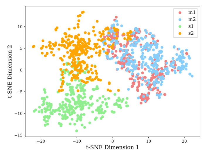
In this section, we visualize the features learned by SwitchTab using the BK dataset, which is designed for binary classification tasks. After pre-training, we feed the first batch with data from one class and the second batch with data from the other class, and then visualize the corresponding feature vectors. As shown in Figure 4, the embeddings and from SwitchTab, although extracted from two different classes, heavily overlap with each other. This substantiates the fact that the mutual information is switchable. However, the salient feature and the salient feature are distinctly separated, playing a dominant role in capturing the unique properties of each class and decisively contributing to the classification boundaries.
Ablation Studies
In this section, we investigate essential modules of SwitchTab, including the importance of the switching process, the feature corruption rate and the computation cost. We use all of the datasets in Table 2, with all the same data preprocessing and optimization strategies.
Contribution of Switching Process.
To demonstrate that the superior performance of the proposed model directly results from the critical switching process, we report the results with and without reconstructing the concatenated features from switched pairs, i.e., and , keeping the feature corruption ratio at 0.3 for all experiments. Notably, without the switching mechanism, the framework deteriorates to a simpler auto-encoder structure and results in obvious drop in evaluation metrics (e.g., AUC) in Table 3.
Feature Corruption Ratio.
We also explore the optimal feature corruption ratio in Table 4. Through extensive analysis, we find that the optimal corruption ratio is approximately 0.3. Therefore, we adopt this value as the default for all previously reported experiments. However, it is essential to emphasize that this selected ratio may not be consistently optimal for each dataset. We also observe that datasets with higher feature dimensions, such as AR or VO, tend to benefit from larger corruption ratios, since they are more likely to have redundant features. This observation is aligned with previous conclusions on tabular data from [43]. Conversely, for datasets with low-dimensional features such as BC, smaller corruption ratios could also yield superior results in our experiments.
| Ratio | 0.0 | 0.1 | 0.2 | 0.3 | 0.4 | 0.5 | 0.6 |
| BK | 0.927 | 0.938 | 0.940 | 0.942 | 0.932 | 0.903 | 0.898 |
| BC | 0.911 | 0.920 | 0.923 | 0.923 | 0.917 | 0.910 | 0.902 |
| AT | 0.916 | 0.922 | 0.925 | 0.928 | 0.927 | 0.920 | 0.913 |
| AR | 0.913 | 0.915 | 0.918 | 0.922 | 0.925 | 0.920 | 0.914 |
| SH | 0.948 | 0.956 | 0.956 | 0.958 | 0.947 | 0.934 | 0.922 |
| VO | 0.683 | 0.694 | 0.699 | 0.708 | 0.709 | 0.700 | 0.692 |
| MN | 0.969 | 0.971 | 0.977 | 0.982 | 0.978 | 0.966 | 0.957 |
Conclusion
Motivated by the profound success of representation learning in computation vision and natural language processing domains, we want to extend this success to tabular data domain. Differentiating from other related studies to address this issue from a contrastive learning perspective, we introduce SwitchTab, a novel pre-training framework for representation learning from the perspective of generative models. The learned embeddings from SwitchTab could not only achieve superior performance on downstream tasks but also represent a distinguishable salient feature space that can enhance a broader range of traditional methods as plug-and-play embeddings. We firmly believe that this work constitutes a critical step towards achieving more representative, explainable, and structured representations for tabular data.
References
- Abid and Zou [2019] Abid, A.; and Zou, J. Y. 2019. Contrastive Variational Autoencoder Enhances Salient Features. ArXiv, abs/1902.04601.
- Abukmeil et al. [2021] Abukmeil, M.; Ferrari, S.; Genovese, A.; Piuri, V.; and Scotti, F. 2021. A survey of unsupervised generative models for exploratory data analysis and representation learning. Acm computing surveys (csur), 54(5): 1–40.
- Arik and Pfister [2021] Arik, S. Ö.; and Pfister, T. 2021. Tabnet: Attentive interpretable tabular learning. In Proceedings of the AAAI conference on artificial intelligence, volume 35, 6679–6687.
- Asuncion and Newman [2007] Asuncion, A.; and Newman, D. 2007. UCI machine learning repository.
- Badirli et al. [2020] Badirli, S.; Liu, X.; Xing, Z.; Bhowmik, A.; Doan, K.; and Keerthi, S. S. 2020. Gradient boosting neural networks: Grownet. arXiv preprint arXiv:2002.07971.
- Bahri et al. [2021] Bahri, D.; Jiang, H.; Tay, Y.; and Metzler, D. 2021. Scarf: Self-supervised contrastive learning using random feature corruption. arXiv preprint arXiv:2106.15147.
- Baldi, Sadowski, and Whiteson [2014] Baldi, P.; Sadowski, P.; and Whiteson, D. 2014. Searching for exotic particles in high-energy physics with deep learning. Nature communications, 5(1): 4308.
- Bengio, Courville, and Vincent [2013] Bengio, Y.; Courville, A.; and Vincent, P. 2013. Representation learning: A review and new perspectives. IEEE transactions on pattern analysis and machine intelligence, 35(8): 1798–1828.
- Bertin-Mahieux et al. [2011] Bertin-Mahieux, T.; Ellis, D. P.; Whitman, B.; and Lamere, P. 2011. The million song dataset. academiccommons.columbia.edu.
- Blackard and Dean [1999] Blackard, J. A.; and Dean, D. J. 1999. Comparative accuracies of artificial neural networks and discriminant analysis in predicting forest cover types from cartographic variables. Computers and electronics in agriculture, 24(3): 131–151.
- Borisov et al. [2022] Borisov, V.; Leemann, T.; Seßler, K.; Haug, J.; Pawelczyk, M.; and Kasneci, G. 2022. Deep neural networks and tabular data: A survey. IEEE Transactions on Neural Networks and Learning Systems.
- Bousmalis et al. [2016] Bousmalis, K.; Trigeorgis, G.; Silberman, N.; Krishnan, D.; and Erhan, D. 2016. Domain separation networks. Advances in neural information processing systems, 29.
- Breiman [2001] Breiman, L. 2001. Random forests. Machine learning, 45: 5–32.
- Breiman [2017] Breiman, L. 2017. Classification and regression trees. Routledge.
- Chapelle and Chang [2011] Chapelle, O.; and Chang, Y. 2011. Yahoo! learning to rank challenge overview. In Proceedings of the learning to rank challenge, 1–24. PMLR.
- Che et al. [2023] Che, C.; Lin, Q.; Zhao, X.; Huang, J.; and Yu, L. 2023. Enhancing Multimodal Understanding with CLIP-Based Image-to-Text Transformation. In Proceedings of the 2023 6th International Conference on Big Data Technologies, 414–418.
- Chen [2020] Chen, S. 2020. Some Recent Advances in Design of Bayesian Binomial Reliability Demonstration Tests. USF Tampa Graduate Theses and Dissertations.
- Chen et al. [2017] Chen, S.; Kearns, W. D.; Fozard, J. L.; and Li, M. 2017. Personalized fall risk assessment for long-term care services improvement. In 2017 Annual Reliability and Maintainability Symposium (RAMS), 1–7. IEEE.
- Chen et al. [2019] Chen, S.; Kong, N.; Sun, X.; Meng, H.; and Li, M. 2019. Claims data-driven modeling of hospital time-to-readmission risk with latent heterogeneity. Health care management science, 22: 156–179.
- Chen, Lu, and Li [2017] Chen, S.; Lu, L.; and Li, M. 2017. Multi-state reliability demonstration tests. Quality Engineering, 29(3): 431–445.
- Chen et al. [2018] Chen, S.; Lu, L.; Xiang, Y.; Lu, Q.; and Li, M. 2018. A data heterogeneity modeling and quantification approach for field pre-assessment of chloride-induced corrosion in aging infrastructures. Reliability Engineering & System Safety, 171: 123–135.
- Chen et al. [2020a] Chen, S.; Lu, L.; Zhang, Q.; and Li, M. 2020a. Optimal binomial reliability demonstration tests design under acceptance decision uncertainty. Quality Engineering, 32(3): 492–508.
- Chen et al. [2023] Chen, S.; Wu, J.; Hovakimyan, N.; and Yao, H. 2023. ReConTab: Regularized Contrastive Representation Learning for Tabular Data. arXiv preprint arXiv:2310.18541.
- Chen and Guestrin [2016] Chen, T.; and Guestrin, C. 2016. Xgboost: A scalable tree boosting system. In Proceedings of the 22nd acm sigkdd international conference on knowledge discovery and data mining, 785–794.
- Chen et al. [2020b] Chen, T.; Kornblith, S.; Norouzi, M.; and Hinton, G. 2020b. A simple framework for contrastive learning of visual representations. In International conference on machine learning, 1597–1607. PMLR.
- Chen et al. [2020c] Chen, X.; Fan, H.; Girshick, R.; and He, K. 2020c. Improved baselines with momentum contrastive learning. arXiv preprint arXiv:2003.04297.
- Chen and He [2021] Chen, X.; and He, K. 2021. Exploring simple siamese representation learning. In Proceedings of the IEEE/CVF Conference on Computer Vision and Pattern Recognition, 15750–15758.
- Chen et al. [2022a] Chen, Z.; Silvestri, F.; Tolomei, G.; Wang, J.; Zhu, H.; and Ahn, H. 2022a. Explain the Explainer: Interpreting Model-Agnostic Counterfactual Explanations of a Deep Reinforcement Learning Agent. IEEE Transactions on Artificial Intelligence.
- Chen et al. [2022b] Chen, Z.; Silvestri, F.; Wang, J.; Zhang, Y.; Huang, Z.; Ahn, H.; and Tolomei, G. 2022b. Grease: Generate factual and counterfactual explanations for gnn-based recommendations. arXiv preprint arXiv:2208.04222.
- Chen et al. [2022c] Chen, Z.; Silvestri, F.; Wang, J.; Zhu, H.; Ahn, H.; and Tolomei, G. 2022c. Relax: Reinforcement learning agent explainer for arbitrary predictive models. In Proceedings of the 31st ACM International Conference on Information & Knowledge Management, 252–261.
- Covert, Sumbul, and Lee [2019] Covert, I.; Sumbul, U.; and Lee, S.-I. 2019. Deep unsupervised feature selection. ’ ’.
- Devlin et al. [2018] Devlin, J.; Chang, M.-W.; Lee, K.; and Toutanova, K. 2018. Bert: Pre-training of deep bidirectional transformers for language understanding. arXiv preprint arXiv:1810.04805.
- Dong et al. [2021a] Dong, G.; Boukhechba, M.; Shaffer, K. M.; Ritterband, L. M.; Gioeli, D. G.; Reilley, M. J.; Le, T. M.; Kunk, P. R.; Bauer, T. W.; and Chow, P. I. 2021a. Using graph representation learning to predict salivary cortisol levels in pancreatic cancer patients. Journal of Healthcare Informatics Research, 5: 401–419.
- Dong et al. [2022] Dong, G.; Kweon, Y.; Park, B. B.; and Boukhechba, M. 2022. Utility-based route choice behavior modeling using deep sequential models. Journal of big data analytics in transportation, 4(2-3): 119–133.
- Dong et al. [2021b] Dong, G.; Tang, M.; Cai, L.; Barnes, L. E.; and Boukhechba, M. 2021b. Semi-supervised graph instance transformer for mental health inference. In 2021 20th IEEE International Conference on Machine Learning and Applications (ICMLA), 1221–1228. IEEE.
- Dong et al. [2023] Dong, G.; Tang, M.; Wang, Z.; Gao, J.; Guo, S.; Cai, L.; Gutierrez, R.; Campbel, B.; Barnes, L. E.; and Boukhechba, M. 2023. Graph neural networks in IoT: a survey. ACM Transactions on Sensor Networks, 19(2): 1–50.
- Ericsson et al. [2022] Ericsson, L.; Gouk, H.; Loy, C. C.; and Hospedales, T. M. 2022. Self-supervised representation learning: Introduction, advances, and challenges. IEEE Signal Processing Magazine, 39(3): 42–62.
- Feichtenhofer et al. [2022] Feichtenhofer, C.; Li, Y.; He, K.; et al. 2022. Masked autoencoders as spatiotemporal learners. Advances in neural information processing systems, 35: 35946–35958.
- Gao et al. [2023] Gao, L.; Cordova, G.; Danielson, C.; and Fierro, R. 2023. Autonomous Multi-Robot Servicing for Spacecraft Operation Extension. In 2023 IEEE/RSJ International Conference on Intelligent Robots and Systems (IROS), 10729–10735. IEEE.
- Geusebroek, Burghouts, and Smeulders [2005] Geusebroek, J.-M.; Burghouts, G. J.; and Smeulders, A. W. 2005. The Amsterdam library of object images. International Journal of Computer Vision, 61: 103–112.
- Gorishniy et al. [2021] Gorishniy, Y.; Rubachev, I.; Khrulkov, V.; and Babenko, A. 2021. Revisiting deep learning models for tabular data. Advances in Neural Information Processing Systems, 34: 18932–18943.
- Grill et al. [2020] Grill, J.-B.; Strub, F.; Altché, F.; Tallec, C.; Richemond, P.; Buchatskaya, E.; Doersch, C.; Avila Pires, B.; Guo, Z.; Gheshlaghi Azar, M.; et al. 2020. Bootstrap your own latent-a new approach to self-supervised learning. Advances in neural information processing systems, 33: 21271–21284.
- Grinsztajn, Oyallon, and Varoquaux [2022] Grinsztajn, L.; Oyallon, E.; and Varoquaux, G. 2022. Why do tree-based models still outperform deep learning on typical tabular data? Advances in Neural Information Processing Systems, 35: 507–520.
- Guo et al. [2021] Guo, X.; Quan, Y.; Zhao, H.; Yao, Q.; Li, Y.; and Tu, W. 2021. TabGNN: Multiplex graph neural network for tabular data prediction. arXiv preprint arXiv:2108.09127.
- Guyon et al. [2019a] Guyon, I.; Sun-Hosoya, L.; Boullé, M.; Escalante, H. J.; Escalera, S.; Liu, Z.; Jajetic, D.; Ray, B.; Saeed, M.; Sebag, M.; Statnikov, A.; Tu, W.; and Viegas, E. 2019a. Analysis of the AutoML Challenge series 2015-2018. In AutoML, Springer series on Challenges in Machine Learning.
- Guyon et al. [2019b] Guyon, I.; Sun-Hosoya, L.; Boullé, M.; Escalante, H. J.; Escalera, S.; Liu, Z.; Jajetic, D.; Ray, B.; Saeed, M.; Sebag, M.; et al. 2019b. Analysis of the AutoML challenge series. Automated Machine Learning, 177.
- Hastie and Pregibon [2017] Hastie, T. J.; and Pregibon, D. 2017. Generalized linear models. In Statistical models in S, 195–247. Routledge.
- He et al. [2022] He, K.; Chen, X.; Xie, S.; Li, Y.; Dollár, P.; and Girshick, R. 2022. Masked autoencoders are scalable vision learners. In Proceedings of the IEEE/CVF conference on computer vision and pattern recognition, 16000–16009.
- He et al. [2020] He, K.; Fan, H.; Wu, Y.; Xie, S.; and Girshick, R. 2020. Momentum contrast for unsupervised visual representation learning. In Proceedings of the IEEE/CVF conference on computer vision and pattern recognition, 9729–9738.
- He et al. [2016] He, K.; Zhang, X.; Ren, S.; and Sun, J. 2016. Deep residual learning for image recognition. In Proceedings of the IEEE conference on computer vision and pattern recognition, 770–778.
- Higgins et al. [2016] Higgins, I.; Matthey, L.; Pal, A.; Burgess, C.; Glorot, X.; Botvinick, M.; Mohamed, S.; and Lerchner, A. 2016. beta-vae: Learning basic visual concepts with a constrained variational framework. In International conference on learning representations.
- Hinton, Srivastava, and Swersky [2012] Hinton, G.; Srivastava, N.; and Swersky, K. 2012. Neural networks for machine learning lecture 6a overview of mini-batch gradient descent. Cited on, 14(8): 2.
- Huang et al. [2020] Huang, X.; Khetan, A.; Cvitkovic, M.; and Karnin, Z. 2020. Tabtransformer: Tabular data modeling using contextual embeddings. arXiv preprint arXiv:2012.06678.
- Jethani et al. [2022] Jethani, N.; Sudarshan, M.; Covert, I.; Lee, S.-I.; and Ranganath, R. 2022. Fastshap: Real-time shapley value estimation. ICLR 2022.
- Jiang et al. [2022] Jiang, J.; Lu, X.; Zhao, L.; Dazeley, R.; and Wang, M. 2022. Masked autoencoders in 3D point cloud representation learning. arXiv preprint arXiv:2207.01545.
- Ke et al. [2017] Ke, G.; Meng, Q.; Finley, T.; Wang, T.; Chen, W.; Ma, W.; Ye, Q.; and Liu, T.-Y. 2017. Lightgbm: A highly efficient gradient boosting decision tree. Advances in neural information processing systems, 30.
- Ke et al. [2019] Ke, G.; Xu, Z.; Zhang, J.; Bian, J.; and Liu, T.-Y. 2019. DeepGBM: A deep learning framework distilled by GBDT for online prediction tasks. In Proceedings of the 25th ACM SIGKDD International Conference on Knowledge Discovery & Data Mining, 384–394.
- Ke et al. [2018] Ke, G.; Zhang, J.; Xu, Z.; Bian, J.; and Liu, T.-Y. 2018. TabNN: A universal neural network solution for tabular data.
- Kim and Mnih [2018] Kim, H.; and Mnih, A. 2018. Disentangling by factorising. In International Conference on Machine Learning, 2649–2658. PMLR.
- Kingma and Welling [2013] Kingma, D. P.; and Welling, M. 2013. Auto-encoding variational bayes. arXiv preprint arXiv:1312.6114.
- Klambauer et al. [2017] Klambauer, G.; Unterthiner, T.; Mayr, A.; and Hochreiter, S. 2017. Self-normalizing neural networks. Advances in neural information processing systems, 30.
- Kohavi et al. [1996] Kohavi, R.; et al. 1996. Scaling up the accuracy of naive-bayes classifiers: A decision-tree hybrid. In Kdd, volume 96, 202–207.
- Kolesnikov, Zhai, and Beyer [2019] Kolesnikov, A.; Zhai, X.; and Beyer, L. 2019. Revisiting self-supervised visual representation learning. In Proceedings of the IEEE/CVF conference on computer vision and pattern recognition, 1920–1929.
- Kossen et al. [2021] Kossen, J.; Band, N.; Lyle, C.; Gomez, A. N.; Rainforth, T.; and Gal, Y. 2021. Self-attention between datapoints: Going beyond individual input-output pairs in deep learning. Advances in Neural Information Processing Systems, 34: 28742–28756.
- Li, Guo, and Schuurmans [2015] Li, X.; Guo, Y.; and Schuurmans, D. 2015. Semi-supervised zero-shot classification with label representation learning. In Proceedings of the IEEE international conference on computer vision, 4211–4219.
- Li et al. [2023] Li, Z.; Chen, Z.; Li, Y.; and Xu, C. 2023. Context-aware trajectory prediction for autonomous driving in heterogeneous environments. Computer-Aided Civil and Infrastructure Engineering.
- Liakos et al. [2018] Liakos, K. G.; Busato, P.; Moshou, D.; Pearson, S.; and Bochtis, D. 2018. Machine learning in agriculture: A review. Sensors, 18(8): 2674.
- Liu, Ting, and Zhou [2008] Liu, F. T.; Ting, K. M.; and Zhou, Z.-H. 2008. Isolation forest. In 2008 eighth ieee international conference on data mining, 413–422. IEEE.
- Manas et al. [2021] Manas, O.; Lacoste, A.; Giró-i Nieto, X.; Vazquez, D.; and Rodriguez, P. 2021. Seasonal contrast: Unsupervised pre-training from uncurated remote sensing data. In Proceedings of the IEEE/CVF International Conference on Computer Vision, 9414–9423.
- Meng et al. [2017] Meng, Q.; Catchpoole, D.; Skillicom, D.; and Kennedy, P. J. 2017. Relational autoencoder for feature extraction. In 2017 International joint conference on neural networks (IJCNN), 364–371. IEEE.
- Moro, Cortez, and Rita [2014] Moro, S.; Cortez, P.; and Rita, P. 2014. A data-driven approach to predict the success of bank telemarketing. Decision Support Systems, 62: 22–31.
- Nachum and Yang [2021] Nachum, O.; and Yang, M. 2021. Provable representation learning for imitation with contrastive fourier features. Advances in Neural Information Processing Systems, 34: 30100–30112.
- Osorio, Liu, and Ouyang [2022] Osorio, J.; Liu, Y.; and Ouyang, Y. 2022. Executive orders or public fear: What caused transit ridership to drop in Chicago during COVID-19? Transportation Research Part D: Transport and Environment, 105: 103226.
- Ouk, Dada, and Kang [2018] Ouk, J.; Dada, D.; and Kang, K. T. 2018. Telco Customer Churn.
- Pace and Barry [1997] Pace, R. K.; and Barry, R. 1997. Sparse spatial autoregressions. Statistics & Probability Letters, 33(3): 291–297.
- Park et al. [2020] Park, T.; Zhu, J.-Y.; Wang, O.; Lu, J.; Shechtman, E.; Efros, A.; and Zhang, R. 2020. Swapping autoencoder for deep image manipulation. Advances in Neural Information Processing Systems, 33: 7198–7211.
- Peng et al. [2023a] Peng, H.; Ran, R.; Luo, Y.; Zhao, J.; Huang, S.; Thorat, K.; Geng, T.; Wang, C.; Xu, X.; Wen, W.; et al. 2023a. Lingcn: Structural linearized graph convolutional network for homomorphically encrypted inference. arXiv preprint arXiv:2309.14331.
- Peng et al. [2023b] Peng, H.; Xie, X.; Shivdikar, K.; Hasan, M.; Zhao, J.; Huang, S.; Khan, O.; Kaeli, D.; and Ding, C. 2023b. MaxK-GNN: Towards Theoretical Speed Limits for Accelerating Graph Neural Networks Training. arXiv preprint arXiv:2312.08656.
- Popov, Morozov, and Babenko [2019] Popov, S.; Morozov, S.; and Babenko, A. 2019. Neural oblivious decision ensembles for deep learning on tabular data. arXiv preprint arXiv:1909.06312.
- Potdar, Pardawala, and Pai [2017] Potdar, K.; Pardawala, T. S.; and Pai, C. D. 2017. A comparative study of categorical variable encoding techniques for neural network classifiers. International journal of computer applications, 175(4): 7–9.
- Prokhorenkova et al. [2018] Prokhorenkova, L.; Gusev, G.; Vorobev, A.; Dorogush, A. V.; and Gulin, A. 2018. CatBoost: unbiased boosting with categorical features. Advances in neural information processing systems, 31.
- Qayyum et al. [2020] Qayyum, A.; Qadir, J.; Bilal, M.; and Al-Fuqaha, A. 2020. Secure and robust machine learning for healthcare: A survey. IEEE Reviews in Biomedical Engineering, 14: 156–180.
- Qiao et al. [2023] Qiao, Q.; Li, Y.; Zhou, K.; and Li, Q. 2023. Relation-Aware Network with Attention-Based Loss for Few-Shot Knowledge Graph Completion. In Pacific-Asia Conference on Knowledge Discovery and Data Mining, 99–111. Springer.
- Qin and Liu [2013] Qin, T.; and Liu, T.-Y. 2013. Introducing LETOR 4.0 datasets. arXiv preprint arXiv:1306.2597.
- Reed et al. [2022] Reed, C. J.; Gupta, R.; Li, S.; Brockman, S.; Funk, C.; Clipp, B.; Candido, S.; Uyttendaele, M.; and Darrell, T. 2022. Scale-mae: A scale-aware masked autoencoder for multiscale geospatial representation learning. arXiv preprint arXiv:2212.14532.
- Sakar et al. [2019] Sakar, C. O.; Polat, S. O.; Katircioglu, M.; and Kastro, Y. 2019. Real-time prediction of online shoppers’ purchasing intention using multilayer perceptron and LSTM recurrent neural networks. Neural Computing and Applications, 31: 6893–6908.
- Salau and Jain [2019] Salau, A. O.; and Jain, S. 2019. Feature extraction: a survey of the types, techniques, applications. In 2019 international conference on signal processing and communication (ICSC), 158–164. IEEE.
- Somepalli et al. [2021] Somepalli, G.; Goldblum, M.; Schwarzschild, A.; Bruss, C. B.; and Goldstein, T. 2021. Saint: Improved neural networks for tabular data via row attention and contrastive pre-training. arXiv preprint arXiv:2106.01342.
- Sønderby et al. [2016] Sønderby, C. K.; Raiko, T.; Maaløe, L.; Sønderby, S. K.; and Winther, O. 2016. Ladder variational autoencoders. Advances in neural information processing systems, 29.
- Song et al. [2019] Song, W.; Shi, C.; Xiao, Z.; Duan, Z.; Xu, Y.; Zhang, M.; and Tang, J. 2019. Autoint: Automatic feature interaction learning via self-attentive neural networks. In Proceedings of the 28th ACM international conference on information and knowledge management, 1161–1170.
- Tang et al. [2023] Tang, M.; Gao, J.; Dong, G.; Yang, C.; Campbell, B.; Bowman, B.; Zoellner, J. M.; Abdel-Rahman, E.; and Boukhechba, M. 2023. SRDA: Mobile Sensing based Fluid Overload Detection for End Stage Kidney Disease Patients using Sensor Relation Dual Autoencoder. In Conference on Health, Inference, and Learning, 133–146. PMLR.
- Tao et al. [2022] Tao, R.; Zhao, P.; Wu, J.; Martin, N. F.; Harrison, M. T.; Ferreira, C.; Kalantari, Z.; and Hovakimyan, N. 2022. Optimizing crop management with reinforcement learning and imitation learning. arXiv preprint arXiv:2209.09991.
- Tschannen, Bachem, and Lucic [2018] Tschannen, M.; Bachem, O.; and Lucic, M. 2018. Recent advances in autoencoder-based representation learning. arXiv preprint arXiv:1812.05069.
- Wang et al. [2023a] Wang, B.; Lu, L.; Chen, S.; and Li, M. 2023a. Optimal test design for reliability demonstration under multi-stage acceptance uncertainties. Quality Engineering, 0(0): 1–14.
- Wang, Wu, and Kozlowski [2018] Wang, C.; Wu, X.; and Kozlowski, T. 2018. Surrogate-based bayesian calibration of thermal-hydraulics models based on psbt time-dependent benchmark data. In Proc. ANS Best Estimate Plus Uncertainty International Conference, Real Collegio, Lucca, Italy.
- Wang, Wu, and Kozlowski [2019a] Wang, C.; Wu, X.; and Kozlowski, T. 2019a. Gaussian process–based inverse uncertainty quantification for trace physical model parameters using steady-state psbt benchmark. Nuclear Science and Engineering, 193(1-2): 100–114.
- Wang, Wu, and Kozlowski [2019b] Wang, C.; Wu, X.; and Kozlowski, T. 2019b. Inverse uncertainty quantification by hierarchical bayesian inference for trace physical model parameters based on bfbt benchmark. Proceedings of NURETH-2019, Portland, Oregon, USA.
- Wang, Wu, and Kozlowski [2023] Wang, C.; Wu, X.; and Kozlowski, T. 2023. Inverse Uncertainty Quantification by Hierarchical Bayesian Modeling and Application in Nuclear System Thermal-Hydraulics Codes. arXiv preprint arXiv:2305.16622.
- Wang et al. [2023b] Wang, C.; Wu, X.; Xie, Z.; and Kozlowski, T. 2023b. Scalable Inverse Uncertainty Quantification by Hierarchical Bayesian Modeling and Variational Inference. Energies, 16(22): 7664.
- Wang et al. [2021] Wang, R.; Shivanna, R.; Cheng, D.; Jain, S.; Lin, D.; Hong, L.; and Chi, E. 2021. Dcn v2: Improved deep & cross network and practical lessons for web-scale learning to rank systems. In Proceedings of the web conference 2021, 1785–1797.
- Wang, Li, and Sun [2023] Wang, Y.; Li, D.; and Sun, R. 2023. NTK-SAP: Improving neural network pruning by aligning training dynamics. arXiv preprint arXiv:2304.02840.
- Wang et al. [2023c] Wang, Y.; Su, J.; Lu, H.; Xie, C.; Liu, T.; Yuan, J.; Lin, H.; Sun, R.; and Yang, H. 2023c. LEMON: Lossless model expansion. arXiv preprint arXiv:2310.07999.
- Wang et al. [2023d] Wang, Y.; Wu, J.; Hovakimyan, N.; and Sun, R. 2023d. Balanced Training for Sparse GANs. In Thirty-seventh Conference on Neural Information Processing Systems.
- Wright [1995] Wright, R. E. 1995. Logistic regression.
- Wu, Hobbs, and Hovakimyan [2023] Wu, J.; Hobbs, J.; and Hovakimyan, N. 2023. Hallucination improves the performance of unsupervised visual representation learning. In Proceedings of the IEEE/CVF International Conference on Computer Vision, 16132–16143.
- Wu, Hovakimyan, and Hobbs [2023] Wu, J.; Hovakimyan, N.; and Hobbs, J. 2023. Genco: An auxiliary generator from contrastive learning for enhanced few-shot learning in remote sensing. arXiv preprint arXiv:2307.14612.
- Wu et al. [2023] Wu, J.; Pichler, D.; Marley, D.; Wilson, D.; Hovakimyan, N.; and Hobbs, J. 2023. Extended Agriculture-Vision: An Extension of a Large Aerial Image Dataset for Agricultural Pattern Analysis. arXiv preprint arXiv:2303.02460.
- Wu et al. [2022] Wu, J.; Tao, R.; Zhao, P.; Martin, N. F.; and Hovakimyan, N. 2022. Optimizing nitrogen management with deep reinforcement learning and crop simulations. In Proceedings of the IEEE/CVF conference on computer vision and pattern recognition, 1712–1720.
- Xiao, Rasul, and Vollgraf [2017] Xiao, H.; Rasul, K.; and Vollgraf, R. 2017. Fashion-mnist: a novel image dataset for benchmarking machine learning algorithms. arXiv preprint arXiv:1708.07747.
- Xie et al. [2023] Xie, X.; Peng, H.; Hasan, A.; Huang, S.; Zhao, J.; Fang, H.; Zhang, W.; Geng, T.; Khan, O.; and Ding, C. 2023. Accel-gcn: High-performance gpu accelerator design for graph convolution networks. In 2023 IEEE/ACM International Conference on Computer Aided Design (ICCAD), 01–09. IEEE.
- Ye et al. [2023a] Ye, J.; Kang, H.; Wang, H.; Altaleb, S.; Heidari, E.; Asadizanjani, N.; Sorger, V. J.; and Dalir, H. 2023a. Multiplexed OAM beams classification via Fourier optical convolutional neural network. In 2023 IEEE Photonics Conference (IPC), 1–2. IEEE.
- Ye et al. [2023b] Ye, J.; Kang, H.; Wang, H.; Altaleb, S.; Heidari, E.; Asadizanjani, N.; Sorger, V. J.; and Dalir, H. 2023b. OAM beams multiplexing and classification under atmospheric turbulence via Fourier convolutional neural network. In Frontiers in Optics, JTu4A–73. Optica Publishing Group.
- Ye et al. [2023c] Ye, J.; Kang, H.; Wang, H.; Shen, C.; Jahannia, B.; Heidari, E.; Asadizanjani, N.; Miri, M.-A.; Sorger, V. J.; and Dalir, H. 2023c. Demultiplexing OAM beams via Fourier optical convolutional neural network. In Laser Beam Shaping XXIII, volume 12667, 16–33. SPIE.
- Ye et al. [2023d] Ye, J.; Solyanik, M.; Hu, Z.; Dalir, H.; Nouri, B. M.; and Sorger, V. J. 2023d. Free-space optical multiplexed orbital angular momentum beam identification system using Fourier optical convolutional layer based on 4f system. In Complex Light and Optical Forces XVII, volume 12436, 70–80. SPIE.
- Yin et al. [2020] Yin, P.; Neubig, G.; Yih, W.-t.; and Riedel, S. 2020. TaBERT: Pretraining for joint understanding of textual and tabular data. arXiv preprint arXiv:2005.08314.
- Yoon et al. [2020] Yoon, J.; Zhang, Y.; Jordon, J.; and van der Schaar, M. 2020. Vime: Extending the success of self-and semi-supervised learning to tabular domain. Advances in Neural Information Processing Systems, 33: 11033–11043.
- Yuan, Ho, and Lin [2011] Yuan, G.-X.; Ho, C.-H.; and Lin, C.-J. 2011. An improved glmnet for l1-regularized logistic regression. In Proceedings of the 17th ACM SIGKDD international conference on Knowledge discovery and data mining, 33–41.
- Zarlenga et al. [2023] Zarlenga, M. E.; Shams, Z.; Nelson, M. E.; Kim, B.; and Jamnik, M. 2023. TabCBM: Concept-based Interpretable Neural Networks for Tabular Data. Transactions on Machine Learning Research.
- Zhang et al. [2020] Zhang, H.; Wang, M.; Liu, Y.; and Yuan, Y. 2020. FDN: Feature decoupling network for head pose estimation. In Proceedings of the AAAI conference on artificial intelligence, volume 34, 12789–12796.
- Zhang and Yang [2020] Zhang, Z.; and Yang, X. 2020. Freeway traffic speed estimation by regression machine-learning techniques using probe vehicle and sensor detector data. Journal of transportation engineering, Part A: Systems, 146(12): 04020138.
- Zhang et al. [2023] Zhang, Z.; Yuan, Y.; Li, M.; Lu, P.; and Yang, X. T. 2023. Empirical study of the effects of physics-guided machine learning on freeway traffic flow modelling: model comparisons using field data. Transportmetrica A: Transport Science, 1–28.
- Zhang, Yuan, and Yang [2020] Zhang, Z.; Yuan, Y.; and Yang, X. 2020. A hybrid machine learning approach for freeway traffic speed estimation. Transportation research record, 2674(10): 68–78.
- Zhou et al. [2023] Zhou, K.; Qiao, Q.; Li, Y.; and Li, Q. 2023. Improving distantly supervised relation extraction by natural language inference. In Proceedings of the AAAI Conference on Artificial Intelligence, volume 37, 14047–14055.
- Zhu et al. [2018] Zhu, L.; Yu, F. R.; Wang, Y.; Ning, B.; and Tang, T. 2018. Big data analytics in intelligent transportation systems: A survey. IEEE Transactions on Intelligent Transportation Systems, 20(1): 383–398.