Symmetry, spin-texture, and tunable quantum geometry in a WTe2 monolayer
Abstract
The spin orientation of electronic wavefunctions in crystals is an internal degree of freedom, typically insensitive to electrical knobs. We argue from a general symmetry analysis and a perspective, that monolayer 1T’-WTe2 possesses a gate-activated canted spin texture that produces an electrically tunable bulk band quantum geometry. In particular, we find that due to its out-of-plane asymmetry, an applied out-of-plane electric field breaks inversion symmetry to induce both in-plane and out-of-plane electric dipoles. These in-turn generate spin-orbit coupling to lift the spin degeneracy and enable a bulk band Berry curvature and magnetic moment distribution to develop. Further, due to its low symmetry, Berry curvature and magnetic moment in 1T’-WTe2 possess a dipolar distribution in momentum space, and can lead to unconventional effects such as a current induced magnetization and quantum non-linear anomalous Hall effect. These render 1T’-WTe2 a rich two-dimensional platform for all-electrical control over quantum geometric effects.
pacs:
pacsStructure and material property/functionality have an intimate relationship. A striking example is monolayer WTe2 where a structural change from 1T to a distorted 1T’ structure induces a topological phase transition from trivial to topological phase Qian . Recently realized in experiment Tang ; Fei ; Wu , the distorted 1T’-WTe2 monolayer possesses a large bulk bandgap Tang , and helical edge modes that mediate robust edge conduction Fei ; Wu characteristic of a robust quantum spin Hall state.
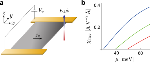
Here we argue that, aside from determining the band topology, the distorted crystal structure of 1T’-WTe2 (Fig. 1a-c) also enables unusual bulk band quantum geometry and spin physics to be accessed and controlled. By developing a low energy model from symmetry analysis we find that when an out-of-plane electric field is applied, spin-degeneracy is lifted (Fig. 1d,e) by inducing both in-plane as well as out-of-plane spin orientations (Fig. 2a,b). While in-plane spin orientations are synonymous with an out-of-plane inversion symmetry (IS) breaking, out-of-plane spin orientations are less common and typically weak Yuan . As we discuss, 1T’-WTe2 bucks this expectation: even though is out-of-plane, the non-aligned outer Te atoms (Fig. 1c) enables an in-plane electric dipole to develop and a strong out-of-plane spin orientation to be induced.
Crucially, applied induces Berry curvature as well as magnetic moment. Berry curvature value is determined by an interplay between strong atomic (spin-selective) inter-orbital mixing of the 1T’-WTe2 and induced terms, and exhibits a characteristic anisotropic distribution; magnetic moment mirrors this behavior (see Fig. A-2). While an electrically tunable Berry curvature can be readily realized in bilayer systems Xiao07 owing to a electric control over layer degree of freedom, electrical tunability in monolayer systems is considerably more difficult. Berry curvature is realizable in 1T’-WTe2 as a direct result of the asymmetric non-aligned outer Te atoms.
Further, due to the low symmetry of 1T’-WTe2 distorted crystal structure, induced Berry curvature and magnetic moment also possess an asymmetry characterized by a dipolar distribution in reciprocal space. As a result, shifts in the distribution function (e.g., induced when a dissipative charge current is flowing, ) enable a net Berry flux, and a net out-of-plane magnetization, , to develop (Fig. 4). The latter corresponds to a direct (linear) magneto-electric effect (), where characterizes the strength of the magneto-electric effect; the former mediates a quantum nonlinear anomalous Hall effect Sodemann .
Both these are intimately tied to the low-symmetry of gated 1T’-WTe2; they do not appear in rotationally symmetric systems. They constitute striking experimental signatures of the tunable quantum geometry (induced Berry curvature and magnetic moment) of 1T’-WTe2, as well as the direct impact that its distorted structure has on its material response. Using available parameters for 1T’-WTe2, we anticipate a sizeable that can be readily probed for e.g., using Kerr effect microscopy lee2017 . 1T’-WTe2 provides a compelling venue to manipulate spins and magnetic moments in a tunable two-dimensional material. Out-of-plane spin orientations are particularly useful since they may enable to couple to out-of-plane spins necessary for high-density magnetic applications MacNeil ; Kurebayashi .
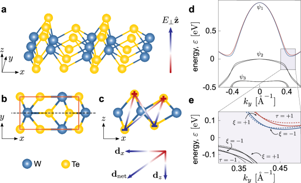
Symmetry analysis and model — We begin by analyzing the band structure of monolayer 1T’-WTe2 in the presence of an applied out-of-plane electric field [Fig. 1(a)]. In doing so, we will employ a method based on the underlying symmetries of the material: for e.g., mirror symmetry about the mirror plane [dashed line in Fig. 1(b)], time-reversal symmetry (TRS), and (broken) inversion symmetry (IS). For completeness, our analysis takes into account the three relevant atomic orbitals () and two spin states () that contribute to the states near the point and the gap opening [Fig. 1(d)], as revealed by ARPES measurements Tang as well as first principles calculations Qian ; Choe ; Lin ; Xu . This produces a six-band description (SBD), see Appendix Supp , for a detailed account of the symmetry analysis of these orbitals and spin operators and the symmetry allowed terms in the SBD description.
Importantly, while produces a spin-degenerate bandstructure Tang ; Qian ; Choe ; Lin ; Xu , when (e.g., induced by proximal gate) we find the bands become spin-split (Fig. 1d). As shown in Fig. 1d, this is particularly relevant away from the point, where the splitting becomes pronounced close to the band gap (gray shaded region, Fig. 1d,e). These are characterized by states with higher () or lower () energies as shown in Fig. 1e, and correspond to the conduction and valence bands. As we will see, the splitting induced by drives a range of novel spin behavior.
At low carrier densities typical for 1T’-WTe2 devices Wu , the electronic and spin behavior is dominated by low-energy excitations around the bandgap in the four bands (Fig. 1e). In order to compactly illustrate the physics, we develop a simple effective four-band model using the basis , , , in the regime around the gap opening (see gray region). This is obtained by performing a Löwdin partitioning (see Supp ) of the bands in Fig. 1d and can be expressed as . Here describes the electronic behavior in pristine 1T’-WTe2 ():
| (5) |
where , , represents the strong spin selective atomic orbital coupling (sharing the same spin), while and are diagonal parts for the conduction and valence bands, capturing their energy offsets and effective masses Supp . We note that is simply a tilted Bernevig-Hughes-Zhang (BHZ) hamiltonian Bernevig that describes the spin-degenerate bands in pristine 1T’-WTe2; here the tilt arises from large effective mass differences between the conduction and valence bands (see Table. A-III Supp ).
On the other hand, captures the electric field-induced spin-orbit coupling that are allowed by symmetry
| (6) |
where we have grouped the electric field-induced spin-orbit coupling terms into and in order to highlight the out-of-plane and in-plane spin orientations they induce respectively (see Fig. 2). Here , are -independent coupling terms, and is a -dependent that can induce out-of-plane spin orientation. We note, parenthetically, that the spin-orbit coupling terms in have sometimes been referred to as “Zeeman-like” see e.g., Ref. Yuan ; Xu so as highlight the out-of-plane spin orientation it induces; in the following, we will not use this terminology, but instead focus on their physical manifestation: its spin orientation. We emphasize that both and in this work physically originate from IS breaking induced by the application of the electric field, see next section for detailed discussion.
In writing Eq. (6) we have kept all symmetry allowed terms up to the linear order in as allowed by symmetry. We remark that the magnitudes of each of the symmetry allowed terms can be determined from experimental or first principle calculation results (see Appendix Supp for a discussion). However, before we move to specific values, we first discuss the physical origin of the coupling terms, and some possible interplays brought by these couplings.
Physical origin of out-of-plane and in-plane spin orientations — For physical clarity, we will denote and as spin-orbit coupling induced by out-of-plane and in-plane IS breaking, respectively. In a general sense, [or ] always couple states with opposite spins [the same spin]. As a result, these terms split the spin degeneracy and re-orient the spins of the eigenstate : terms create in-plane spin orientations (Fig. 2a) whereas terms align spins out-of-plane (Fig. 2b). Here spin orientations are plotted only for the right valley (). For , spin textures are flipped.

Their physical origins are also distinct. When a charge neutral monolayer 1T’-WTe2 is placed under , the top layer and the bottom layer Te atoms experience a charge redistribution becoming oppositely charged. This charge redistribution counteracts forming an out-of-plane dipole moment, (see Fig. 1c). Crucially, because the Te atoms are not perfectly aligned, this charge redistribution also creates an in-plane electric dipole moment along the -direction, , yielding a net induced electric dipole, , that is canted (see Fig. 1c).
As a result, induces IS breaking in both - and -directions developing a nonzero and ; here is the local electro-static potential induced by . Since spin-orbit coupling arises as matrix elements of the microscopic spin-orbit interaction: 111see e.g., Eq. (16.1) of Ref. Bir , or Eq. (2.4) of Ref. WinklerBook , we find that spin-orbit coupling terms and come from the total out-of-plane electric field ; this constrains the terms and in to be in-plane only. However, the charge re-distribution also enables an in-plane to develop. This in-plane electric field picks out in as the out-of-plane component , and as the -component. As a result of the in-plane , terms and in Eq. 6 manifest. The distorted structure of 1T’-WTe2 enables that is generically canted with finite and terms that co-exist. In contrast, since and result from the in-plane electric field , the non-distorted transition metal dichalcogenide monolayers whose atoms at top and bottom layers are aligned (e.g., MoS2) do not possess an external -induced out-of-plane spin orientations near the point (up to linear in ).
As a further illustration of the role that low symmetry plays in 1T’-WTe2, we can also compare the spin-orbit coupling terms in allowed in 1T’-WTe2 [induced by out-of-plane IS breaking], with that of HgTe quantum wells recently discussed in the literature Tarasenko ; Rothe . For 1T’-WTe2, all terms in are allowable when an out-of-plane electric field is applied because of its very low symmetry, and that fact that angular momentum in the -direction is not a good quantum number. In contrast, HgTe quantum wells possess a symmetry, is missing because its 2nd and 4th basis functions are heavy hole bands with and the coupling between them is at least of order. Only and can appear, corresponding to the existence of bulk inversion asymmetry Tarasenko and structural inversion asymmetry Rothe , respectively.
Interplay between Berry curvature and the two types of spin-orbit couplings — Pristine 1T’-WTe2 possesses both IS and TRS ensuring that Berry curvature (and orbital magnetic moment) vanish exactly. As we now discuss, in 1T’-WTe2 with , [Eq. (6)] presents an opportunity to break in-plane IS turning on a finite Berry curvature distribution. For clarity, we will first focus on the case when and are non-zero, while setting the -independent terms , and then analyse the case when later in the text.
To proceed, we first note that for pristine 1T’-WTe2 (when ), the hamiltonian in Eq. (5) possesses spin degenerate states , with corresponding to states, and spin-degenerate energy where is the energy difference between the conduction and valence bands. In the absence of , conduction () and valence () bands touch, and exhibit a gapless spectrum along - Muechler . However, large spin-selective atomic orbital coupling in 1T’-WTe2 creates strong inter-orbital mixing (between ) giving a large QSH gap Tang .
Even though the external induced spin orbit coupling [Eq. (6)] is small as compared with the intrinsic spin-selective atomic orbital coupling, , nevertheless, when an external electric field is applied, IS is immediately broken. Specifically, we emphasize that it is in-plane IS breaking that enables a finite Berry curvature, , distribution to develop. As a result, we find that encoding in-plane IS breaking (arising from , Fig. 1c) turns on . In contrast, while is also induced by (and can also spin-split bands) it corresponds to an out-of-plane IS breaking, and does not lead to .
To see this explicitly, we first consider the case where out-of-plane IS breaking is much weaker than in-plane IS breaking. In this case, dominates and we can take . Therefore, produces a bandstructure with a lifted spin-degeneracy (Fig. 1e) and energies . We note that since both as well as spin-selective atomic orbital coupling do not mix spins, possess spins that purely point out of plane (Fig. 2b). Using this, we find a Berry curvature distribution as
| (7) |
Strikingly, in Eq. (7) does not depend on even though finite was required to break in-plane IS. Instead, is solely determined by the spin-selective atomic orbital coupling , and the band parameters in pristine 1T’-WTe2.
This decoupling behavior between IS breaking strength and the value of persists even in the presence of finite out-of-plane IS breaking characterized by the ratios . To see this, we note that when is finite, starts to hybridize with different spins (in the same band). Since the intrinsic Berry curvature for spin up and spin down states are opposite in sign, when the states couple (via ) the Berry curvature drops. Along the high symmetry line about which the Berry curvature is even due to the TRS and mirror symmetry in the -direction, the Berry curvature for the spin split bands near band edge can be expressed as Supp
| (8) |
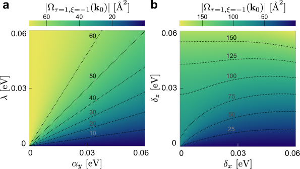
clearly displaying how tends to the value expected in for . In Fig. 3a, we plot the peak value of Berry curvature reproduced in a numerical evaluation of the SBD description. This verifies our above analysis that the value of is bounded by the intrinsic (depends only on ) , and is tuned only by the ratios , which makes equi-Berry-curvature contours to be straight lines (see Fig. 3a).
We now consider the case of , while setting -dependent terms . By numerically evaluating peak Berry curvature (see Fig. 3b), we find that the peak Berry curvature develops a more complicated behavior. In particular, is no longer bounded by the intrinsic value , and increases with without saturation. However, similar to the previous case, out-of-plane IS breaking alone is not able to induce a nonzero Berry curvature since it corresponds to an out-of-plane IS breaking. Large Berry curvature only appears when is significant.
In the above, we concentrated on unveiling the (Berry curvature) features that the various symmetry allowed spin-orbit coupling terms possess. These features can in turn help to diagnose which of the (a priori symmetry-allowed) spin-orbit coupling terms dominate. We illustrate this by comparing with recent first principles calculations as well as a recent experiment Xu . In Ref. Xu , the Berry curvature of monolayer 1T’-WTe2 was investigated at different perpendicular electric fields, from 0 to around 1 V nm-1 using both first principles and a photocurrent measurement. In particular, their first principles results revealed the induced spin-splitting in the bandstructure that vanished at larger away from the band edge, and a peak Berry curvature that increased with . This observation means that -dependent spin-orbit couplings may play only a minimal role. Further both the experiment and the first principles calculations found large Berry curvature at band edge even at small electric field shows that (see Fig. 3). Strikingly, these values of Berry curvature are close to the large intrinsic values expected from and . Together with Fig. 3b this indicates that the in-plane IS breaking and terms dominates, overwhelming the terms. As a result, in what follows we will use the k-independent spin-orbit coupling term to describe the induced spin texture.
Current induced magnetization — Another closely related quantity, the (intrinsic) orbital magnetic moment , also appears when in-plane IS is broken by :
| (9) |
where we have written as a short-hand, and is the hamiltonian. The orbital magnetic moment comes from the self-rotation of a Bloch electron wave packet around its center of mass, and is an intrinsic property of the Bloch band Xiao , and its distribution in momentum space mimics that of the Berry curvature distribution (see Appendix Supp ).
The low-symmetry of 1T’-WTe2 enables an asymmetric distribution of of and (see Fig. 4 a,b). This affords the opportunity to realize Berry phase effects not normally achievable in their rotational symmetric cousins. A striking example is the (linear) magneto-electric effect (ME) (), where the flow of an in-plane current induces an out-of-plane magnetization. While typically found in multi-ferroic materials Eerenstein where TRS and IS are explicitly broken, ME effects can arise in metals with sufficiently low symmetry (broken IS as well as broken rotational symmetry) and where the dissipation of a charge current breaks TRS Levitov . 222 We can see these from the symmetry analysis as follows: (a) in a time-reversal symmetric system , then under the symmetry operation we have , , and which leads to ; (b) if a system has a rotational symmetry, then under the rotation by angle we have , , , and which leads to (), i. e., rotational symmetry is not allowed for non-zero and ; (c) if a system is centrosymmetric, then under the operation we have , , and which also requires . . This is termed the kinetic ME effect Levitov ; Sahin .
Indeed, the low-symmetry of 1T’-WTe2 (with ) where only a mirror symmetry in the -direction remains is the largest symmetry group that hosts the kinetic ME Levitov ; Sodemann . This makes 1T’-WTe2 a natural venue to control ME.
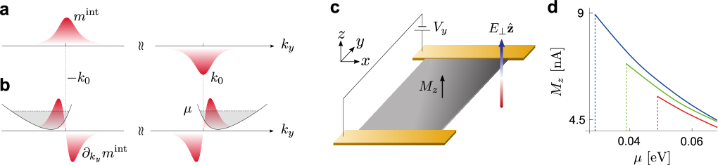
To illustrate the kinetic ME effect in 1T’-WTe2, we first note that the magnetic moment is asymmetric, displaying a dipolar distribution (see Fig. 4a,b). This can be seen explicitly by considering and noting that it is displaced in relation to the bottom of the band, Fig. 4b. As a result, when an in-plane electric field shifts the distribution function, a uniform out-of-plane magnetization develops:
| (10) |
where is the Drude weight along direction, is the equilibrium distribution function, is the intrinsic contribution to the magnetic moment in a particular band, containing both orbital and spin contributions with . For 1T’-WTe2 monolayer, we estimate Wu ; Fei .
Importantly, Eq. (10) reflects the symmetry of the crystal. For example, magnetic moment distribution has equal magnitudes but opposite signs in the two electron pockets in the conduction band. As a result, vanishes as expected from symmetry, see above. In contrast, when in-plane electric field is applied along , a non-zero is generated (i.e. ).
Using Eq. (10), we obtain a finite out-of-plane magnetization in Fig. 4d when current is driven along the direction. In doing so, we used with the chemical potential, and computed the Drude weight in the usual fashion. Further, to capture the full reciprocal space distribution of the magnetic moment (including regions away from the gap opening), we used the SBD description to compute the magnetic moment distribution. Here we have concentrated on small chemical potentials so that only moments in the lowest conduction band (blue band in Fig. 1e) contribute. Since is an odd function of when TRS is present, the filled bands do not contribute to ME. This reflects the fact that kinetic ME arises from a dissipative process. As a result, when the chemical potential is in the gap, . However, once the system is doped into the conduction band, a non-zero ME develops, see Fig. 4d. Similar analysis also applies to the Berry curvature (which exhibits a dipolar distribution), and leads to a non-linear Hall effect without applied magnetic field (see Ref. Sodemann as well as the Appendix Supp for an explicit discussion for this system).
Summary – 1T’-WTe2 with an applied out-of-plane electric field , provides a new and compelling venue to control bulk band quantum geometry. In particular, its bands exhibit a tunable Berry curvature and magnetic moment with switch-like behavior. Crucially, the low symmetry of its crystal structure enable effects not normally found in its rotationally symmetric cousins. These include striking Berry phase effects such as a current induced magnetization (ME), and a quantum non-linear Hall effect. These are particularly sensitive to orientation of in-plane electric field and the crystallographic directions. Indeed, is strongest when current runs along the -direction; this sensitivity can be verified through measurements in a single 1T’-WTe2 sample, for e.g., using a Corbino disc geometry. Perhaps most exciting, however, is how IS broken 1T’-WTe2 enables direct and electric-field tunable access to out-of-plane magnetic degrees of freedom. Given its two-dimensional nature, 1T’-WTe2 can be stacked with other two-dimensional materials, providing a key magneto-electric component in creating magnetic van der Waals heterostructures.
Acknowledgements - We gratefully acknowledge useful conversations with Valla Fatemi, Qiong Ma, Su-Yang Xu, and Dima Pesin. This work was supported by the Singapore National Research Foundation (NRF) under NRF fellowship award NRF-NRFF2016-05 and a Nanyang Technological University Start-up grant (NTU-SUG).
References
- (1) X. F. Qian, J. W. Liu, L. Fu, L. Li, Science 346, 1344 (2014).
- (2) S. J. Tang et al., Nat. Phys. 13, 683 (2017).
- (3) Z. Y. Fei et al., Nat. Phys. 13, 677 (2017).
- (4) S. F. Wu, V. Fatemi, Q. D. Gibson, K. Watanabe, T. Taniguchi, R. J. Cava, P. J. Herrero, Science 359, 76 (2018).
- (5) H. T. Yuan et al., Nat. Phys. 9, 563 (2013).
- (6) D. Xiao, W. Yao, Q. Niu, Phys. Rev. Lett. 99, 236809 (2007).
- (7) I. Sodemann, L. Fu, Phys. Rev. Lett. 115, 216806 (2015).
- (8) J. Lee, Z. F. Wang, H. C. Xie, K. F. Mak, J. Shan, Nat. Mater. 16, 887 (2017).
- (9) D. MacNeill, G. M. Stiehl, M. H. D. Guimaraes, R. A. Buhrman, J. Park, D. C. Ralph, Nat. Phys. 13, 300 (2017).
- (10) H. Kurebayashi, Nat. Phys. 13, 209 (2017).
- (11) See Appendix for discussions of the six-band description and symmetry analysis, reduction to a effective Hamiltonian, Berry curvature at the band edge, Berry curvature and magnetic moments for non-zero distribution in momentum space, and quantum non-linear anomalous Hall effect.
- (12) D. H. Choe, H. J. Sung, K. J. Chang, Phys. Rev. B 93, 125109 (2016).
- (13) X. Q. Lin, J. Ni, Phys. Rev. B 95, 245436 (2017).
- (14) B. A. Bernevig, T. L. Hughes, S.-C. Zhang, Science 314, 1757 (2006).
- (15) L. Muechler, A. Alexandradinata, T. Neupert, R. Car, Phys. Rev. X 6, 041069 (2016).
- (16) D. Xiao, M. C. Chang, Q. Niu, Rev. Mod. Phys. 82, 1959 (2010).
- (17) W. Eerenstein, N. D. Mathur, J. F. Scott, Nature 442, 759 (2006).
- (18) L. S. Levitov, Y. V. Nazarov, G. M. Eliashberg, Sov. Phys. JETP 61, 133 (1985).
- (19) C. Şahin, J. Rou, J. Ma, D. A. Pesin, Phys. Rev. B 97, 205206 (2018).
- (20) R. Winkler, U. Zülicke, Phys. Rev. B 82, 245313 (2010).
- (21) M. Zhou, R. Zhang, J. P. Sun, W. K. Lou, D. Zhang, W. Yang, K. Chang, Phys. Rev. B 96, 155430 (2017).
- (22) G. L. Bir, G. E. Pikus, Symmetry and Strain-Induced Effects in Semiconductors (Wiley, New York, 1974)
- (23) R. Winkler, Spin-Orbit Coupling Effects in Two-Dimensional Electron and Hole Systems (Springer, Berlin, 2003)
- (24) S.-Y. Xu et al., Nat. Phys. 14, 900 (2018).
- (25) S. A. Tarasenko, M. V. Durnev, M. O. Nestoklon, E. L. Ivchenko, J. W. Luo, A. Zunger, Phys. Rev. B 91 081302 (2015).
- (26) D. G. Rothe, R. W. Reinthaler, C. X. Liu, L. W. Molenkamp, S. C. Zhang, E. M. Hankiewicz, New Journal of Physics, 12 065012 (2010).
Appendix for “Symmetry, spin-texture, and tunable quantum geometry in WTe2 monolayer”
.1 Six-band model for monolayer 1T’-WTe2
Without external fields, 1T’-WTe2 monolayers possess time-reversal (TR) symmetry and a point symmetry group that contains four symmetry operations. If we set one of the inversion center as the origin in real space, the four symmetry operations are where denotes shifting by a unit cell in the -direction. When we shift the origin to , the four symmetry operations become .
Various first-principle calculations as well as expermental measurements Qian ; Tang ; Choe ; Lin showed that there are three relevant orbitals contributing to the states near the gap. Although the exact orbital compositions at the point is not clear, these orbitals at the point are consistently revealed Tang ; Choe ; Lin to be (even, odd, even) under the reflection operation in -direction (the orbitals are ordered with decreasing energy). Here we note that Choe et al. used a different coordinate system with and directions exchanged.
A perpendicularly applied electric field breaks symmetry operations that flip in the -direction and reduce the point group to group that has only two symmetry operations (i. e., identity and reflection about the plane that cross a Te atom). It has two real 1D irreducible representations (see Table A-I).
Aside from the spin degrees of freedom, each of the three orbitals at the point is non-degenerate and transforms according to one of the 1D irreducible representations of . Moreover, although inversion symmetry is broken, the three orbitals remain (even, odd, even) in the -direction at the point. These two observations show that the three orbitals at the point transform as:
| (A-1) |
where the symbol “” denotes how these functions transform under operations in . Using , , as basis, the Hamiltonian near the point assumes a form:
| (A-5) |
where is the () block matrix between and with (without) spin degree of freedom included.
In the following, we will obtain the general form of from symmetry analysis. The necessary information for is contained in its transformation property under group [Eq. (A-1)]. We note that detailed orbital compositions, e. g., the weight of - or - orbital in , does not affect the following analysis.
We will proceed by using the theory of invariants Bir ; Winkler ; Zhou which is based on the invariance of the Hamiltonian under all operations of the corresponding crystal symmetry group. When the Hamiltonian is projected to the energy bands of interest , where denotes a tensor operator formed by combinations of wave vectors, the symmetry group constrains the Hamiltonian as follows: under an arbitrary symmetry operation , the basis transforms according to the irreducible representation , so the invariance of the Hamiltonian under the symmetry operation dictates , where denotes the operator for symmetry operation . This leads to , or equivalently,
| (A-6) |
where with is the representation matrix of in (in the 1D irreducible representation case here, or ), and denotes the transformation of under the symmtery operation , e. g., if and , then .
In constructing the operators, one can also take into account the spin degree of freedom, by including the spin operator in the Hamiltonian. Note that is a pseudovector, we have , , and under the operation Zhou , e. g., if and , then .
For general cases in which crystals have high symmetry point groups, the expression of an arbitrary block of the Hamiltonian can be constructed in several standard procedures with the corresponding full character table Bir ; Winkler ; Zhou . In our case, however, the group is the simplest non-trivial group that has only two symmetry operations , and we can do the analysis just based on mirror symmetry operation :
i) For blocks () and : since () and are even under operation, to make sure is invariant under operation, then () and must be composed by operators that are also even under operation. Relevant operator combinations that are invariant under operation are listed in the first row of Table A-I.
| TR invariant operators | |||
|---|---|---|---|
| , , , , , , , | |||
| , , , , , |
ii) For blocks and : since and are odd under operation, then and must be composed by operators that are also odd under operation to ensure that is invariant under operation. Relevant operator combinations that are odd under are listed in the second row of Table A-I.
After obtaining the terms that transform correctly for each of the blocks, we note further constraints that trim the Hamiltonian:
(1) The Hamiltonian must be Hermitian, which dictates that the invariants for a diagonal block must be Hermitian.
(2) Terms containing both and are matrix elements of the microscopic spin-orbit interaction in thus terms and will not appear.
(3) For our purposes of estimating the Berry curvature and orbital magnetic moments in the main text, we can neglect the block. This is because and are energetically far away from each other ( eV) and their couplings only have small contributions to Berry curvature and orbital magnetic moment for the conduction bands. Although block contributes to optical transitions eV, this is beyond our current scope.
The above three considerations trim/eliminate the terms . For remaining terms, we group them into terms induced by the applied perpendicular electric field, and those that are present in pristine 1T’-WTe2. To do so we perform the following symmetry analysis: when the electric field is not present, inversion symmetry about the inversion center is recovered, and the operation about becomes a symmetry operation again. Under the operation , there is no flip in the -direction while and . We can see that terms change sign under this new operation, i. e., they are not invariant under the original symmetry group and can appear only when the perpendicular electric field is applied.
| , | ||
|---|---|---|
| with or w/o | , , | , |
| with | ; , | ; |
After trimming, classification, and analyzing the physical origin of the terms induced by electric field, we now obtain the general form of the Hamiltonian (see Table A-II).
First we use a least squares fitting to extract coefficients of these invariant operators from known band structure, either from experimental measurements or numerical calculations. From the first principle calculation result Qian ; Xu , we obtained the Hamiltonian when there is no external fields. We find
| (A-13) |
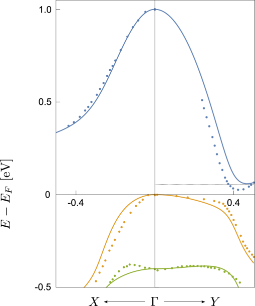
where , and . The dispersion is plotted in Fig. A-1, with parameters listed in Table A-III.
| Parameter | Value | Unit | Parameter | Value | Unit |
|---|---|---|---|---|---|
| eV | |||||
| eV | |||||
| eV | |||||
| eV Å2 | eV Å2 | ||||
| eV Å2 | eV Å2 | ||||
| eV Å2 | eV Å2 | ||||
| eV Å | eV Å | ||||
| eV Å | eV Å |
The additional terms that are induced by the applied perpendicular electric field makes the full Hamiltonian , with
| (A-20) |
where is the commonly seen spin-orbit coupling for -th orbital (this is sometimes referred to as “Rashba” spin texture), is a spin splitting from in-plane IS breaking, and and are -independent inter-band couplings, see main text for discussion of physical origin.
.2 model near the band gap
To obtain the effective Hamiltonian near the band gap, we consider the energy eigenvalue equation
| (A-27) |
where () is the () diagonal block from the original Hamiltonian, and () is the corresponding four (two) component state vector, and is the matrix couples and .
The second row of Eq. (A-27) allows to be written in terms of :
| (A-28) |
Substituting this into the first row of Eq. (A-27) gives an effective eigen equation solely for the components:
| (A-29) |
Performing the standard expansion in small as well as rotation procedure Winkler , we obtain the effective Hamiltonian near the band gap as
| (A-30) |
valid when is small, and we have used the rotated basis .
Following the above analysis, we now derive the model for the pristine part. From Eq. (A-13) we have
| (A-35) |
| (A-38) |
and
| (A-41) |
where , and . Using and above, we have
| (A-46) |
where , and
| (A-47) |
Here the -dependent ratio is
| (A-48) |
which controls the renormalization of and . It becomes zero when , i. e., when and do not couple with each other, and there is no renormalization. We note that the form of this pristine part in Eq. (A-46) is consistent with the model proposed in Ref. Qian ; for a full discussion see the section “Unitary transformation and form of Hamiltonian” below.
If we re-order the basis to , ; , , this gives the BHZ-type pristine part,
| (A-53) |
where , . Together with the electric field induced part (neglecting the far away band),
| (A-58) |
we obatined the effective hamiltonian near the gap opening
| (A-59) |
When focusing on the dispersions and Berry curvatures near the gap opening, we find a convenient estimate for :
| (A-60) |
where is the position of the band edge with . By doing this, we obtained the dispersion and a Berry curvature distribution which agree well with the six band model near the gap opening (see solid and dashed lines in Fig. 1d and Fig. 1e for comparison).
.3 Berry curvature at the band edge from model
( case)
Using the band model [see Eq. (5) and Eq. (6) of the main text] to describe 1T’-WTe2, we can express its Berry curvature near the band edge analytically.
Without the electric field induced part , the BHZ-type pristine part can be viewed as two decoupled blocks: spin-up block and spin-down block . The two blocks form a time-reversal pair
| (A-63) |
where . The two blocks share the same dispersion relation and are spin-degenerate:
| (A-64) |
with the corresponding eigenstates:
| (A-65) |
where denotes conduction or valence band, and is the energy difference between the conduction and valence bands.
When an external perpendicular electric field is applied and if the spin-orbit couplings induced by the field is much weaker than the atomic spin-orbit couplings (), we then treat as a small perturbation to the pristine part . We first note that for non-zero , and within the framework of degenerate perturbation (i.e. neglecting states that are far away in energy), hybridizes the unperturbed spin up state and spin down state in the same band into spin split states , with higher () or lower () energies:
| (A-66) |
Interestingly, in the limit, the unperturbed spin up state and spin down state do not hybridize with each other. Even so, their degeneracies are lifted by :
| (A-67) |
The Berry curvatures for these non-degenerate states are well defined and read
| (A-68) |
When , spin up state and spin down state start to hybridize to form the spin split states . The Berry curvature amplitudes for these hybridized states are smaller than that of because the spin up and spin down states have opposite Berry curvatures.
The general form of the Berry curvature for is complicated. Fortunately, along about which the Berry curvature is even, i. e., , which comes from the TRS and the mirror symmetry in the -direction, its analytical form is greatly simplified:
| (A-69) |
where and satisfy
| (A-70) |
With this, the Berry curvature at the band edge is
| (A-71) |
.4 Berry curvature and magnetic moment distribution
(,
case)
Here we show the anisotropic Berry curvature and magnetic moment distribution in -space away from the gap opening, using the six band description (SBD) we developed (see Fig. A-2). The formula for calculating Berry curvature and moment distribution are
| (A-72) |
| (A-73) |
where is the short-hand form, and is the full six band hamiltonian.

.5 Non-linear anomalous Hall effect
Just as discussed in the main text gives rise to ME, in the bands enable 1T’-WTe2 to exhibit a quantum non-linear Hall effect at zero magnetic field. This can be seen under general symmetry considerations Sodemann . For the convenience of the reader, we outline this symmetry analysis for a 2D system that only has in-plane mirror symmetry (e.g., 1T’-WTe2). The non-linear Hall current can be written as (). Under the operation , we have and . This allows a non-zero (while vanishes). Under an in-plane DC electric field, can be obtained using Sodemann
| (A-74) |
where is the transport scattering time. Similar to Eq. (10) above, is an odd function of [see Fig. A-2(a)]. As a result, nonzero only occurs when and : only electric field along induces a non-linear Hall effect along . When is parallel to the -direction, the nonlinear Hall effect (as well as the kinetic ME effect) vanishes.
To illustrate the quantum non-linear Hall effect, we numerically integrate Eq. (A-74) to obtain a finite non-linear Hall current conductivity in Fig. A-3b using a scattering time . Similar to in the main text, we used the SBD description in order to capture the full reciprocal space distribution of the Berry curvature. This non-linear Hall conductivity can be probed in a conventional Hall bar measurement (Fig. A-3) and provides a fully electrical way of mapping the Berry curvature (dipole).
.6 Unitary transformation and form of Hamiltonian
We note that the model in the supplement of Ref. Qian is equivalent to our model for the pristine part. For the convenience of the reader, we reproduce the four band hamiltonian in Ref. Qian as
| (A-79) |
To see the equivalence, we use the unitary transformation
| (A-84) |
Applying the unitary transformation, we have
| (A-85) |
reproducing Eq. (A-46).