Symplectic Effective Field Theory for Nuclear Structure Studies

The simplest Lagrangian density one can write for a real scalar field $\varphi$ is

which is the Lagrangian density of a harmonic oscillator (HO) for massless excitations (bosons). The classical, still not quantized, fields that satisfy the equations of motion of this Lagrangian are given by the plane-wave solution.

The integration is over four variables, the three momenta (k, a spatial vector) and the energy (E, a scalar). The construction of the effective field theory is accomplished by taking the Lagrangian in Eq. (1) and extending it naturally to its $n$-th order and adding a mass term at every order,

The total Lagrangian density is $\mathcal{L}=\sum_{n}\mathcal{L}^{(n)}$, where for the $n=0$ term we recover Eq. (1). We have added a term $nm^{2}\varphi^{2}$, often called “the mass” term, at every order. This is added to capture all possible combinations of interaction terms that could result from lowest powers of $\varphi$ and $\partial_{\mu}\varphi\partial^{\mu}\varphi$. Including $\varphi$ only shifts the equations of motion by a constant, therefore the lowest possible power is $\varphi^{2}$. In this formulation $\alpha$ is the coupling coefficient of the theory. Since the dimension of a Lagrangian density always has to be $[\mathcal{L}]=4$, it follows logically that $[\alpha]=-4$ and as well that this is a non-renormalizable EFT. The main advantage of this systematic construction of the Lagrangian density given by Eq. (3) is that it is unique in the sense that the plane wave solution given by Eq. (2) satisfies the equations of motion at every $n$-th order without the need to consider perturbative corrections if one imposes a specific condition on $\alpha\sim 1/N^{3/2}_{av}$, where $N_{av}=\sqrt{N_{f}N_{i}}$ is the geometric average of the total number of excitations (bosons) between the initial $\ket{N_{i}}$ and final $\ket{N_{f}}$ Fock states that the interaction is acting on, as shown in Appendix (A). At $n=0$ the excitations (bosons) are massless with energy $|E_{k}|=|\textbf{k}|$ and for any arbitrary $n>0$ a mass-like term is introduced through the self interaction that turns out to be the main driver of a $Q\cdot Q$ quadrupole-quadrupole type interaction. This, alongside the imposed condition on $\alpha$, allows us to include all terms up to an arbitrary $n$-th order.

The EFT has to be suitable for describing nuclei, and therefore it is necessary to use discretized fields instead of Eq. (2), through localized plane waves within cubic elements of volume $V$ with periodic boundary conditions. This condition requires that the plane waves have the following discrete form:

where $b^{+}_{\textbf{k}}$ creates an excitation (boson) and $b_{\textbf{k}}$ destroys an excitation (boson), respectively, with energy $|E_{k}|=|\textbf{k}|$ by acting on a $\ket{N_{k}}$ state, where $N_{k}$ is the number of excitations (bosons) with momentum k.

Now that we have identified the required fields and operators, we need for them to describe excitations of a system of $\mathcal{A}$ nucleons, which means the fields must enter pair-wise (quadratically, to preserve the parity of each single-nucleon wave function), and therefore for a nucleus with $\mathcal{A}$ nucleons the Lagrangian density given in Eq. (3) has to be generalized to

which is the Lagrangian density of an $\mathcal{A}$-component real scalar field and is O$(\mathcal{A}-1)$ symmetric [$(\mathcal{A}-1)$ to remove the center-of-mass contribution]. It has been established that the symplectic Sp(3,R) group is a complementary dual of the O$(\mathcal{A}-1)$ symmetry group [32]. This implies that the Lagrangian itself is part symplectic, meaning that the resulting quantum mechanical Hamiltonian from it, after making specific couplings, preserves symplectic symmetry and doesn’t mix configurations belonging to different symplectic irreps. As for the p subscript, it denotes the sum over all nucleons in the system

The symplectic symmetry is the natural extension of the SU(3) symmetry and is realized by its 21 many-body generators in their Cartesian form. Since we are constructing a 4-dimensional EFT it is appropriate to represent the symplectic generators in the interaction picture (Heisenberg representation) where the operators explicitly depend on time. This is done through

Using this definition we get the following

where the $i,j$ in subscripts denote the spatial directions and the repeated index $p$ implies a sum over the number of nucleons in the system being described. The objects $2\mathcal{Q}_{ij}=C_{ij}+C_{ji}$ are the generators of the Elliott SU(3) group that act within a major harmonic oscillator shell, whereas the symplectic raising $A_{ij}$ operator and its conjugate $B_{ij}$ lowering operator connect states differing in energy by $2\Omega$, twice the harmonic oscillator energy. The interaction picture clearly states that the symplectic operators $A$ and $B$ are the ones responsible for the dynamics (they depend on time) in nuclei that can be interpreted as vibrations in space and time. Whereas the $C$ operators (independent of time) are responsible for the static deformed configurations in nuclei that can rotate freely. This was perhaps implicitly evident from the fact that the Sp(3,R) symmetry ($A$ and $B$) is the dynamical extension of the SU(3) symmetry ($C$), but now it is explicitly evident through their representation in the interaction picture.

To further understand the significance of these operators it is useful to define the following set of operators which are more suitable for a physical interpretation of the symplectic operators

where $Q_{ij}$ is the quadrupole tensor and is responsible for deformation, $K_{ij}$ is the the many-body kinetic tensor, $L_{ij}$ is the angular momentum tensor responsible for rotations and $S_{ij}$ is the vorticity tensor responsible for the flow of deformation.

Symplectic basis states are constructed by acting with the symplectic raising operator $A$ on the so-called band-head of the symplectic irrep $\ket{\sigma}$ which, is unique and is defined as $B\ket{\sigma}=0$ to be a lowest weight state. The band-head $\ket{\sigma}$ is mathematically similar to how the vacuum behaves $b\ket{0}=0$. However, unlike vacuum, $\ket{\sigma}$ can contain physical particles; namely, nucleons.

The complete labeling of a sympletic basis state that is constructed from its $\ket{\sigma}$ bandhead irrep is $\ket{\sigma n\rho\omega\kappa LM}$ where $\sigma\equiv N_{\sigma}(\lambda_{\sigma}\mu_{\sigma})$ labels the bandhead, $n\equiv N_{n}(\lambda_{n}\mu_{n})$ labels the excited state that, coupled to the bandhead, yields the final configuration labeled by $\omega\equiv N_{\omega}(\lambda_{\omega}\mu_{\omega})$ with $\rho$ multiplicity, $L$ angular momentum with $\kappa$ multiplicity and its $M$ projection. $N_{\omega}=N_{\sigma}+N_{n}$ is the total number of bosons (oscillator quanta), $\lambda_{a}=(N_{a})_{z}-(N_{a})_{x}$ and $\mu_{a}=(N_{a})_{x}-(N_{a})_{y}$ are the SU(3) quantum numbers, where $a=\sigma,\omega,n$. They denote the intrinsic deformation of the state since they count the difference in the number of oscillator quanta in the z and x, and x and y directions respectively. These states are ideal for describing collective features of nuclei and for serving as basis states for the EFT. Similar to the Fock state notation $\ket{N_{k}}$, symplectic basis states also describe bosons numbered by $N_{\omega}$ making them a suitable basis state to which an application of our EFT interaction yields a quantum mechanical Hamiltonian that can be utilized for carrying out nuclear structure studies.

The $n$-th order Hamiltonian density, derived in Appendix (B) is

where $\dot{\varphi}\equiv\frac{\partial\varphi}{\partial t}$ and $\varphi^{\prime}\equiv\frac{\partial\varphi}{\partial\textbf{r}}$. The total Hamiltonian density at the $n$-th order is a sum over all possible $n+1$ combinations of the $n+1$-th term in the second parenthesis in Eq. (9) with respect to the $n$ terms in the first paranthesis, therefore it is Hermitian (see Appendix (B) for proof). However, for purposes of calculating matrix elements it is sufficient to only consider Eq. (9) and then add all the possible other combinatorial terms as described.

The coupled fields in Eq. (9) are

For convenience, from here on we will drop the index $p$ denoting the sum over particle numbers from the fields since they don’t affect any of the follow-on derivations and can be recovered as may be required at any time. As evident from the formulas above the creation and annihilation operators enter into the Hamiltonian density in pairs of $b^{+}b^{+}$, $b^{-}b^{-}$, $b^{+}b^{-}$ and $b^{-}b^{+}$. This allows us to describe them through the symplectic operators defined in Eqs. (7). This definition further enables us to transition from $\ket{N_{k}}$ to $\ket{\sigma}$ where $N_{\omega}$ will be equivalent to a state with number of bosons $N_{k}$ created(destroyed) by $b^{+}_{\textbf{k}}(b^{-}_{\textbf{k}})$ with momentum k. Knowing this we can rewrite the fields in Eqs. (10) as follows:

where, for further convenience we use the notation $Z^{\pm}_{\textbf{k}}=b^{\pm}_{\textbf{k}}e^{\pm ik^{\mu}x_{\mu}}$. And finally, with these further simplifying definitions in play, the Hamiltonian density in Eq. (9) can be rewritten as follows:

where we further use the following notation:

With all of this in place, we finally come to an expression for the Hamiltonian density, $\mathcal{H}$, that enters into the integral for $H$ that we consider next.

The Hamiltonian is

Substituting $\mathcal{H}$ into the integration we notice that for every order $n$ we have $n+1$ pairs of $Z^{+}Z^{+}$, $Z^{+}Z^{-}$ and their conjugates multiplied with each other inside the integration. To demonstrate this, let us consider a term like $Z^{+}Z^{+}$ for example for the simplest case $n=0$ which gives a term like

where we absorbed the time component of the exponent into the operators. This integral is zero because of the periodic boundary condition on k and q unless $\textbf{k}+\textbf{q}=0$. To generalize for $n+1$ pairs, each term $Z^{+}Z^{+}$ and $Z^{-}Z^{-}$ has to have $\textbf{k}+\textbf{q}=0$, and each term $Z^{+}Z^{-}$ and $Z^{-}Z^{+}$ has to have $\textbf{k}-\textbf{q}=0$. We call this “diagonal coupling” because for each pair in the integral we couple k to q for example $\textbf{k}_{1}$ to $\textbf{q}_{1}$, $\textbf{k}_{2}$ to $\textbf{q}_{2}$ and $\textbf{k}_{n}$ to $\textbf{q}_{n}$, etc. The result of this simple coupling is that each $\mathcal{Z}$ term in Eq. (12) doesn’t interact with other similar terms, meaning the sums don’t mix with each other inside the integral, which leads to the Hamiltonian presented in Eq. (17), below. (See Appendix (C) for this derivation,)

Comparing the terms in the Hamiltonian to the symplectic operators defined in Eq. (7) it is straightforward to see that this Hamiltonian is symplectic in nature because, for example, $b^{-}_{\textbf{k}_{1}}b^{-}_{-\textbf{k}_{1}}$ is simply $b^{-}_{i}b^{-}_{i}$ which is the symplectic lowering operator $B_{ii}$ after we recover the sum over particle number $p$. This implies that symplectic symmetry emerges naturally from the EFT Lagrangian in Eq. (3) whose sole construction was done naturally by extending the harmonic oscillator Lagrangian out to its $n$-th order. This implies that symplectic symmetry is an extension of the SU(3) symmetry of the harmonic oscillator which algebraically was known and well understood through nuclear physics applications but here, as seen through these developments, symplectic symmetry in nuclear physics has its origin at a more fundamental level than previously considered; specifically, it derives from and is underpinned by a logical EFT formulation.

In this effective field theory for determining the structure of atomic nuclei the nucleons in a nucleus are represented through the total energy quanta (bosons) they bring forward, which in turn can be created and destroyed at all possible energy values. This can be envisioned as having an infinite quantum mechanical harmonic oscillator systems, each with $E_{k}$ wherein the nucleons are contained. Such excitations are constrained to a very narrow range of possible energy values. Studies done with mean field models and also realistic interactions all support such a claim, as do calculations using the NCSpM [31] and SA-NCSM [40]. Specifically, in the latter cases, one typically finds that utilizing a single symplectic irrep suffices to recover nearly $70\%$-$80\%$ of the probability distribution, and more specifically, accounts for nearly $90\%$-$100\%$ of observables, such as energy spectra, B(E2) values and radii.

Given the fact that in all such cases the excitation quanta include only a single energy mode; $\hbar\Omega=41\mathcal{A}^{-1/3}$ MeV, the application of the Hamiltonian on a single symplectic state further reduces it to only one term, where from each sum over k survives; namely, the term where $E_{k}=\hbar\Omega$ which reduces Eq.  (17) to

This is a quantum mechanical Hamiltonian that is the natural extension to the harmonic oscillator Hamiltonian for $n\geq 1$. It represents a one-body interaction extended to an arbitrary $n$-th order. This results from the diagonal coupling discussed above and hence the $d$ subscript, and is solely responsible for generating monopole excitations in nuclei that do not contribute to the dynamics since they are just powers of $A_{ii}+B_{ii}$. They destroy the leading order harmonic oscillator at every $n\geq 1$ which is unphysical and hence they have to be removed from the final Hamiltonian. What is responsible for dynamics are vibrations in space and time due to the quadrupole excitations in nuclei that result from off-diagonal couplings in the Hamiltonian in Eq. (12). The only term from the diagonal coupling that contributes to the Hamiltonian is the harmonic oscillator which, is $H^{(0)}=\hbar\Omega C_{ii}$.

In this section, we consider two pairs of Z’s, $Z^{+}Z^{+}$, for example inside the integral resulting from multiplying two $\mathcal{Z}$ in Eq. (12), namely,

For $n=1$, which as we discussed before, this will be zero unless $\textbf{k}_{1}+\textbf{q}_{1}+\textbf{k}_{2}+\textbf{q}_{2}=0$. We managed this before by picking $\textbf{k}_{1}+\textbf{q}_{1}=0$ and $\textbf{k}_{2}+\textbf{q}_{2}=0$, etc., which resulted to the diagonal coupling. However there are many possibilities to make $\textbf{k}_{1}+\textbf{q}_{1}+\textbf{k}_{2}+\textbf{q}_{2}=0$. What is particularly interesting is if we choose $\textbf{k}_{1}+\textbf{q}_{2}=0$ and $\textbf{k}_{2}+\textbf{q}_{1}=0$. This results in a pair of $A_{\textbf{k}_{1}-\textbf{k}_{2}}A_{\textbf{k}_{2}-\textbf{k}_{1}}$ which creates a boson pair with momentum $\textbf{k}_{1}$ and $-\textbf{k}_{2}$, respectively, and creates another pair with momentum $\textbf{k}_{2}$ and $-\textbf{k}_{1}$, respectively, such that the total momentum of both pairs is conserved. If we pick $\textbf{k}_{1}=-\textbf{k}_{2}$ this will result to the diagonal coupling Hamiltonian in Eq.  (18) derived in the previous section. However we can pick $|\textbf{k}_{1}|=|\textbf{k}_{2}|$ such that $\textbf{k}_{1}\perp\textbf{k}_{2}$. This reduces $A_{\textbf{k}_{1}-\textbf{k}_{2}}A_{\textbf{k}_{2}-\textbf{k}_{1}}$ to $A_{ij}A_{ji}$ which creates two boson pairs in the $i$-th and $j$-th direction such that $i\neq j$. The same argument applies to other terms like $Z^{+}Z^{+}Z^{-}Z^{-}$, $Z^{+}Z^{+}Z^{+}Z^{-}$, $Z^{+}Z^{+}Z^{+}Z^{-}$, $Z^{-}Z^{-}Z^{+}Z^{-}$ etc.

The expression for the off-diagonal Hamiltonian depends on $n$. If $n$ is odd then we have $n+1$ even pairs of $Z^{\pm}$ that all could be coupled to each other resulting in $(n-1)/2$ identical pairs and one unique pair. If $n$ is even then we have $n+1$ odd pairs, from which we can form either $n/2$ identical pairs, and a unique pair or $(n-2)/2$ identical pairs and two unique pairs. This results in three off-diagonal Hamiltonians, one for odd $n$ and two for even $n$ for $n>0$, since for $n=0$ only diagonal coupling is possible. The resulting expressions will contain terms like $A_{ij}A_{ji}$, $C_{ij}C_{ji}$, $B_{ij}C_{ji}$ etc., which can be represented in terms of $Q_{ij}$ and $K_{ij}$ resulting into the following three two-body Hamiltonian expansions, see Appendix (D) for this derivation. The expansion resulting from the off-diagonal coupling in Eq. (12) at every $n=odd$ is

In the above equation, $g_{n}$ denotes the strength of the quadrupole operator and is tied to the mass parameter introduced in Eq. (3) (see Appendix (A) for derivation). The expansion resulting from the off-diagonal coupling in Eq. (12) at every $n=even$ is

This is one of the expansions resulting from the off-diagonal coupling in Eq. (12) at every $n=even$ and the other one is removed since every term is proportional to $A_{ii}+B_{ii}$, see Appendix (D) for additional details.

The resulting Hamiltonian for this EFT [Eq.(22)] is effectively a two parameter theory; the parameters being $\frac{\alpha}{V}\hbar\Omega$ and $g_{n}$. The parameter $\frac{\alpha}{V}\hbar\Omega=\frac{V_{\mathcal{A}}}{b^{3}N^{3}_{av}}$ establishes a clear seperation of scales. It is simply the ratio of the average spherical nuclear volume $V_{A}=\frac{4}{3}\pi R^{3}$, where $R=1.2\mathcal{A}^{1/3}$ is the average radius of the ground state, over the volume corresponding to the harmonic oscillator excitations $V=b^{3}N_{av}^{3/2}$, where $b$ is the oscillator length, along with the plane-wave condition, $\alpha\sim 1/N^{3/2}_{av}$ that allows further stretching of $V$.

If $\frac{V_{\mathcal{A}}}{b^{3}N^{3}_{av}}<<1$ the average volume of the nucleus is less than a volume determined by adding up the total number of its excitation quanta, when a plane wave solution is valid therefore preserving the harmonic oscillator structure. But if $\frac{V_{\mathcal{A}}}{b^{3}N^{3}_{av}}\sim 1$, signaling that the volume determined by adding up the number of oscillator excitations in play is approaching the average volume, a plane wave solution becomes untenable with higher order corrections becoming ever more relevant, ending in a complete breakdown when the $Q\cdot Q$ interactions destroys the HO structure. In short, as more nucleons are added to the system their corresponding boson excitations have to also increase appropriately such that they can be represented by plane waves as indicated by the $\frac{V_{\mathcal{A}}}{b^{3}N^{3}_{av}}$ measure. This further emphasizes the fact that this scale is valid as long as a shell structure description is appropriate for the systems being studied.

The second parameter of the theory is $g_{n}$ which is the strength of the quadrupole operator because only the quadrupole terms in Eq. (22) carry this parameter as a multiplier. The value of this parameter determines the strength with which the quadrupole tensor enters into any analysis relative to that of the kinetic tensor. In particular, it should be clear that if $g_{n}=0$ one gets a power series in $K_{ij}K_{ji}$. It is therefore important that the value chosen for $g_{n}>1$ for $\forall n$ is required to balance the interaction between $Q_{ij}Q_{ji}$, $K_{ij}K_{ji}$ and $Q_{ij}K_{ji}$.

The parameter $g_{n}$ is expressed in terms of the mass-like parameter introduced in Eq. (39) to represent the strength of the interaction. It results from off-diagonal couplings that depend on $n$ which has a simple physical interpretation,

The consequences of this is that the energy of the bosons contributing to the formation of a given final symplectic configuration, starting from an initial one, increases uniformly as more pairs are considered. This simple picture suggests that if $g_{1}=g$ and $g_{\infty}=2g$ then as $n\to\infty$ the weight of $Q_{ij}Q_{ji}$ will scale as

Although this means there will be a new parameter $g_{n}$ at every order of the Hamiltonian, they are all determined once $g$ is fixed, and therefore the theory is effectively a two parameter theory; namely, $\frac{V_{A}}{b^{3}N^{3}_{av}}$ and $g$. In applications of the theory, unlike $\frac{V_{A}}{b^{3}N^{3}_{av}}$, $g$ can be fitted to known observables.

The Hamiltonian in Eq. (22) depends on time implicitly. This dependence comes through the symplectic operators defined in Eqs. (7) and since they enter in pairs, for example, in the two-body interaction terms they will have the following time factors $e^{\pm 4\iota\Omega t}$ for $A_{ij}A_{ji}$ and $B_{ij}B_{ji}$, $e^{\pm 2\iota\Omega t}$ for $A_{ij}C_{ji}$ and $B_{ij}C_{ji}$, unity for $A_{ij}B_{ji}$ and $C_{ij}C_{ji}$ (“$+$ for $A$s and “$-$” for $B$s). It is evident that the time independent terms, like $A_{ij}B_{ji}$ and $C_{ij}C_{ji}$ are responsible for rotations. As for the dynamical terms, like $A_{ij}A_{ji}$ and $B_{ij}B_{ji}$, they are responsible for vibrations in nuclei.

The time dependence has to be integrated out. This is done by averaging the Hamiltonian over the time period that the nucleons interact with each other.

where $H(t)$ is the Hamiltonian given in Eq. (22) with its time dependence written explicitly. $T$ is the upper time limit in which the strong interaction propagates and it is of order $T=\frac{2R}{c}=\frac{2\times 10^{-15}}{3\times 10^{8}}\sim 10^{-23}s$. This allows us to evaluate the integral in the limit of $T\to 0$ which implies that the self interacting fields in our EFT interact almost simultaneously

The time-independent terms come out of this integral unchanged. As for the time-dependent ones, let us show an explicit example like $e^{4\iota\Omega t}$ which will be to the power of $\frac{n+1}{2}$ for $n=odd$ and to power of $\frac{n}{2}$ for $n=even$. For the odd ones we have

This proves that the time-dependent terms also come out unchanged except they drop their exponential time factors. The same proof applies to the even expansion terms as well. So finally, the Hamiltonian in Eq. (22) could be applied to any nucleus as though it is independent of time.

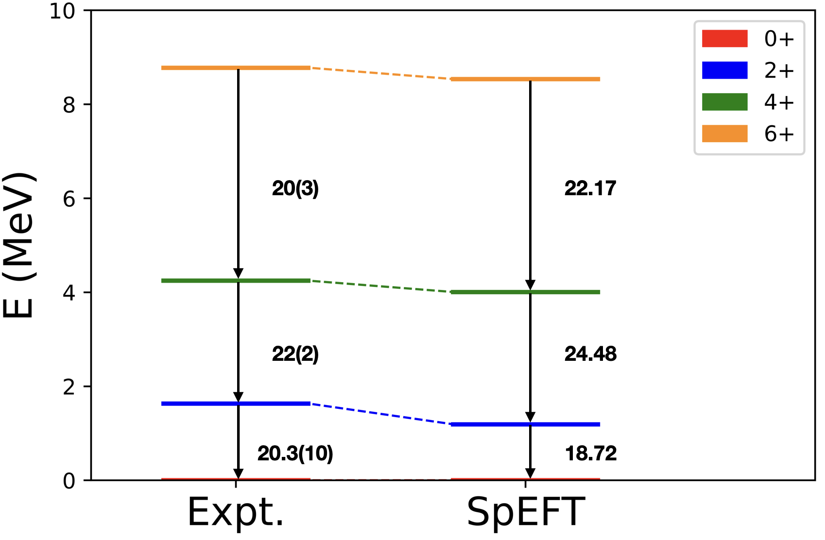
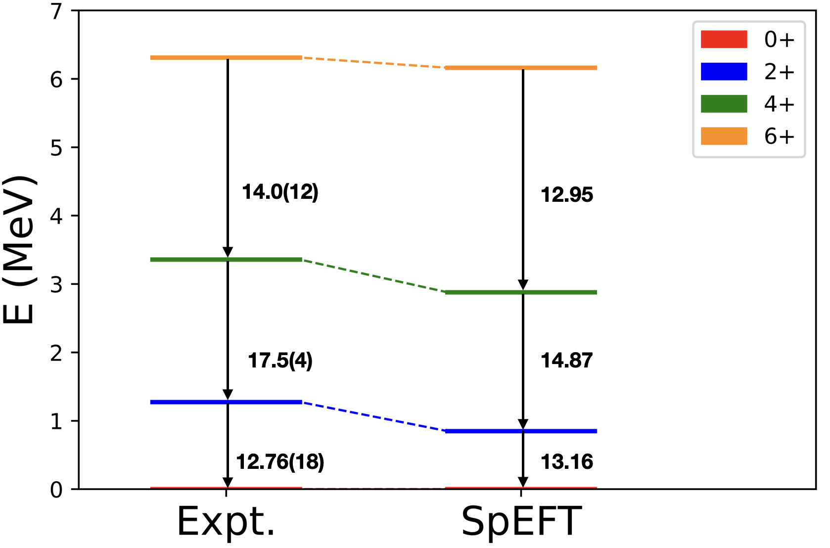
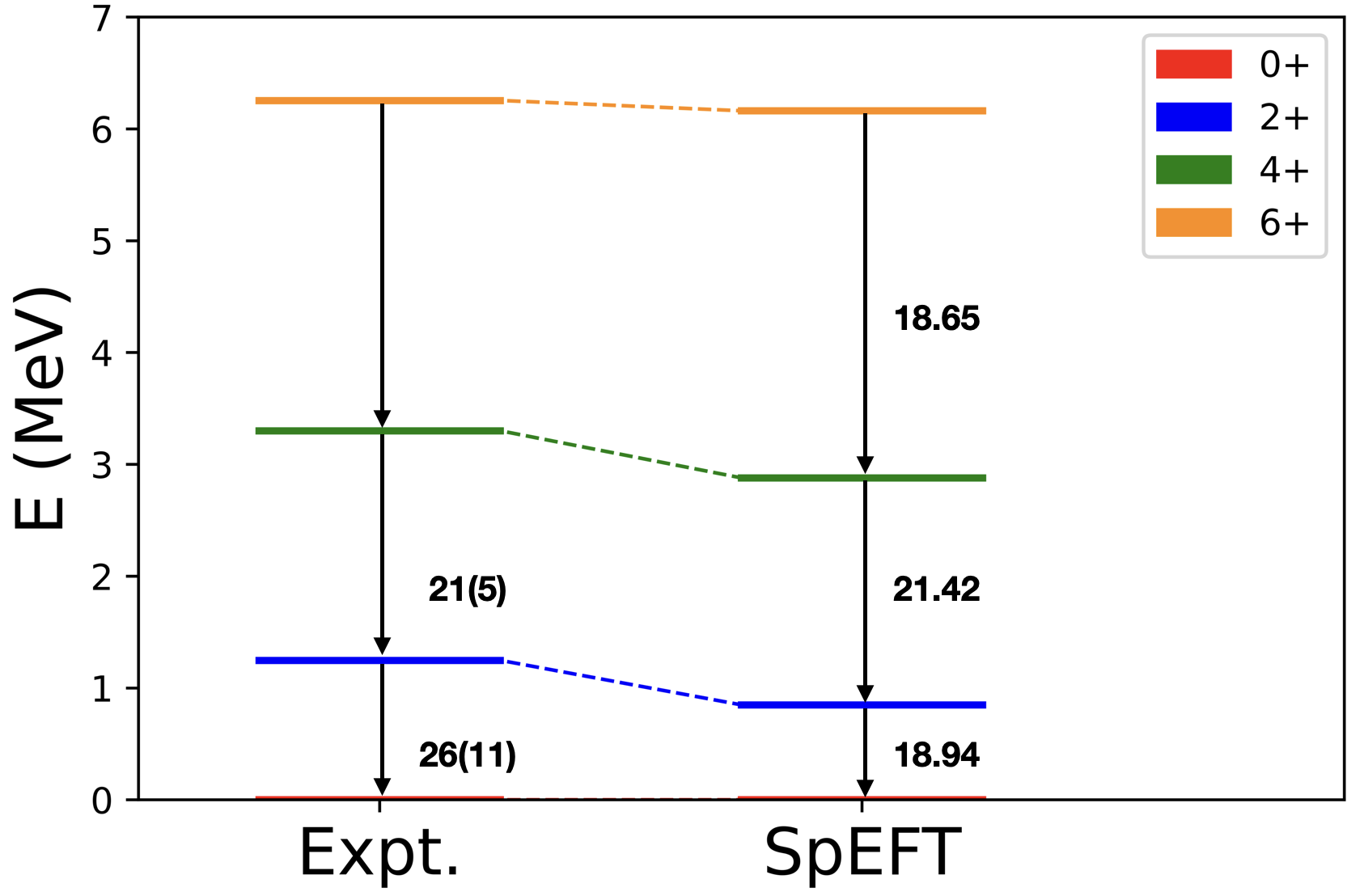
The ground state rotational bands for ²⁰Ne, ²²Ne and ²²Mg all display a structure that is close to that of a rigid rotor, which makes them good tests of our EFT to see if the theory can reproduce this rotational behavior. Moreover, the $K_{ij}K_{ji}$ and $Q_{ij}K_{ji}$ in Eq. (22) should introduce irrotational-like departures from the simple $L(L+1)$ rule for the spectrum of a rigid rotor, which can as well be seen in the ²⁰Ne, ²²Ne, and ²²Mg set, making these ideal candidates for probing a range of rotational features within the context of our EFT theory.

Specifically, we carried out SpEFT calculations in the $N_{\rm{max}}=12$ model space, which was required for gaining good convergence of the observed B(E2) transitions, by adjusting only one parameter; $g=14$ for ²⁰Ne and $g=14.7$ for ²²Ne and ²²Mg. For these nuclei, the $N_{\rm{max}}=12$ model space is down-selected to only one spin-0 leading symplectic irrep; namely $48.5(8,0)$ for ²⁰Ne, $55.5(8,2)$ for ²²Ne and ²²Mg. These selections also proved sufficient to simultaneously reproduce reasonably well-converged values for the observed energy spectra and nuclear radii. And most importantly, the results very clearly demonstrate that the SpEFT is able to do this without the need for introducing effective charges which is confirmed pictorially in Fig. (1,2,3), and by a comparison of the rms radii given in Table (1) that are as well in very good agreement with observations, all with only a single fitting parameter, $g$.

In Table (2) we further give the maximum and minimum values of the scale parameter, $\frac{V_{\mathcal{A}}}{b^{3}N^{3}_{av}}$, for these nuclei. All the presented results are calculated by including terms up to $n\leq 4$ in the Hamiltonian, which, as stressed above, was necessary for gaining good convergence of the theory to known observables. Additionally, we note that for the case of ²⁰Ne, terms with $4<n\leq 6$ contribute $\sim-0.004$ MeV to the ground state energy and $\sim-0.004$ W.u. to the $2^{+}\rightarrow 0^{+}$ B(E2) transition. And beyond these data-focused measures, it is interesting to note that these calculations were all carried out on a laptop, taking from about 10 minutes for the ²⁰Ne case and up to approximately 2 hours for the ²²Ne and ²²Mg cases, a feature which serves to stress that as complex as the underpinning algebraic structure may seem to be (Section II together with the associated Appendices), its applications are computationally quite simple, even to the point of rendering the formalism suitable for more pedagogical uses.

References

- [1] R. Machleidt and D. R. Entem. Chiral effective field theory and nuclear forces. Physics Reports, 503(1):1–75, 2011.
- [2] C. D. Roberts and S. M. Schmidt. Dyson-Schwinger equations: Density, temperature and continuum strong QCD. Progress in Particle and Nuclear Physics, 45:S1–S103, 2000.
- [3] I. C. Cloet and C. D. Roberts. Explanation and prediction of observables using continuum strong QCD. Progress in Particle and Nuclear Physics, 77:1–69, 2014.
- [4] T. Inoue et al. Bound Dibaryon in Flavor Limit of Lattice QCD. Phys. Rev. Lett., 106:162002, Apr 2011.
- [5] M. Mitter, J. M. Pawlowski, and N. Strodthoff. Chiral symmetry breaking in continuum QCD. Phys. Rev. D, 91:054035, Mar 2015.
- [6] G. Eichmann, H. Sanchis-Alepuz, R. Williams, R. Alkofer, and C. S. Fischer. Baryons as relativistic three-quark bound states. Prog. Part. Nucl. Phys., 91:1–100, 2016.
- [7] Steven Weinberg. Effective Field Theory, Past and Future. 2009.
- [8] H. Georgi. An effective field theory for heavy quarks at low energies. Physics Letters B, 240(3):447–450, 1990.
- [9] N. Barnea, L. Contessi, D. Gazit, F. Pederiva, and U. van Kolck. Effective Field Theory for Lattice Nuclei. Phys. Rev. Lett., 114:052501, Feb 2015.
- [10] P. F. Bedaque and U. van Kolck. Effective Field Theory for Few-Nucleon Systems. Annual Review of Nuclear and Particle Science, 52(1):339–396, 2002.
- [11] E. Epelbaum, H.-W. Hammer, and Ulf-G. Meißner. Modern theory of nuclear forces. Rev. Mod. Phys., 81:1773–1825, Dec 2009.
- [12] T. Papenbrock. Effective theory for deformed nuclei. Nuclear Physics A, 852(1):36–60, 2011.
- [13] A. Bohr and B. R. Mottelson. Nuclear Structure, Vol. II: Nuclear Deformation. W. A. Benjamin, Reading, Mas- sachusetts,USA, 1975.
- [14] F. Iachello and A. Arima. The Interacting Boson Model. Cambridge University Press, Cambridge, UK, 1987, 1975.
- [15] S. J. Brodsky et al. Strong QCD from Hadron Structure Experiments: Newport News, VA, USA, November 4-8, 2019. Int. J. Mod. Phys. E, 29(08):2030006, 2020.
- [16] M. Yu. Barabanov et al. Diquark correlations in hadron physics: Origin, impact and evidence. Prog. Part. Nucl. Phys., 116:103835, 2021.
- [17] C. Chen, C. S. Fischer, C. D. Roberts, and J. Segovia. Form Factors of the Nucleon Axial Current. Phys. Lett. B, 815:136150, 2021.
- [18] C. Chen, C. S. Fischer, C. D. Roberts, and J. Segovia. Nucleon axial-vector and pseudoscalar form factors, and PCAC relations. Phys. Rev. D, in press, 2022.
- [19] D. S. Carman, K. Joo, and V. I. Mokeev. Strong QCD Insights from Excited Nucleon Structure Studies with CLAS and CLAS12. Few Body Syst., 61(3):29, 2020.
- [20] V. I. Mokeev and D. S. Carman. Photo- and Electrocouplings of Nucleon Resonances. 2 2022.
- [21] S. Qin and C. D Roberts. Impressions of the Continuum Bound State Problem in QCD. Chin. Phys. Lett., 37(12):121201, 2020.
- [22] C. D. Roberts, D. G. Richards, T. Horn, and L. Chang. Insights into the emergence of mass from studies of pion and kaon structure. Prog. Part. Nucl. Phys., 120:103883, 2021.
- [23] M. G. Mayer and J. H. D. Jensen. Elementary theory of nuclear shell structure. Wiley, 1955.
- [24] J. P. Elliott. Collective motion in the nuclear shell model. I. Classification schemes for states of mixed configurations. Proc. R. Soc. Lond. A, 245:128–145, 1958.
- [25] S. G. Nilsson. Binding states of individual nucleons in strongly deformed nuclei. Kong. Dan. Vid. Sel. Mat. Fys. Med., 29N16:1–69, 1955.
- [26] K. Heyde and J. L. Wood. Shape coexistence in atomic nuclei. Rev. Mod. Phys., 83:1467–1521, Nov 2011.
- [27] G. Rosensteel and D. J. Rowe. Nuclear Model. Phys. Rev. Lett., 38:10–14, Jan 1977.
- [28] D. J. Rowe, G. Thiamova, and J. L. Wood. Implications of Deformation and Shape Coexistence for the Nuclear Shell Model. Phys. Rev. Lett., 97:202501, Nov 2006.
- [29] A. C. Dreyfuss, K. D. Launey, T. Dytrych, J. P. Draayer, and C. Bahri. Hoyle state and rotational features in Carbon-12 within a no-core shell-model framework. Physics Letters B, 727(4):511–515, 2013.
- [30] J. P. Draayer, K. J. Weeks, and G. Rosensteel. Symplectic shell-model calculations for with horizontal configuration mixing. Nuclear Physics A, 413(2):215–222, 1984.
- [31] G. K. Tobin, M. C. Ferriss, K. D. Launey, T. Dytrych, J. P. Draayer, A. C. Dreyfuss, and C. Bahri. Symplectic no-core shell-model approach to intermediate-mass nuclei. Phys. Rev. C, 89:034312, Mar 2014.
- [32] G. Rosensteel, J. P. Draayer, and K. J. Weeks. Symplectic shell-model calculation for . Nuclear Physics A, 419(1):1–12, 1984.
- [33] O. Castaños and J.P. Draayer. Contracted symplectic model with ds-shell applications. Nuclear Physics A, 491(3):349–372, 1989.
- [34] J. Escher and J. P. Draayer. Electron Scattering and Multi- Correlations. Phys. Rev. Lett., 82:5221–5224, Jun 1999.
- [35] C. Bahri and D. J. Rowe. quasi-dynamical symmetry as an organizational mechanism for generating nuclear rotational motions. Nuclear Physics A, 662(1):125–147, 2000.
- [36] O. Castaños, P. O. Hess, J. P. Draayer, and P. Rochford. Pseudo-symplectic model for strongly deformed heavy nuclei. Nuclear Physics A, 524(3):469–478, 1991.
- [37] K. D. Launey, T. Dytrych, and J. P. Draayer. Symmetry-guided large-scale shell-model theory. Progress in Particle and Nuclear Physics, 89:101–136, 2016.
- [38] T. Dytrych, K. D. Sviratcheva, C. Bahri, J. P. Draayer, and J. P. Vary. Evidence for Symplectic Symmetry in Ab Initio No-Core Shell Model Results for Light Nuclei. Phys. Rev. Lett., 98:162503, Apr 2007.
- [39] T. Dytrych, K. D. Launey, J. P. Draayer, P. Maris, J. P. Vary, E. Saule, U. Catalyurek, M. Sosonkina, D. Langr, and M. A. Caprio. Collective Modes in Light Nuclei from First Principles. Phys. Rev. Lett., 111:252501, Dec 2013.
- [40] T. Dytrych, K. D. Launey, J. P. Draayer, D. J. Rowe, J. L. Wood, G. Rosensteel, C. Bahri, D. Langr, and R. B. Baker. Physics of Nuclei: Key Role of an Emergent Symmetry. Phys. Rev. Lett., 124:042501, Jan 2020.
- [41] D. R. Tilley, C. M. Cheves, J. H. Kelley, S. Raman, and H. R. Weller. Energy levels of light nuclei, . Nuclear Physics A, 636(3):249–364, 1998.
- [42] M. S. Basunia. Nuclear Data Sheets for . Nuclear Data Sheets, 127:69–190, 2015.
- [43] L. Chulkov et al. Interaction cross sections and matter radii of isobars. Nuclear Physics A, 603(2):219–237, 1996.
- [44] T. Suzuki et al. Nuclear radii of and isotopes. Nuclear Physics A, 630(3):661–677, 1998.