Symplectically Integrated Symbolic Regression
of Hamiltonian Dynamical Systems
Abstract
Here we present Symplectically Integrated Symbolic Regression (SISR), a novel technique for learning physical governing equations from data. SISR employs a deep symbolic regression approach, using a multi-layer LSTM-RNN with mutation to probabilistically sample Hamiltonian symbolic expressions. Using symplectic neural networks, we develop a model-agnostic approach for extracting meaningful physical priors from the data that can be imposed on-the-fly into the RNN output, limiting its search space. Hamiltonians generated by the RNN are optimized and assessed using a fourth-order symplectic integration scheme; prediction performance is used to train the LSTM-RNN to generate increasingly better functions via a risk-seeking policy gradients approach. Employing these techniques, we extract correct governing equations from oscillator, pendulum, two-body, and three-body gravitational systems with noisy and extremely small datasets.
1 Introduction
Newton, Kepler, and many other physicists are remembered for uncovering mathematical governing equations of complex physical dynamical systems. Ultimately, they were performing exceedingly difficult free-form regression tasks, finding relationships in data sourced from real-world physical observations.
Modern machine learning techniques have demonstrated a broad and impressive ability to extract meaningful relationships from data (Radford et al., 2019; Wang et al., 2017; Krizhevsky et al., 2012). Researchers are increasingly interested in applying such techniques to scientific discovery tasks, particularly in the context of physical dynamical systems and their governing equations (Long et al., 2018, 2019; Qin et al., 2019; Brunton et al., 2020; Raissi & Karniadakis, 2018; Brunton et al., 2016; Tong et al., 2021; Liu & Tegmark, 2021). When compared to traditional machine learning tasks, governing equation discovery offers additional changes in that observation datasets tend to be relatively small and are inevitably tainted with noise or measurement error. Constructing approaches that can learn from a small number of observations while being resistant to noise is a core goal of using machine learning for governing equation discovery. Much of this work has focused on specific formalisms of governing equations, such as Hamiltonians, which provide a consistent approach for many physical dynamical systems and the easy incorporation of priors to shrink the solution space (Greydanus et al., 2019; DiPietro et al., 2020; Chen et al., 2019).
In the past literature, there have been two lines of approaches to learn and predict the time evolution of a physical dynamical system. The first approach emphasizes prediction, relying upon black-box machine learning techniques that can time-evolve the dynamical system with very high accuracy but offer no insight into its underlying governing equations (Greydanus et al., 2019; Chen et al., 2019; Raissi et al., 2020; Breen et al., 2020; Cranmer et al., 2020a). The second approach emphasizes interpretability, prioritizing the discovery of true, concise governing equations for the system (DiPietro et al., 2020; Brunton et al., 2016; Cranmer et al., 2020b; Schmidt & Lipson, 2009; Udrescu & Tegmark, ; Liu & Tegmark, 2021). Interpretable approaches have yielded noteworthy successes, but they often require large amounts of data, fail to learn systems with many degrees of freedom, or require the user to specify function spaces that the governing equation must be contained in. Both black-box and interpretable methods commonly incorporate physics priors, such as symplectic integration schemes, modified loss functions, structure-enforcing formalisms, and constraining equations derived from known physical laws.
In this paper, we present a novel interpretable method: Symplectically Integrated Symbolic Regression (SISR). SISR adopts the Hamiltonian formalism, seeking to uncover governing Hamiltonians of physical dynamical systems solely from position-momenta time series data. First, SISR employs a model-agnostic technique using black-box symplectic networks to extract common Hamiltonian priors, such as coupling, from data. Next, SISR uses the deep symbolic regression paradigm, employing an autoregressive LSTM-RNN that probabilistically generates sequences of function operators, variables, and placeholder constants. These sequences correspond to pre-order traversals of free-form symbolic expressions: in this case, Hamiltonians. The RNN is specially constructed so that only separable Hamiltonian functions are generated. Additionally, the Hamiltonian priors extracted in the initial step are imposed into RNN architecture so that all generated Hamiltonians obey them, drastically reducing the search space. Once generated, these Hamiltonian sequences are translated at run-time into trainable expressions that support auto-differentiation. Each expression has its constants optimized via back-propagation through a symplectic integrator; its prediction performance (reward) is recorded during this process. Then, using a risk-seeking policy gradients approach, the RNN is trained to generate increasingly better symbolic expressions.
Using these techniques, SISR manages to extract correct governing Hamiltonians from four noteworthy dynamical systems, including harmonic oscillator, pendulum, two-body gravitational, and three-body gravitational. All experiments are performed on small training datasets (none them exceed 200 points, as compared to 1000+ in other state-of-the-art approaches), with and without Gaussian noise. To our knowledge, SISR is the first free-form, interpretable machine learning approach that can discover governing Hamiltonians of systems with many degrees of freedom using small-scale, noisy data samples.
In summary, we propose SISR, a novel technique for extracting governing Hamiltonians from observation data, which makes the following key architectural contributions:
-
1.
Employs a model-agnostic approach using symplectic neural networks to extract common Hamiltonian priors from data.
-
2.
Uses a specially constructed LSTM-RNN with mutation to generate separable Hamiltonians that obey the extracted Hamiltonian priors.
-
3.
Imposes a further symplectic prior on the RNN-generated expressions by training their constants via backpropagation through a symplectic integrator.
2 Related Work
Symbolic Regression: Traditional and Deep
Often, regression techniques parameterize underlying functions using specific functional forms, such as lines or polynomials. Symbolic regression, on the other hand, performs its regression search over the space of all mathematical functions that can be constructed from some given set of operators: the form is essentially arbitrary. Traditionally, symbolic regression has relied upon genetic programming techniques (O’Neill, 2009; Lu et al., 2016; Cranmer et al., 2020b). Recently, researchers have begun incorporating modern deep learning approaches. Sahoo et al. (2018) parameterize spaces of symbolic functions using neural networks with specially constructed activation functions. More recently, Petersen et al. (2019) introduce the deep symbolic regression model, which uses an autoregressive RNN to generate symbolic expressions and then trains it using a novel policy-gradients approach. Mundhenk et al. (2021) augment the deep symbolic regression approach, using an RNN-guided symbolic expression search to construct populations for use with genetic programming. Note that most of these techniques are for the general symbolic regression task, lacking any priors unique to physical dynamical systems.
Computational Techniques for Governing Equation Discovery
There has been considerable research done on machine learning models that can extract mathematically concise governing functions from physical systems. Brunton et al. (2016) propose SINDy, which operates within a pre-specified function space (i.e. polynomial, trigonometric, etc.) and performs a L1-regularized sparse regression, learning which terms to keep. DiPietro et al. (2020) introduce SSINNs, which use a similar approach to SINDy but frame the problem using the Hamiltonian formalism and perform the sparse optimization by back-propagating through a symplectic integrator, which incorporates a symplectic bias into the symbolic expressions. These sparse approaches are limited in that the governing function must exist in the pre-specified function space in order to be found. Cranmer et al. (2020b) use graph neural networks, representing particles as nodes and forces between pairs of particles as edges. After training these graph models, they extract symbolic expressions by using Eureqa to fit the edge, node, and global models of their graph networks. However, their experiments involve a relatively large volume of clean data. Schmidt & Lipson (2009) employ a genetic, free-form symbolic regression approach that focuses upon conserved quantities such as Lagrangians and Hamiltonians; they succeed in learning governing equations for systems such as the double pendulum. Finally, there are numerous other approaches for equation discovery that follow different paradigms altogether (Long et al., 2018, 2019; Raissi & Karniadakis, 2018; Saemundsson et al., 2020; Sun et al., 2019).
Symplectic Machine Learning Models
In recent years, many works have incorporated symplectomorphism as a physics prior; as a result, they tend to use the Hamiltonian formalism as well. Greydanus et al. (2019) propose Hamiltonian Neural Networks, which parameterize Hamiltonians using black-box deep neural networks. They optimize the gradients of these networks via back-propagation through a leapfrog numerical integrator, which gives rise to conserved quantities in the model. Chen et al. (2019) employ a similar approach but opt for a symplectic integrator and recurrent neural network; they achieve noteworthy prediction results but, due to their choice of integrator, can only learn separable Hamiltonians. Xiong et al. (2020) provide a novel architecture that incorporates symplectic priors but is not limited to separable Hamiltonians; they achieve noteworthy results on both separable and non-separable systems, including chaotic vortical flows. DiPietro et al. (2020), mentioned above, use a symplectic prior to augment an interpretable sparse regression approach. Symplectic priors are used by a variety of other works as well (Tong et al., 2021; Zhu et al., 2020; Mattheakis et al., 2019; Jin et al., 2020).
3 Background
SISR learns governing equations in the Hamiltonian formalism and employs a model-agnostic approach to extract Hamiltonian coupling priors. Here we offer mathematical background on Hamiltonian mechanics and coupling.
3.1 Hamiltonian Mechanics
Hamiltonian mechanics is a reformulation of classical mechanics introduced in 1833 by William Rowland Hamilton. The Hamiltonian formalism provides a consistent approach for mathematically describing a variety of physical dynamical systems; it is heavily used in quantum mechanics and statistical mechanics, often for systems with many degrees of freedom (Morin, 2008; Reichl, 2016; Taylor, 2005; Sakurai & Napolitano, 2010; Hand & Finch, 1998).
In Hamiltonian mechanics, dynamical systems are governed via their Hamiltonian , a function of the momenta and position vectors ( and respectively) of each object in the system. The value of the Hamiltonian generally measures the total energy of the system; for systems where energy is conserved, is time-invariant. Further, we say that is separable if it can be decomposed into two additively separable functions and , where measures kinetic energy and measures potential energy.
The time evolution of a physical dynamical system is uniquely defined by the partial derivatives of its Hamiltonian:
| (1) |
The time evolution of a Hamiltonian system is symplectomorphic, preserving the symplectic two-form . As a result, researchers generally time-evolve Hamiltonians with symplectic integrators, which are designed to preserve this two-form. We employ a fourth-order symplectic integrator (pseudocode in Appendix A) (Forest & Ruth, 1990).
3.2 Coupling
Hamiltonians commonly exhibit coupling: they can be written as a series of additively separable functions where each function takes some smaller subset of variables. Consider some arbitrary n-body, m-dimensional separable Hamiltonian where the bodies are labeled and the dimensions are labeled . What coupling might occur?
Without loss of generality, consider . Denote the momentum of body in dimension as . We say that exhibits complete decoupling if it may be rewritten as the sum of functions that each take only one variable in the system, i.e. it may be written in the form:
| (2) |
We say that exhibits dimensional coupling if it may be rewritten as the sum of functions that each take all dimensional variables for only a single particle in the system, i.e. it may be written in the form:
| (3) |
Finally, we say that exhibits pairwise coupling if it may be rewritten as the sum of functions that each take all dimensional variables for a pair of particles in the system, i.e. where denotes all momenta variables of particle , may be written in the form:
| (4) |
3.3 Coupling Composite Functions
Consider some arbitrary coupling function . Often, may be written as a composition of functions where performs one of several common reduction operations, such as summing, multiplication, Euclidean distance, or Manhattan distance. In these instances, we would say that particles are coupled via the given inner operation, such as their sum. If is known, then one may learn by learning , which tends to be much simpler than learning the entire directly.
3.4 Symmetries
Suppose that a Hamiltonian function exhibits pairwise coupling, i.e., it may be written as the sum of many additively separable coupling functions. Often, across all pairs of particles, these coupling functions are identical (symmetric). For instance, in an n-body gravitational system with particles of equal mass, or an n-body electrostatic system with particles of equal charge, all particles are pairwise coupled using the exact same coupling function.
4 Algorithm
Here we present the SISR architecture, which consists of a coupling extraction process followed by a deep symbolic regression-inspired training loop. This training loop can further be decomposed into expression generation (4.2), symplectic optimization (4.3), and RNN training (4.4).
4.1 Extracting Function Properties via Symplectic Neural Networks
As detailed in Sections 3.2, 3.3, and 3.4, Hamiltonians commonly exhibit coupling properties. These properties may be used to simplify the Hamiltonian discovery process by imposing restrictions that dramatically reduce the solution space. Thus, the first step of SISR is to find what coupling is taking place in the Hamiltonian, whether it can be reduced into simpler composite functions, and whether it is symmetric across particles or pairs of particles.
Our approach for doing this is rooted in symplectic neural networks as effective black-box predictors of Hamiltonian dynamical systems. Specifically, we can construct multi-layer neural networks that enforce specific coupling properties. Then, we may train these networks by using them to time-evolve the dynamical system through a symplectic integrator. By seeing how these networks perform with and without imposed coupling properties, we may deduce whether those properties hold for the system. To the best of our knowledge, we are the first work to extract coupling properties in the context of Hamiltonian dynamical systems, and we are not aware of any other work that employs symplectic neural networks in a similar manner.
4.1.1 Coupling
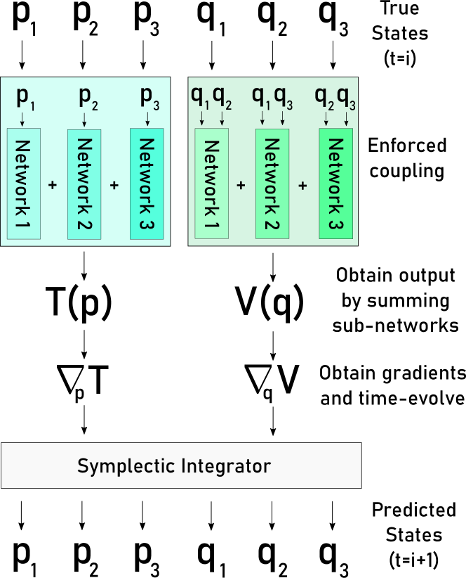
In order to assess whether a physical dynamical system exhibits a particular variety of coupling, we can construct a model that enforces one of the functional forms described in Equations 2, 3, or 4. We do this by parameterizing the individual coupling functions with neural networks and summing the individual outputs of these networks to get the entire function output for or . Note that these models are trained via gradient descent through a symplectic integrator; this process is depicted for a 3-body pairwise-momentum dimensional-position model in Figure 1.
Although this method works for assessing specific instances of coupling, the question still remains of how we construct a search over and , as the couplings of these functions are independent. Additionally, even if a Hamiltonian exhibits pairwise coupling, it doesn’t mean that all particles in the system are necessarily pairwise coupled. Our search approach is simple and works well empirically.
We begin by training a model where and are each parameterized by a single network, meaning that there are no coupling properties enforced. The value of the performance metric for this model is used to set a baseline. Then, holding this network constant for , we enforce complete decoupling in . If the corresponding performance metric drop is above some pre-defined fixed percentage relative to the baseline, denoted the maximum tolerable performance decrease, we say that the is in fact completely decoupled. Otherwise, we attempt dimensional coupling and possibly pairwise coupling. This process is then repeated for , with the network in held constant. Note that, if pairwise coupling is found, we perform a recursive backwards elimination to see which pairs must be present; this elimination process requires an additional maximum tolerable performance decrease parameter; this parameter is generally smaller, as it is easy to overfit to pairs that aren’t actually present in the Hamiltonian, especially with little data.
4.1.2 Coupling Composite Functions
Once coupling has been identified, we determine whether the quantities are coupled by their sum, product, distance, or some other operation. To do this, we modify the network so that the operation being tested is performed immediately on the input variables prior to the forward pass. Then, we select the best performing composite function that meets the maximum tolerable performance decrease.
4.1.3 Symmetries
Once we have determined which particles are coupled and by what, if any, composite functions, we assess whether the coupling functions are symmetric across all pairs of particles. To do this, we use the same neural network for all coupled quantities (such as all pairs of positions in an n-body gravitational system). Note that this requires that the domain of input values for each particle are reasonably close. If the performance doesn’t degrade below our tolerance, we say that the couplings are symmetric.
4.2 Generating Symbolic Hamiltonians
With our coupling properties determined, we are ready to begin generating candidate symbolic Hamiltonians. We do this via a deep symbolic regression approach, employing an LSTM-RNN.
First, note that free-form symbolic functions may be represented as trees where internal nodes are functional operators and leaves are variables or constants. The pre-order traversal of this expression tree produces a sequence that uniquely defines the symbolic expression. Thus, sequence-generating RNNs can be used in an autoregressive manner to produce symbolic functions. We refer to functional operators, variables, and constants as tokens in the sequence.
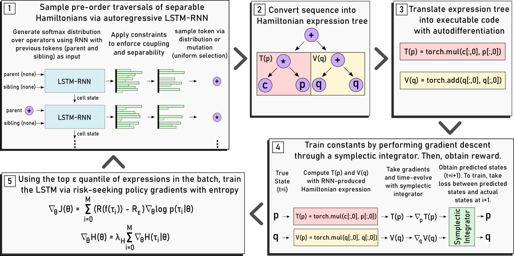
To generate a symbolic expression, an LSTM-RNN generates a sequence from left-to-right. As input, the network takes a one-hot encoding of the parent and sibling token for the current token being sampled. It then emits a softmax distribution, which is adjusted to eliminate all invalid tokens. This distribution may be sampled to generate the next token in the sequence. We also employ an epsilon-greedy mutation approach where the next token is sampled uniformly from the list of valid tokens with probability, where is a pre-defined hyperparameter. This process is depicted in Step 1 of Figure 2.
Due to our use of a fourth-order symplectic integrator, we require that any Hamiltonian generated by the LSTM-RNN is of the form . This constraint is applied in situ, meaning that the softmax distribution over the operators is constantly adjusted as expressions are generated so that only Hamiltonians of this form will ever be produced. This same approach is used to incorporate any coupling properties previously discovered: the emitted distribution is adjusted prior to sampling a token so that we will only ever see Hamiltonians that exhibit the desired coupling. To the best of our knowledge, this is the first instance of an LSTM-RNN being used to generate separable Hamiltonians with desired coupling properties.
Once a Hamiltonian sequence is generated, it is translated into an executable model with auto-differentiation (Steps 2 and 3 of Figure 2). The first reason for this is to that constants can be optimized–the sequence contains placeholder “ephemeral” constants that do not refer to specific values. The second purpose is so that the performance of the expression can be assessed. This is done by numerically integrating the Hamiltonian to predict the system, which requires the ability to take its gradients.
4.3 Symplectic Optimization
As mentioned previously, candidate Hamiltonian functions must have their placeholder constants trained. This is performed via a symplectic optimization approach (Step 4 of Figure 2). Using a fourth-order symplectic integrator and a time-series of observation data for the system, we use the candidate Hamiltonian to time-evolve the system and obtain predicted future states. We then take the loss between our predicted future states and the actual future states contained in the observation data, backpropagating through our integrator to train the constants and thus imparting an energy-conserving symplectic prior onto any Hamiltonian generated by the RNN. This approach, which has been applied to black-box system prediction methods with great success, has yet to be employed for any free-form symbolic regression model (Chen et al., 2019; DiPietro et al., 2020).
4.4 Training the RNN
Thus far, we have presented an RNN that can generate separable Hamiltonians (with specific coupling properties) that are then trained via backpropagation through a symplectic integrator. However, in order for a symbolic Hamiltonian search to succeed, the RNN must be trained to produce progressively better-fitting Hamiltonians.
To do this, we employ the risk-seeking policy gradients approach presented by Petersen et al. (2019), which maximizes the best-case expectation of rewards for expressions generated by the policy (in this case the RNN). To do this, we train on the top quantile in some given batch, where is referred to as the risk factor. First, let this quantile consist of expressions where denotes the -th expression in the quantile. If defines a symplectic integration function, defines a reward function, defines the reward of the top quantile, and defines the expectation of rewards in the top quantile conditioned on the weights of the RNN, we have:
| (5) |
In the event that the expression generation involved mutation, we compute using the probabilities produced by the RNN–not the uniform probabilities generated to sample the mutated operator.
Further, as in Petersen et al. (2019), we adopt the maximum entropy framework and include an entropy term in the loss (Haarnoja et al., 2018). Where is the entropy coefficient, we have:
| (6) |
Note that refers to the Shannon entropy function and is not a Hamiltonian.
This training process corresponds to Step 5 of Figure 2. We are not aware of any other approach for Hamiltonian dynamical systems that employs these reinforcement learning-oriented training approaches.
5 Experiments
We assess SISR by applying it to four noteworthy Hamiltonian dynamical systems: the harmonic oscillator, the pendulum, the two-body gravitational system (the Kepler problem), and the three-body gravitational system. Aside from expression length, all experiments use the same set of hyperparameters, which are almost entirely replicated from Petersen et al. (2019) and detailed in Appendix B.1.
For each experiment, we generated 3 different time series datasets via fourth-order symplectic integration with different initial conditions, which are available in Appendix B.2. These datasets are exceedingly small–smaller than any other work in this domain that we are aware of. Each experiment was conducted a total of 5 times on each dataset. Note that each dataset consists entirely of training data, as either SISR extracts the correct governing Hamiltonian from the training data or it does not. We say that a SISR-generated Hamiltonian is correct if it is algebraically equivalent to the true Hamiltonian with precision in its constants. Our LSTM-RNN was optimized with Adam and employed an NRMSE reward function.
In initial experiments, we noticed very high variance in the number of epochs needed to obtain the Hamiltonian. We believe that this may be a consequence of the initial batch being too small to adequately explore the function space. As a result, we set the initial batch size to times the regular batch size; we adjust the risk factor to compensate, meaning that the RNN is trained on the same number of expressions after each batch.
5.1 Harmonic Oscillator
The harmonic oscillator is a one-dimensional, single-particle dynamical system described by the Hamiltonian
| (7) |
where is the mass of the particle and refers to its oscillator frequency.
We trained SISR on 3 different datasets of harmonic oscillator motion with varying initial conditions, each consisting of only points from to . In addition to variables and constants, SISR had access to the operators . The and of each generated Hamiltonian were limited to be between and operators long. SISR was applied to each dataset 5 times, recovering the correct Hamiltonian for all 15 trials. This took an average of batches, or seconds. In 4 out of 15 instances, the Hamiltonian was uncovered after a single epoch. Next, we applied SISR to the same datasets with of Gaussian noise. Once again, it uncovered the correct Hamiltonian in all trials, requiring an average of batches, or seconds.
5.2 Pendulum
The pendulum is an angular, single-particle dynamical system described by the Hamiltonian
| (8) |
where is mass, is gravity, and is length.
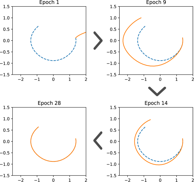
Using the functional operators , we trained SISR on 3 different datasets of pendulum motion with varying initial conditions, containing points from to . The and of each generated Hamiltonian were limited to be between and operators long. With no noise present, SISR recovered the correct Hamiltonian in all 15 trials, taking an average of batches, or seconds. When of Gaussian noise was added to each dataset, SISR recovered all correct Hamiltonians in batches, or seconds. Hamiltonians generated by SISR for the pendulum problem are depicted in Figure 3.
5.3 Two-Body Gravitational System
The two-body gravitational system is a two-dimensional dynamical system described by the Hamiltonian
| (9) |
with mass for particles and . Note that we work explicitly with two-body systems where all masses are equal and .
We began by extracting coupling properties via the symplectic neural network procedures described in Section 4.1. Using this process, we first determined that particle positions were pairwise coupled, as well as that particle momenta were completely decoupled. Then, we were able to decompose the position coupling into a composite function of Euclidean distance. Finally, we determined that the functions acting on the momenta of each particle are symmetric. The exact numerical results used to guide this search process are available in Appendix B.3. Once these coupling constraints are imposed on the RNN, the solution space shrinks dramatically. Rather than learning and outright as in our previous experiments, we are effectively learning the pairwise position coupling function between particles, which is itself a function of their Euclidean distance, and the decoupled momentum function acting on each particle.
Using the functional operators , we trained SISR on 3 different datasets of two-body motion with varying initial conditions, containing points from to . The and of each generated Hamiltonian were limited to be between and operators long. With no noise present, SISR recovered the correct Hamiltonian for all 15 trials, taking an average of batches, or seconds. When of Gaussian noise was added to each dataset, SISR recovered all correct Hamiltonians in batches, or seconds. Note how powerful our extracted coupling priors are: with them imposed, the two-body Hamiltonian is learned more quickly than a pendulum Hamiltonian.
| NRMSE | Extracted Correct Equation | ||||||||
|---|---|---|---|---|---|---|---|---|---|
| Problem | SISR | SINDy | SSINN | DSR | SISR | SINDy | SSINN | DSR | |
| Harm. Osc. (Clean) | |||||||||
| Harm. Osc. (Noisy) | |||||||||
| Pendulum (Clean) | |||||||||
| Pendulum (Noisy) | |||||||||
| Two-Body (Clean) | |||||||||
| Two-Body (Noisy) | |||||||||
| Three-Body (Clean) | |||||||||
| Three-Body (Noisy) | |||||||||
5.4 Three-Body Gravitational System
The three-body gravitational system is a two-dimensional dynamical system described by the Hamiltonian
| (10) |
with mass for particles , , and . This system exhibits chaotic motion, meaning that small perturbations in initial conditions diverge exponentially in the future (Sprott, 2010).
We followed a nearly identical coupling extraction process to our two-body experiments, identifying that all particles are pairwise coupled as a function of their Euclidean distance, as well as all momenta being completely decoupled and symmetric. These results are detailed in Appendix B.3.
Using the functional operators , we trained SISR on 3 different datasets of three-body motion with points each. The and of each generated Hamiltonian were limited to be between and operators long. Five trials were conducted on each dataset. With no noise present, SISR took an average of epochs, or seconds, to recover the Hamiltonian (all were recovered). With of Gaussian noise present, SISR required an average of epochs, or seconds (all were recovered).
5.5 Comparison to Existing Techniques
We benchmarked SISR against two other methods for obtaining physical governing equations for data: SINDy and SSINNs. Both of these methods rely upon sparse regressions in user-defined function spaces. They obtained reasonable NRMSE for many problems but only extracted correct governing equations in 2 of 8 instances. Indeed, with so little data, it is easy for sparse-regression oriented methods to overfit to excess terms. Finally, we compared to the vanilla deep symbolic regression model, which we used to generate systems of differential equations instead of Hamiltonians. These results are summarized in Table 1 with further experimental details available in Appendix B.4.
6 Scope and Limitations
Limited to separable Hamiltonians
SISR uncovers the dynamics of physical systems by generating separable Hamiltonians, but not all physical dynamical systems can be represented in this way. Real-world systems often exhibit energy dissipation that can violate our formalism. Being robust to such dissipation, or knowing when to switch formalisms, may serve as a basis for future work.
Coupling extraction complexity
Our coupling extraction process requires training a large number of black-box symplectic neural networks. Unfortunately, as the physical dynamics of a system become increasingly complicated, these networks must increase in size to maintain predictive accuracy. In doing so, they become more time-consuming to train and further risk overfitting to the system.
Computationally expensive constant optimization
Every expression generated by the LSTM-RNN must have its constants optimized. This means that, over the course of the entire Hamiltonian generation process, many thousands of expressions will need to be optimized. Empirically, this operation accounts for approximately 96% of the run-time for SISR. Many of these expressions do not fall in the top quantile, meaning that they are not used to trained the RNN. We leave optimizations to this process for future work.
7 Conclusion
Here we present Symplectically Integrated Symbolic Regression, a new technique for extracting governing Hamiltonians from time series observations of a physical dynamical system. By applying a model-agnostic coupling extraction approach, we are able to generate priors that greatly benefit our model, allowing it to quickly fit oscillator, pendulum, 2-body and 3-body systems from no more than 200 noisy observations. These results are state-of-the-art in their performance and simultaneous use of small data. Future work may include methods for extracting additional Hamiltonian priors besides coupling, as well as modifications that allow for energy dissipation.
References
- Breen et al. (2020) Breen, P. G., Foley, C. N., Boekhold, T., and Zwart, S. P. Newton versus the machine: solving the chaotic three-body problem using deep neural networks. Monthly Notices of the Royal Astronomical Society, 494(2):2465–2470, 2020.
- Brunton et al. (2020) Brunton, S., Noack, B., and Koumoutsakos, P. Machine learning for fluid mechanics, 2020. https://arxiv.org/abs/1905.11075.
- Brunton et al. (2016) Brunton, S. L., Proctor, J. L., and Kutz, J. N. Discovering governing equations from data by sparse identification of nonlinear dynamical systems. PNAS, 113(15):3932–3937, 2016.
- Chen et al. (2019) Chen, Z., Zhang, J., Arjovsky, M., and Bottou, L. Symplectic recurrent neural networks, 2019. https://arxiv.org/abs/1909.13334.
- Cranmer et al. (2020a) Cranmer, M., Greydanus, S., Hoyer, S., Battaglia, P., Spergel, D., and Ho, S. Lagrangian neural networks. arXiv preprint arXiv:2003.04630, 2020a.
- Cranmer et al. (2020b) Cranmer, M., Sanchez-Gonzalez, A., Battaglia, P., Xu, R., Cranmer, K., Spergel, D., and Ho, S. Discovering Symbolic Models from Deep Learning with Inductive Biases. 2020b.
- DiPietro et al. (2020) DiPietro, D. M., Xiong, S., and Zhu, B. Sparse symplectically integrated neural networks. In Advances in Neural Information Processing Systems 33, pp. 6074–6085. 2020.
- Forest & Ruth (1990) Forest, E. and Ruth, R. D. Fourth-order symplectic integration. Physica D: Nonlinear Phenomena, 43(1):105–117, 1990.
- Greydanus et al. (2019) Greydanus, S., Dzamba, M., and Yosinski, J. Hamiltonian neural networks. In Advances in Neural Information Processing Systems 32, pp. 15379–15389. 2019.
- Haarnoja et al. (2018) Haarnoja, T., Zhou, A., Abbeel, P., and Levine, S. Soft actor-critic: Off-policy maximum entropy deep reinforcement learning with a stochastic actor. In International conference on machine learning, pp. 1861–1870. PMLR, 2018.
- Hand & Finch (1998) Hand, L. N. and Finch, J. D. Analytical Mechanics. Cambridge University Press, Cambridge, England, 1998.
- Jin et al. (2020) Jin, P., Zhang, Z., Zhu, A., Tang, Y., and Karniadakis, G. E. Sympnets: Intrinsic structure-preserving symplectic networks for identifying hamiltonian systems. Neural Networks, 132:166–179, 2020.
- Krizhevsky et al. (2012) Krizhevsky, A., Sutskever, I., and Hinton, G. E. Imagenet classification with deep convolutional neural networks. In Advances in Neural Information Processing Systems 25, pp. 1097–1105. 2012.
- Liu & Tegmark (2021) Liu, Z. and Tegmark, M. Machine learning conservation laws from trajectories. Physical Review Letters, 126(18):180604, 2021.
- Long et al. (2018) Long, Z., Lu, Y., Ma, X., and Dong, B. PDE-net: Learning PDEs from data. In Proceedings of the 35th International Conference on Machine Learning, pp. 3208–3216, 2018.
- Long et al. (2019) Long, Z., Lu, Y., and Dong, B. Pde-net 2.0: Learning pdes from data with a numeric-symbolic hybrid deep network. Journal of Computational Physics, 399:108925, 2019.
- Lu et al. (2016) Lu, Q., Ren, J., and Wang, Z. Using genetic programming with prior formula knowledge to solve symbolic regression problem. Computational intelligence and neuroscience, 2016, 2016.
- Mattheakis et al. (2019) Mattheakis, M., Protopapas, P., Sondak, D., Di Giovanni, M., and Kaxiras, E. Physical symmetries embedded in neural networks. arXiv preprint arXiv:1904.08991, 2019.
- Morin (2008) Morin, D. J. Introduction to Classical Mechanics: With Problems and Solutions. Cambridge University Press, Cambridge, England, 2008.
- Mundhenk et al. (2021) Mundhenk, T., Landajuela, M., Glatt, R., Santiago, C., Petersen, B., et al. Symbolic regression via deep reinforcement learning enhanced genetic programming seeding. Advances in Neural Information Processing Systems, 34, 2021.
- O’Neill (2009) O’Neill, M. Riccardo poli, william b. langdon, nicholas f. mcphee: a field guide to genetic programming, 2009.
- Petersen et al. (2019) Petersen, B. K., Larma, M. L., Mundhenk, T. N., Santiago, C. P., Kim, S. K., and Kim, J. T. Deep symbolic regression: Recovering mathematical expressions from data via risk-seeking policy gradients. arXiv preprint arXiv:1912.04871, 2019.
- Qin et al. (2019) Qin, T., Wu, K., and Xiu, D. Data driven governing equations approximation using deep neural networks. Journal of Computational Physics, 395:620–635, 2019.
- Radford et al. (2019) Radford, A., Wu, J., Child, R., Luan, D., Amodei, D., and Sutskever, I. Language models are unsupervised multitask learners. 2019.
- Raissi & Karniadakis (2018) Raissi, M. and Karniadakis, G. E. Hidden physics models: Machine learning of nonlinear partial differential equations. Journal of Computational Physics, 357:125–141, 2018.
- Raissi et al. (2020) Raissi, M., Yazdani, A., and Karniadakis, G. E. Hidden fluid mechanics: Learning velocity and pressure fields from flow visualizations. Science, 367(6481):1026–1030, 2020.
- Reichl (2016) Reichl, L. E. A Modern Course in Statistical Physics. Wiley-VCH, Weinheim, Germany, 2016.
- Saemundsson et al. (2020) Saemundsson, S., Terenin, A., Hofmann, K., and Deisenroth, M. P. Variational integrator networks for physically structured embeddings, 2020.
- Sahoo et al. (2018) Sahoo, S., Lampert, C., and Martius, G. Learning equations for extrapolation and control. In International Conference on Machine Learning, pp. 4442–4450. PMLR, 2018.
- Sakurai & Napolitano (2010) Sakurai, J. J. and Napolitano, J. J. Modern Quantum Mechanics (2nd Edition). Pearson, London, England, 2010.
- Schmidt & Lipson (2009) Schmidt, M. and Lipson, H. Distilling free-form natural laws from experimental data. Science, 324(5923):81–85, 2009.
- Sprott (2010) Sprott, J. C. Elegant Chaos: Algebraically Simple Flows. World Scientific, Singapore, 2010.
- Sun et al. (2019) Sun, Y., Zhang, L., and Schaeffer, H. Neupde: Neural network based ordinary and partial differential equations for modeling time-dependent data, 2019.
- Taylor (2005) Taylor, J. R. Classical Mechanics. University Science Books, Mill Valley, California, 2005.
- Tong et al. (2021) Tong, Y., Xiong, S., He, X., Pan, G., and Zhu, B. Symplectic neural networks in taylor series form for hamiltonian systems. Journal of Computational Physics, 437:110325, 2021.
- (36) Udrescu, S.-M. and Tegmark, M. Ai feynman: A physics-inspired method for symbolic regression. Science Advances, 6(16).
- Wang et al. (2017) Wang, F., Jiang, M., Qian, C., Yang, S., Li, C., Zhang, H., Wang, X., and Tang, X. Residual attention network for image classification. In Proceedings of the IEEE Conference on Computer Vision and Pattern Recognition, pp. 3156–3164, 2017.
- Xiong et al. (2020) Xiong, S., Tong, Y., He, X., Yang, S., Yang, C., and Zhu, B. Nonseparable symplectic neural networks. arXiv preprint arXiv:2010.12636, 2020.
- Zhu et al. (2020) Zhu, A., Jin, P., and Tang, Y. Deep hamiltonian networks based on symplectic integrators. arXiv preprint arXiv:2004.13830, 2020.
Appendix A Symplectic Integration Pseudocode
We employ the fourth-order symplectic integrator introduced by (Forest & Ruth, 1990), defined in Algorithm 1.
This algorithm employs the constants , , , , and .
Appendix B Extended Experimental Details
B.1 SISR Hyperparameter Selection
All experiments used the same set of SISR hyperparameters, aside from their expression lengths and functional operators. These hyperparameters were largely obtained from (Petersen et al., 2019), with the exception of mutation rate, number of layers, initial batch size, inner learning rate, inner optimizer, and inner number of epochs. These additional hyperparameters worked well with their initially selected values and did not require any tuning.
All SISR models were trained with a learning rate , entropy coefficient , mutation rate , risk factor , batch size of 500, and initial batch size of 2000. The RNN architecture was a two-layer LSTM with 250 nodes per layer and initial state optimization. It was optimized using Adam. Expressions generated by the RNN were trained for 15 epochs with a learning rate of ; they were optimized using RMSProp.
B.2 Initial Conditions
Each experiment used three datasets with different sets of initial conditions. These initial conditions are detailed in Tables 2, 3, 4, and 5.
| Dataset | ||||
|---|---|---|---|---|
| 1 | 1.23 | 1.65 | -0.05 | 0.42 |
| 2 | 0.63 | 1.30 | 0.27 | -0.29 |
| 3 | 1.69 | 0.83 | 0.06 | -0.54 |
| Dataset | |||||
|---|---|---|---|---|---|
| 1 | 0.47 | 1.23 | 1.95 | 1.32 | 0.23 |
| 2 | 1.10 | 0.73 | 1.02 | 1.37 | 0.12 |
| 3 | 0.68 | 0.33 | 1.59 | 0.87 | 0.15 |
| Dataset | ||||||
|---|---|---|---|---|---|---|
| 1 | 1 | 1 | (0.00, 0.00) | (1.00, 1.00) | (0.00, 1.00) | (1.00, 0.00) |
| 2 | 1 | 1 | (0.00, 0.00) | (0.50, 1.00) | (0.34, 0.30) | (1.00, 0.21) |
| 3 | 1 | 1 | (0.00, 0.50) | (0.30, -0.24) | (0.40, -1.00) | (-0.80, -2.10) |
| Dataset | |||||||||
|---|---|---|---|---|---|---|---|---|---|
| 1 | 1 | 1 | 1 | (0.00, 0.00) | (1.00, 1.00) | (-1.00, -1.00) | (0.50, 0.30) | (1.10, -0.40) | (-0.20, 0.50) |
| 2 | 1 | 1 | 1 | (0.00, 0.00) | (-3.00, 0.00) | (3.00, 0.00) | (0.00, -1.00) | (0.50, 0.00) | (0.50, 0.00) |
| 3 | 1 | 1 | 1 | (0.25, 0.25) | (2.00, 1.50) | (3.00, -2.00) | (0.00, -1.00) | (0.50, -0.15) | (0.80, 0.25) |
B.3 Extracting Function Properties via Symplectic Neural Networks
Using the technique described in Section 4.1, we extracted coupling properties for our two-body and three-body experiments. Both systems used the same symplectic network architecture: each block was 8 hidden layers deep with 128 hidden neurons per layer. We used GeLU as our activation function and trained for 3,000 epochs via Adam with a learning rate of . This architecture was largely inspired by the successful three-body prediction network in Breen et al. (2020), with some slight hand-adjustments made to hyperparameters. In order to reduce overfitting, we trained the network for 10 steps of prediction at a time. To do this, the dataset of 200 points was broken into a set of 180 for training and a set of 10 for testing, such that the set of 10 for testing has no overlap with a 10-step prediction made from any training point. The batch size was set to the entire set of 180 training points.
B.3.1 Two-Body Results
Using the architecture described in B.3, we began our experiments by attempting to determine the coupling present in the system. We set our maximum tolerable performance decrease to 10%. Using this approach, our technique correctly deduced for both our clean and noisy datasets that exhibits pairwise coupling whereas exhibits complete decoupling; these results are contained in Tables 6 and 7. With these results determined, we began the next search for pairwise position composite functions, again with a maximum tolerable performance decrease of 10%. This tolerance was met by both Manhattan distance and Euclidean distance composite functions. However, Euclidean distance outperformed Manhattan distance, so it was selected as the composite function. These results are depicted for our clean and noisy datasets in Tables 8 and 9. Finally, we assessed whether the completely decoupled momenta functions are symmetric across all quantities; enforcing this symmetry increased performance in both our clean and noisy datasets (Tables 10 and Table11). Thus, we were able to determine that the exhibits pairwise coupling as a function of Euclidean distance and that exhibits complete decoupling with symmetric subfunctions for all quantities.
B.3.2 Three-Body Results
Our three-body coupling search preceded similarly to the our two-body search, correctly identifying that exhibits pairwise coupling as a function of Euclidean distance and that exhibits complete decoupling with symmetric subfunctions. For this search, however, the tolerable decline was set to 5%. Additionally, since there are 3 pairs of particles, we performed a recursive backwards elimination with a tolerance of 1% to see which pairs were necessary–it was determined that all were. Coupling results are contained in Tables 12 and 13 and coupling composite results are contained in Tables 14 and 15.
B.4 Comparison Details
We compared our method to SINDy, SSINNs, and Vanilla Deep Symbolic Regression. Here we provide some further context on the hyperparameters used for each of these methods.
For SINDy, we employed the standard function library for all tasks except for the pendulum, where we added Fourier terms. The regularization parameter was initially set to . As SINDy cannot directly learn Hamiltonians, we instead learned a system of differential equations. If all coefficients were removed for any of the given differential equations, we decreased the regularization parameter in increments of so that this did not happen. If the equations became too long to numerically integrate within seconds, we raised the regularization parameter in increments of so that this did not happen. We planned on converting these differential equations to Hamiltonians so that we could time-evolve with a symplectic integrator. However, many of the systems of differential equations were not separable, so we instead unrolled their predictions using RK4.
For SSINNs, we employed the 3rd degree polynomial function library for all tasks except for the pendulum, where we added a shiftable sine term. We used the hyperparameters described in DiPietro et al. (2020), setting a learning rate of with decay and a regularization term of . We trained this architecture for 100 epochs.
Finally, we employed vanilla Deep Symbolic Regression. Although not well-suited for physical dynamical systems, we modified this model to produce a series of differential equations, similar to SINDy. Again, these differential equations did not necessarily convert to a separable Hamiltonian, so we trained the model by numerically integrating them with RK4 to obtain a reward. We employed the same architecture and hyperparameters defined by Petersen et al. (2019), using a 250-node RNN with 0.0005 learning rate, 0.95 risk factor, 0.005 entropy coefficient, and 500 batch size. Then, we trained the model for 200 epochs and optimized with Adam. These hyperparameters worked quite well, as the model achieved reasonable performance for not having any physical priors imposed.
B.5 Hardware Information
All SISR models were trained on an Intel i7-9750H CPU, which was found to be comparable in training time to using GPU. Symplectic Neural Networks were trained on an NVIDIA GeForce GTX 1650 GPU.
| NRMSE | Performance Change | ||
|---|---|---|---|
| No coupling enforced (baseline) | No coupling enforced (baseline) | N/A (baseline) | |
| Complete decoupling enforced | No coupling enforced | ||
| Dimensional coupling enforced | No coupling enforced | ||
| Pairwise coupling enforced | No coupling enforced | N/A (baseline) | |
| Pairwise coupling enforced | Complete decoupling enforced |
| Composite Function Enforced | NRMSE | Performance Change |
|---|---|---|
| None (baseline) | N/A (baseline) | |
| Sum | ||
| Product | ||
| Manhattan Distance | ||
| Euclidean Distance |
| Composite Function Enforced | NRMSE | Performance Change |
|---|---|---|
| None (baseline) | N/A (baseline) | |
| Sum | ||
| Product | ||
| Manhattan Distance | ||
| Euclidean Distance |
| Symmetry Enforced | NRMSE | Performance Change |
|---|---|---|
| None (baseline) | N/A (baseline) | |
| Complete symmetry |
| Symmetry Enforced | NRMSE | Performance Change |
|---|---|---|
| None (baseline) | N/A (baseline) | |
| Complete symmetry |
| NRMSE | Performance Change | ||
|---|---|---|---|
| No coupling enforced (baseline) | No coupling enforced (baseline) | N/A (baseline) | |
| Complete decoupling enforced | No coupling enforced | ||
| Dimensional coupling enforced | No coupling enforced | ||
| Pairwise coupling enforced | No coupling enforced | ||
| Pairwise coupling (i,j and j,k) | No coupling enforced | ||
| Pairwise coupling (i,j and i,k) | No coupling enforced | ||
| Pairwise coupling (i,k and j,k) | No coupling enforced | ||
| Pairwise coupling enforced | Complete decoupling enforced |
| Composite Function Enforced | NRMSE | Performance Change |
|---|---|---|
| None (baseline) | N/A (baseline) | |
| Sum | ||
| Product | ||
| Manhattan Distance | ||
| Euclidean Distance |
| Composite Function Enforced | NRMSE | Performance Change |
|---|---|---|
| None (baseline) | N/A (baseline) | |
| Sum | ||
| Product | ||
| Manhattan Distance | ||
| Euclidean Distance |