Synergistic Learning with Multi-Task DeepONet for Efficient PDE Problem Solving
Abstract
Multi-task learning (MTL) is an inductive transfer mechanism designed to leverage useful information from multiple tasks to improve generalization performance compared to single-task learning. It has been extensively explored in traditional machine learning to address issues such as data sparsity and overfitting in neural networks. In this work, we apply MTL to problems in science and engineering governed by partial differential equations (PDEs). However, implementing MTL in this context is complex, as it requires task-specific modifications to accommodate various scenarios representing different physical processes. To this end, we present a multi-task deep operator network (MT-DeepONet) to learn solutions across various functional forms of source terms in a PDE and multiple geometries in a single concurrent training session. We introduce modifications in the branch network of the vanilla DeepONet to account for various functional forms of a parameterized coefficient in a PDE. Additionally, we handle parameterized geometries by introducing a binary mask in the branch network and incorporating it into the loss term to improve convergence and generalization to new geometry tasks. Our approach is demonstrated on three benchmark problems: (1) learning different functional forms of the source term in the Fisher equation; (2) learning multiple geometries in a 2D Darcy Flow problem and showcasing better transfer learning capabilities to new geometries; and (3) learning 3D parameterized geometries for a heat transfer problem and demonstrate the ability to predict on new but similar geometries. Our MT-DeepONet framework offers a novel approach to solving PDE problems in engineering and science under a unified umbrella based on synergistic learning that reduces the overall training cost for neural operators.
keywords:
multi-task learning , neural operators , DeepONet , scientific machine learning1 Introduction
In scientific machine learning, we can solve partial differential equations (PDEs) by finding the solution operator, known as the neural operator (NO). The NO takes different functions as inputs, such as initial and boundary conditions, and maps them to the solution of the PDE. Traditional numerical methods such as finite difference, finite element, and spectral methods are generally used to compute solutions to PDEs. There is an increasing interest in using scientific machine learning methods to solve PDEs in real time across diverse applications. However, these real-time methods can be computationally expensive when dealing with high dimensional PDEs, and incorporating experimental measurement data as model inputs is often not possible. Additionally, the solution must be recomputed for minor changes in the input function or the geometry domain that add to the computational burden for the users.
Recently, Deep neural networks (DNNs) have been employed in NOs [1, 2] to approximate mappings between infinite-dimensional Banach spaces, in contrast to the finite-dimensional vector space mapping learned through functional regression in conventional DNNs. Frameworks such as deep operator network (DeepONet) [3] and integral operators, which include architectures like the Fourier neural operator (FNO) [4], the wavelet neural operator (WNO) [5], the Laplace neural operator (LNO) [6], and convolutional neural operator (CNO) [7], have demonstrated significant potential over a range of applications. While the early success of NOs has been promising, their predictive performance is often limited by the availability of labeled data for training. Collecting large labeled datasets for each task can be computationally intractable, especially for high-fidelity or multi-scale models. Multi-task learning (MTL) is an alternative mechanism aimed at leveraging useful information from related learning tasks to address data sparsity and overfitting issues [8]. This inductive transfer mechanism trains tasks in parallel while using a shared representation, assuming that the tasks are associated with each other and that shared information among them can lead to synergistic learning performance.
MTL has been explored in traditional machine learning tasks such as natural language processing, computer vision, and healthcare to improve generalization scenarios with limited training data. There are two prevalent techniques for using MTL based on the connections between the learning tasks: hard parameter sharing and soft parameter sharing. Hard parameter sharing uses a common hidden layer for all tasks, while soft parameter sharing regularizes the distance between parameters in different models. Hard parameter sharing techniques are useful when tasks have different input data distributions but similar output conditional distributions (i.e., and ), typically referred to as covariate shift. MTL has received significant attention in the domain of computer vision. Some notable works include Liu et al.’s [9] deep fusion with LSTM modules, and Long et al.’s [10] joint adaptation networks for transfer learning. In the computer vision, MTL methods such as PAD-Net [11], MTAN [12], and cross-stitch networks [13] have achieved significant advancements in tasks such as depth estimation, scene parsing, and surface normal prediction. Recently, Reed et al. [14] introduced GATO, a generalist agent using the transformer architecture to handle multiple tasks like image captioning, gaming, playing Atari, etc. simultaneously, demonstrating remarkable versatility. Liu [15] introduced an in-context learning paradigm to learn a common operator mapping from a set of differential equations. Liu et al. utilize a transformer framework where key-value pairs are used as input queries for predicting the output solution of a differential equation. The key-value pair represents conditions that define the differential equation such as the initial condition in a temporal problem. This framework shows good generalization capabilities due to its in-context learning paradigm.
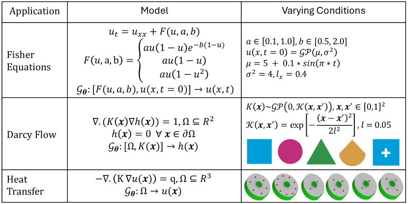
Liu’s research presents a good opportunity for developing multi-task operator frameworks that can be applied to realistic problems, particularly in engineering and life sciences. One significant challenge for the operator network relates to handling varying geometric domains, a problem that is not addressed in current frameworks including Liu’s. In science and engineering tasks, the application of MTL frameworks is complicated, since PDEs with the same initial or boundary conditions can represent vastly different physical systems. However, a group of tasks can share the same marginal distribution of inputs or even the same input function, while their conditional output distributions may differ significantly. This scenario, known as conditional shift, occurs when and . In such cases, transfer learning, often referred to as soft parameter sharing, has shown success. In our recent study [16], we proposed the idea of transfer learning within the DeepONet (TL-DeepONet) architecture to enable the knowledge transfer from one task to a related but different task, allowing task-specific learning under conditional shift. However, we found limitations in this framework when attempting to transfer knowledge across varying geometries, such as changes in internal and external boundaries of the target geometry. In this work, we aim to extend DeepONet’s capability to train multiple parameterized PDEs on multiple domains concurrently, enhancing the generalizability of a single network and thereby improving the transfer learning process to new geometric domains. To achieve this, we introduce multi-task DeepONet (MT-DeepONet) designed to predict solutions for different but correlated tasks in a single training session. Figure 1 illustrates the problem statements for the MTL problems considered in this study of MT-DeepONet. The main contributions of this work are summarized as follows:
-
•
Extension of DeepONet for concurrent training over multiple tasks: We develop MT-DeepONet to approximate the solution for multiple tasks (different parametric conditions and source terms) simultaneously, without requiring re-training.
-
•
Improved generalizability: We investigate the generalization ability of MT-DeepONet for knowledge sharing across different geometries as an extension to [16]. We demonstrate improvement in target model learning across varied geometries using the MTL source model as compared to a single-task source model.
-
•
Enhanced knowledge transfer: We introduce a masking operation that enables our MT-DeepONet to learn solutions across varied geometries. Our methodology is demonstrated by learning solutions for D Darcy flow equations across multiple geometric domains and steady-state heat transfer in multiple D plate designs parameterized by the location and number of heating sources.
The paper is organized as follows. In Section 2, we provide a brief review of the original DeepONet framework followed by a description of the proposed MT-DeepONet framework. In Section 3, we present a comprehensive collection of problems for which the proposed MT-DeepONet has been extensively studied. We discuss the data generation process and include results and comparisons for multiple examples. Finally, we summarize our observations and provide concluding remarks in Section 4 along with some limitations of the framework.
2 Multi-task learning in neural operators
Neural operators learn nonlinear mappings between functional spaces on bounded domains, offering a unique framework for real-time solution inference for complex parametric PDEs. Here, ‘parametric PDEs’ refer to PDE systems with parameters that vary over a certain range. Typically, DeepONet (our choice of operator network for this work) is trained on a fixed domain, , for varying parametric conditions drawn from a distribution. In this work, we introduce MT-DeepONet, which enables concurrent training of multiple functions (leading to different dynamics) and multiple geometries, along with varying parametric conditions. This section provides a brief overview of the DeepONet architecture and extends it to discuss our multi-task DeepONet framework.
2.1 Deep operator network
The goal of operator learning is to learn a mapping between two infinite-dimensional spaces on a bounded open set , given a finite number of input-output pairs. Let and be Banach spaces of vector-valued functions defined as:
| (1) | |||
| (2) |
where and denote the set of input functions and the corresponding output functions, respectively. The operator learning task is defined as . The objective is to approximate the nonlinear operator, , via the following parametric mapping:
| (3) |
where is a finite-dimensional parameter space. In the standard setting, the optimal parameters are learned by training the neural operator with a set of labeled observations , which contains pairs of input and output functions. When a physical system is described by PDEs, it involves multiple functions, such as the PDE solution, the forcing term, the initial condition, and the boundary conditions. We are typically interested in predicting one of these functions, which is the output of the solution operator (defined on the space ), based on the varied forms of the other functions, i.e., the input functions in the space .
The deep operator network (DeepONet) is inspired by the universal approximation theorem for operators [17]. The architecture of DeepONet comprises two deep neural networks: the branch network and the trunk network. The branch network encodes the input functions at fixed sensor points , while the trunk network encodes the information related to the spatio-temporal coordinates where the solution operator is evaluated. The trunk network takes these spatial and temporal coordinates to compute the loss function. The solution operator for an input realization can be expressed as:
| (4) |
where are the output embeddings of the branch network and are the output embeddings of the trunk network. In Eq. (4), represents the trainable parameters of the network including weights, , and biases, . The optimized parameters , are obtained by minimizing a standard loss function ( or ) using a standard optimization algorithm.
The DeepONet model provides a flexible framework that allows the branch and trunk networks to be configured with different architectures. For equispaced discretization of the input function, a convolutional neural network (CNN) can be utilized for the branch network architecture, whereas a multilayer perceptron (MLP) is often employed for a sparse representation of the input function. An MLP is commonly used for the trunk network to handle the low-dimensional evaluation points, . Since its inception, standard DeepONet has been applied to address complex, high-dimensional systems [18, 19, 20, 21, 22, 23, 24]. Recent extensions for DeepONet have explored multi-fidelity learning [25, 26, 27], integration of multiple-input continuous operators [28, 29], hybrid transferable numerical solvers [30, 31], resolution independent learning [32], transfer learning [33], physics-informed learning to satisfy the underlying PDE [34, 2, 35], and learning in latent spaces [36].
2.2 Multi-task deep operator network (MT-DeepONet)
Neural operators are inherently data-driven models that require substantial datasets to develop a generalized solution operator for parameterized PDEs. In general, applications using DeepONet to learn the solution operator have focused on single-domain geometries, parameterizing either the source term or the initial condition with a Gaussian random field. In this work, our goal is to develop a generalized solution operator capable of accommodating various functional forms of source terms and their parameterization, across multiple geometries. The different applications explored in this study are illustrated in Figure 1. The MT-DeepONet framework is designed to:
-
•
Learn multiple source terms representing different physical systems in a single training process, demonstrated through the Fisher equation.
-
•
Simultaneously learn the solution operator on different geometries, thereby improving the source model’s ability to transfer knowledge to a target model. This is illustrated by solving the Darcy flow problem in various D geometries and learning the temperature distribution across multiple unique D engineering geometries.
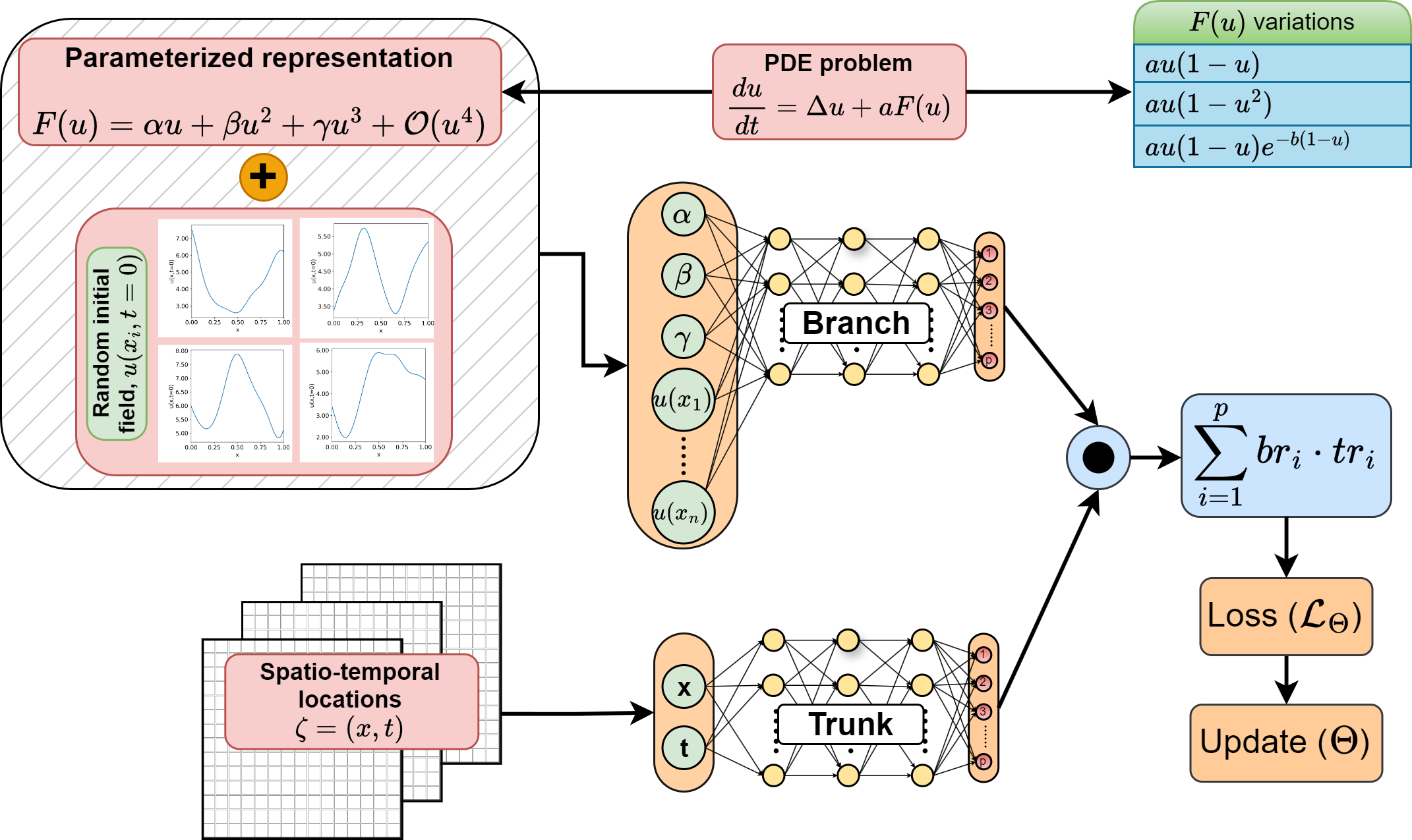
The primary modification in the MT-DeepONet framework occurs in the branch network of the standard DeepONet architecture. Each problem is addressed uniquely. For example, in the case of multiple source terms in the Fisher equation (see Figure 1), the source terms are represented as a polynomial to create a unique representation for each equation:
| (5) |
The coefficients of the dependent variable in this polynomial expression are used as inputs to the branch network, along with the random initial conditions that define the problem. A schematic of the framework is shown in Figure 2 for understanding. Further details of the problem are discussed in Section 3.1.
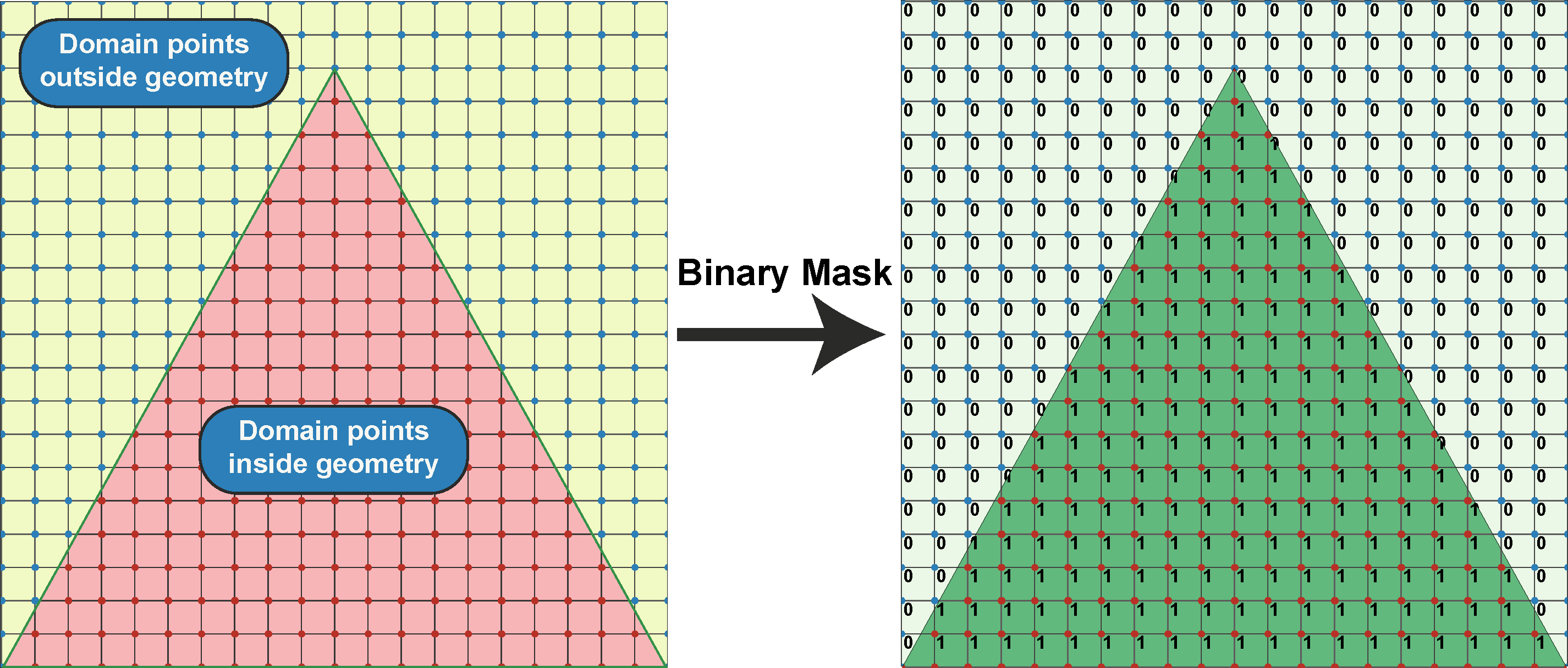
To accommodate varying geometries concurrently in a single training process, we use a binary mask (array of ’s and ’s). This mask is constructed by fitting the geometry within a unit square plate for D problems and a box for D problems. The masking function assigns a value of to points within the boundary of the desired geometry and to points outside the boundary but within the plate or box. Figure 3 illustrates the masking function with a triangular geometry within a square plate. The solution operator is defined as the product of (as described in Equation 4) and the binary masking function, ensuring the solution is confined within the geometry’s bounds. Algorithm 1 details the steps for training the MT-DeepONet with a binary mask to address problems across multiple geometries. This approach also tests our hypothesis that learning multiple geometries improves the source model’s ability to transfer knowledge to target models with different geometries (Section 3.2). However, given the complexity of such knowledge transfer in the diverse range of PDEs representing different physical systems, we demonstrate the effectiveness of the masking framework for learning the solution operator across unseen 3D geometries in a steady-state heat transfer problem (Section 3.3).
MTL serves as an inductive transfer mechanism designed to enhance generalization performance compared to single-task learning. It achieves this by leveraging valuable information from multiple learning tasks and utilizing domain-specific insights embedded within training samples across related tasks. In our study, we demonstrate the effectiveness of MTL in learning solutions across diverse sets of PDEs, initial conditions, and geometries simultaneously.
3 Numerical examples
In this section, we explore the capabilities of the proposed MT-DeepONet framework on three problems shown in Figure 1. Detailed information on data generation for each problem can be found in Supplementary S1, while specifics about the network architecture are provided in Supplementary S3.
3.1 Fisher Equations
The first example considers the Fisher equation proposed by Ronald Fisher in , which provides a mathematical framework for analyzing population dynamics and chemical wave propagation with diffusion [37]. The original reaction-diffusion equation is defined as:
| (6) |
where represents population density that varies spatially and temporally, and are scalar parameters denoting the diffusion coefficient and the intrinsic growth rate, respectively. In dimensionless form, this equation is written as:
| (7) |
Kolmogorov, Petrovsky, and Piskunov introduced a more general form, the Fisher-KPP equation [38]:
| (8) |
where the population density, , varies along two spatial dimensions , and the reaction term must satisfy the following criteria:
| (9a) | |||
| (9b) | |||
| (9c) | |||
| (9d) | |||
Assuming that the density is invariant along the -axis, the Fisher-KPP equation in dimensionless form is re-written as:
| (10) |
| Equation |
|
|
|
||||||
|---|---|---|---|---|---|---|---|---|---|
| Fisher [37] | |||||||||
| Newell–Whitehead–Segel [40] | |||||||||
| Zeldovich–Frank–Kamenetskii [41] |
|
In the conventional operator learning task, the focus is typically on analyzing the change in density profile over a one-dimensional spatiotemporal domain and for parameterized initial condition drawn from a distribution. Due to diffusion, regions with higher density expand over time towards areas with lower density, based on the initial distribution. For our MT-DeepONet, we aim to evaluate the Fisher-KPP model to learn the density variation over time for two tasks: () varying initial conditions of density , and (ii) three reaction functions in a single training cycle, considering different functional of that are separately parameterized by two scalar coefficients and . We generate multiple initial conditions as a Gaussian random field and multiple forcing functions using the Fisher-KPP general form with three reaction terms from the literature, as listed in Table 1.
To incorporate the different functional forms of as inputs to the network, we express the functions as shown in Equation 5. For the Zeldovich form, we use the Taylor expansion and re-write it as:
| (11) |
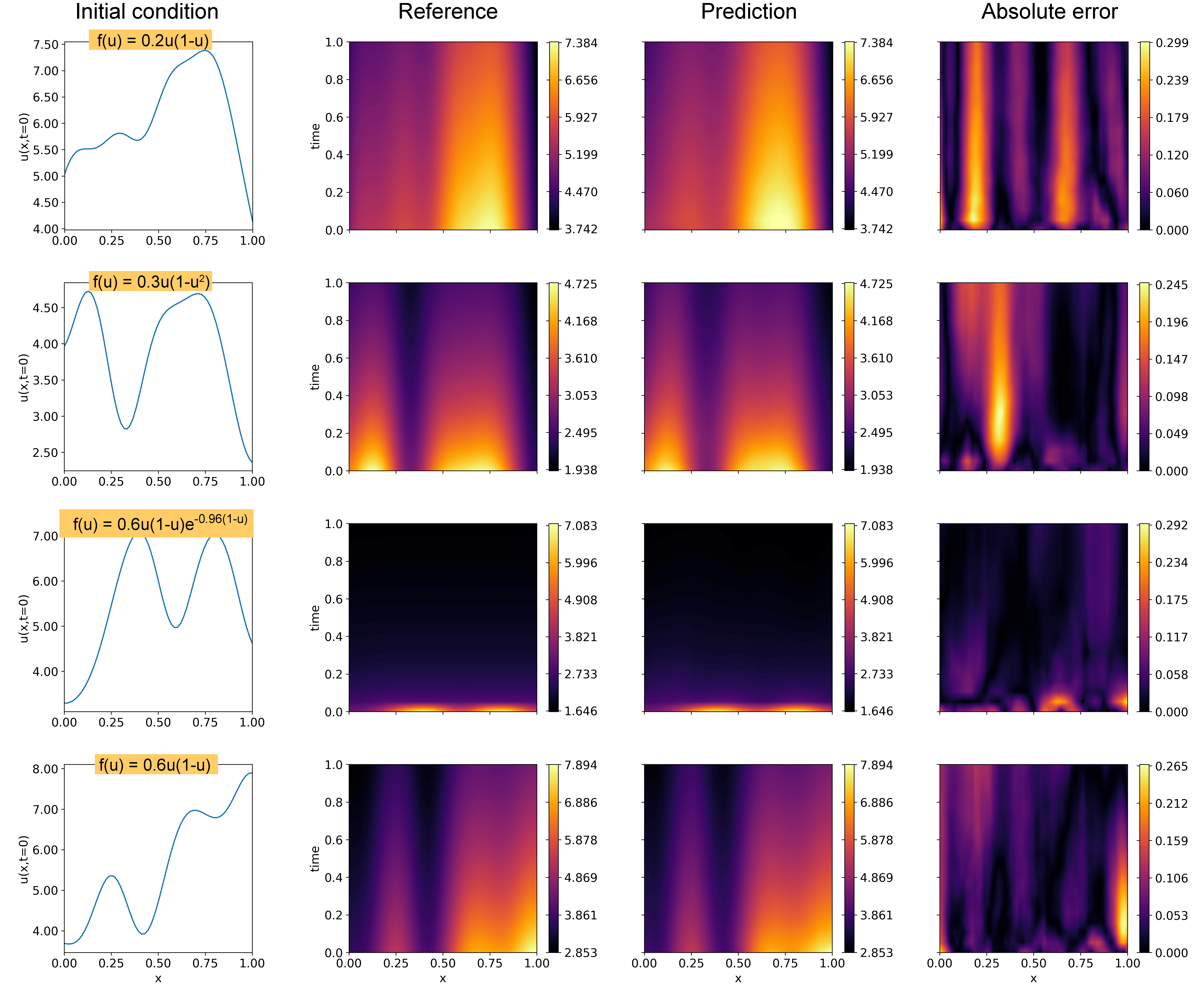
The coefficients of , , and are represented as , and , respectively in Figure 2, with the constant term is denoted as . To train the MT-DeepONet for the Fisher-KPP equations, the coefficients of the parameterized form of are concatenated with the flattened initial conditions, and used as inputs to the branch network. We use Adam optimizer with a progressively reducing learning rate and the network is trained for , epochs using mean-squared error as the loss function. The relative norm for the test samples is approximately . Figure 4 presents four representative test case predictions using the MT-DeepONet. The results indicate that the multi-task operator network can capture large-scale features across the space-time domain with reasonable accuracy, under varying initial conditions and parameters of the Fisher-KPP equation. Additionally, the training time for individual DeepONet for each forcing term with varying initial conditions was - seconds on an NVIDIA A100 GPU. In contrast, the MT-DeepONet framework was trained in seconds, showing the computational effectiveness of our approach.
3.2 Darcy Flow in D geometries
In the second example, we consider the Darcy flow through a bounded domain and aim to train multiple D geometries (bounded domains) simultaneously considering parameterized spatially varying conductivity fields. An earlier attempt, as noted in [42], focused on learning similar yet parameterized geometries in a concurrent training session. In contrast, our work demonstrates the learning of distinctly different geometries.
Darcy’s law describes fluid flow through a porous medium, relating pressure, velocity, and medium permeability. The pressure in the porous medium is expressed as [20]:
| (12) | ||||
| (13) |
where denotes spatially varying hydraulic conductivity field, is the hydraulic head, and is the source term. For simplicity, we set . The objectives for multi-task operator learning to predict the hydraulic head, , include () spatially varying conductivity fields drawn from a Gaussian random field, and () operation on varying D geometries. In this task, we aim to demonstrate the generalization ability of MT-DeepONet through transfer learning, where the target domains differ geometrically from the source domains. The source and target geometries considered in this example are shown in Figure 5. The source geometries are labeled with S, while the target geometries are labeled with T. The source MT-DeepONet involves training on source domains S concurrently with sufficient labeled data, which is later transferred to related target domains T where only a small amount of training data is available. To capture geometric variation in a single training session, the conductivity field is combined with a binary mask and used as input to the branch network, which employs a CNN architecture. The trunk network receives inputs from a uniformly discretized square domain , subdivided into a uniform grid. For all geometries, ground truth data is obtained using the MATLAB PDE Toolbox on an irregular mesh and thereafter interpolating the solution onto this regular grid. The trunk network’s basis functions (output embeddings) are used to evaluate the solution field at all domain points. The solution field outside the domain boundary is enforced to be zero by multiplying the solution operator with the binary mask. This mask ensures the solution is zero outside the geometry, thus improving convergence. Refer to Algorithm 1 showing the implementation details of this workflow.


Transfer learning across different geometries
In this section, we investigate how multi-task training in the source model enhances generalization across different geometries in target models. To assess the effectiveness of transfer learning, we train four source models using various geometric combinations: S1, S1+S2, S1+S3, and S1+S2+S3. Each source model is trained on a total of 5,400 samples. For single-geometry models (e.g., S1), all samples are from the same geometry. For multi-geometry models, we evenly distribute samples across the geometries: 2,700 samples from each geometry for S1+S2 and S1+S3, and 1,800 samples from each geometry for S1+S2+S3. We train the MT-DeepONet using a piece-wise constant learning rate scheduler with rates [0.001, 0.0005, 0.0001] over 5,000 epochs, employing mini-batching with a batch size of and optimizing with mean squared error. This experimental setup allows us to evaluate how the diversity of geometries in the source model affects the transfer learning process and subsequent performance on target models. Figure 6 presents three representative cases of predicted solutions when source MT-DeepONet was trained concurrently with geometries S + S + S. The binary mask is applied to the output of the operator network to enforce that solutions outside the geometric domain are zero. The results demonstrate that the source MT-DeepONet has accurately learned all three geometries. Table 2 presents the relative errors for various source model configurations. We observe a trend of increasing error as the number of geometries in the training data grows. This pattern is consistent with our expectations, given the multi-task feature set that the operator network must learn during multi-geometry training. While this approach may lead to a slight reduction in accuracy for individual tasks, it offers a more versatile representation across multiple geometries. This trade-off between task-specific performance and cross-geometry generalization is a key aspect of our multi-task learning strategy.
We employ transfer learning to adapt our trained source multi-task operator network for new geometries T1 and T2. The target models are considered distinct tasks. The transfer learning process begins by initializing the network with trained parameters from the source model. The layers updated during fine-tuning include the first input CNN layer of the branch network, three MLP layers following the convolution modules in the branch, and the linear output layer of the trunk network. We assess the prediction accuracy of the target model using varying numbers of training samples from the target domain: 50, 100, 200, 500, and 800. This approach significantly reduces computational costs for learning pressure heads on new geometries. Table 2 presents a summary of errors obtained from the target models for different test cases. Our analysis reveals distinct error patterns for target geometries T1 and T2. For T1, the source model combination S1 + S2 yields a lower error compared to the single-geometry S1 source model. This demonstrates that training on multiple geometries can enhance the network’s transfer learning capabilities. Conversely, source models with geometrical combinations S1 + S3 and S1 + S2 + S3 result in higher errors in the target model compared to single-task learning on geometry S1. These findings underscore a crucial insight: naively combining all source tasks does not universally improve prediction performance for the target task. This phenomenon, known as negative transfer, occurs when source tasks unrelated to the target tasks are included. In our case, the results indicate that source geometry S3 introduces a negative transfer effect. Negative interference is a known challenge in MTL and we plan to explore mitigation strategies in future research. Conversely, for geometry T2, the source model S1 yields similar error values to the combination S1 + S2, indicating no significant improvement with the multi-task source model. This result may be attributed to the similarity between geometry T2 and S1. Figures 7 and 8 compare predictions from the transfer learning model against reference solutions for different source models trained with samples used to fine-tune the target model. The source model was trained with samples where each geometry had equal representation.
| Source geometry model | Source model rel error | Target geometry |
|
||||||
|---|---|---|---|---|---|---|---|---|---|
| n = 50 | n = 100 | n = 200 | n = 500 | n = 800 | |||||
| S1 | 0.029 | T1 | 0.082 | 0.063 | 0.055 | 0.047 | 0.045 | ||
| S1+S2 | 0.039 | T1 | 0.065 | 0.054 | 0.048 | 0.047 | 0.044 | ||
| S1+S3 | 0.061 | T1 | 0.088 | 0.080 | 0.070 | 0.064 | 0.061 | ||
| S1+S2+S3 | 0.054 | T1 | 0.083 | 0.068 | 0.060 | 0.055 | 0.054 | ||
| S1 | 0.029 | T2 | 0.158 | 0.132 | 0.106 | 0.083 | 0.077 | ||
| S1+S2 | 0.039 | T2 | 0.163 | 0.137 | 0.105 | 0.085 | 0.080 | ||
| S1+S3 | 0.061 | T2 | 0.152 | 0.134 | 0.117 | 0.102 | 0.098 | ||
| S1+S2+S3 | 0.054 | T2 | 0.158 | 0.138 | 0.119 | 0.098 | 0.094 | ||
Transfer learning in the context of disparate geometric domain, T3
Our next objective is to investigate whether incorporating multiple geometries in the source model helps reduce the prediction error when transferring to target geometries with different external boundaries. To further explore the efficacy of multi-geometry training in transfer learning, we introduce an I-section geometry (T3) as our target for transfer learning. Our hypothesis posits that a source model trained on multiple geometries simultaneously can more effectively transfer knowledge to a new target domain. To validate this hypothesis, we compare the prediction errors of transfer learning models derived from single-geometry source models against the one trained on multiple geometries. Table 3 outlines the source geometry combinations employed in this study: S3, S5, S7, and the multi-geometry combination S3-S7. For consistency, each source model was trained on a total of 5,400 samples. The results, also presented in Table 3, reveal that the lowest prediction error for target geometry T3 is achieved when the source model is trained on multiple geometries simultaneously. Notably, the improvement in prediction accuracy is more pronounced when the number of target domain training samples is low, with the performance gap narrowing as the number of target domain samples increases. Figure 9 provides a visual comparison of MT-DeepONet predictions against reference solutions for target geometry T3, using three distinct source geometry configurations. While all models demonstrate the ability to capture high-level features, a marked improvement in model prediction is observed when the source model is trained with multiple geometries. This visual evidence corroborates our quantitative findings and underscores the potential benefits of multi-geometry training in enhancing the transferability and generalization capabilities of our model.
Transfer learning with fine tuning of additional trunk layer
In previous discussions, we presented findings on transfer learning across different D domains, focusing on fine-tuning the last trunk layer along with the first CNN module and the three MLP layers within the branch network. We also evaluated the impact of increasing the number of trainable parameters during the transfer learning phase on the model’s accuracy. Specifically, we trained the last two layers of the trunk network (the output layer and the last non-linear hidden layer). We chose to use an additional trunk layer for fine-tuning based on experiments where we observed better accuracy with an additional trunk layer compared to a CNN layer in a branch network. Empirical evidence from our experiments suggests that retraining the last hidden layer has a marginal impact on computational speed. Table 3 provides an overview of the errors observed across various source-target combinations. Compared to fine-tuning with a single trunk layer, transfer learning with two trunk layers shows a marginal improvement in prediction accuracy across all combinations, particularly for cases with larger sample sizes during transfer learning. This indicates that using additional trainable parameters during transfer learning does not improve the results significantly.
|
|||||||||
| Source geometry model | Source model rel error | Target geometry | n = 50 | n = 100 | n = 200 | n = 500 | n = 800 | ||
| Results with fine-tuning 3 branch and 1 trunk layer | |||||||||
| S3 | 0.045 | T3 | 0.177 | 0.163 | 0.142 | 0.126 | 0.120 | ||
| S4 | 0.042 | T3 | 0.176 | 0.159 | 0.141 | 0.120 | 0.115 | ||
| S5 | 0.043 | T3 | 0.172 | 0.161 | 0.140 | 0.114 | 0.107 | ||
| S6 | 0.042 | T3 | 0.187 | 0.164 | 0.153 | 0.129 | 0.116 | ||
| S7 | 0.042 | T3 | 0.183 | 0.166 | 0.148 | 0.128 | 0.117 | ||
| S3+S4+S5+S6+S7 | 0.063 | T3 | 0.167 | 0.154 | 0.138 | 0.125 | 0.116 | ||
| Results with fine tuning 3 branch and 2 trunk layers | |||||||||
| S3 | 0.045 | T3 | 0.158 | 0.143 | 0.124 | 0.102 | 0.090 | ||
| S4 | 0.042 | T3 | 0.165 | 0.143 | 0.118 | 0.097 | 0.088 | ||
| S5 | 0.043 | T3 | 0.181 | 0.148 | 0.125 | 0.100 | 0.091 | ||
| S6 | 0.042 | T3 | 0.189 | 0.157 | 0.133 | 0.109 | 0.098 | ||
| S7 | 0.042 | T3 | 0.181 | 0.153 | 0.141 | 0.111 | 0.101 | ||
| S3+S4+S5+S6+S7 | 0.063 | T3 | 0.161 | 0.142 | 0.128 | 0.104 | 0.096 | ||
3.3 Heat transfer through multiple D geometries
The steady-state heat transfer equation for an isotropic medium is defined as:
| (14) |
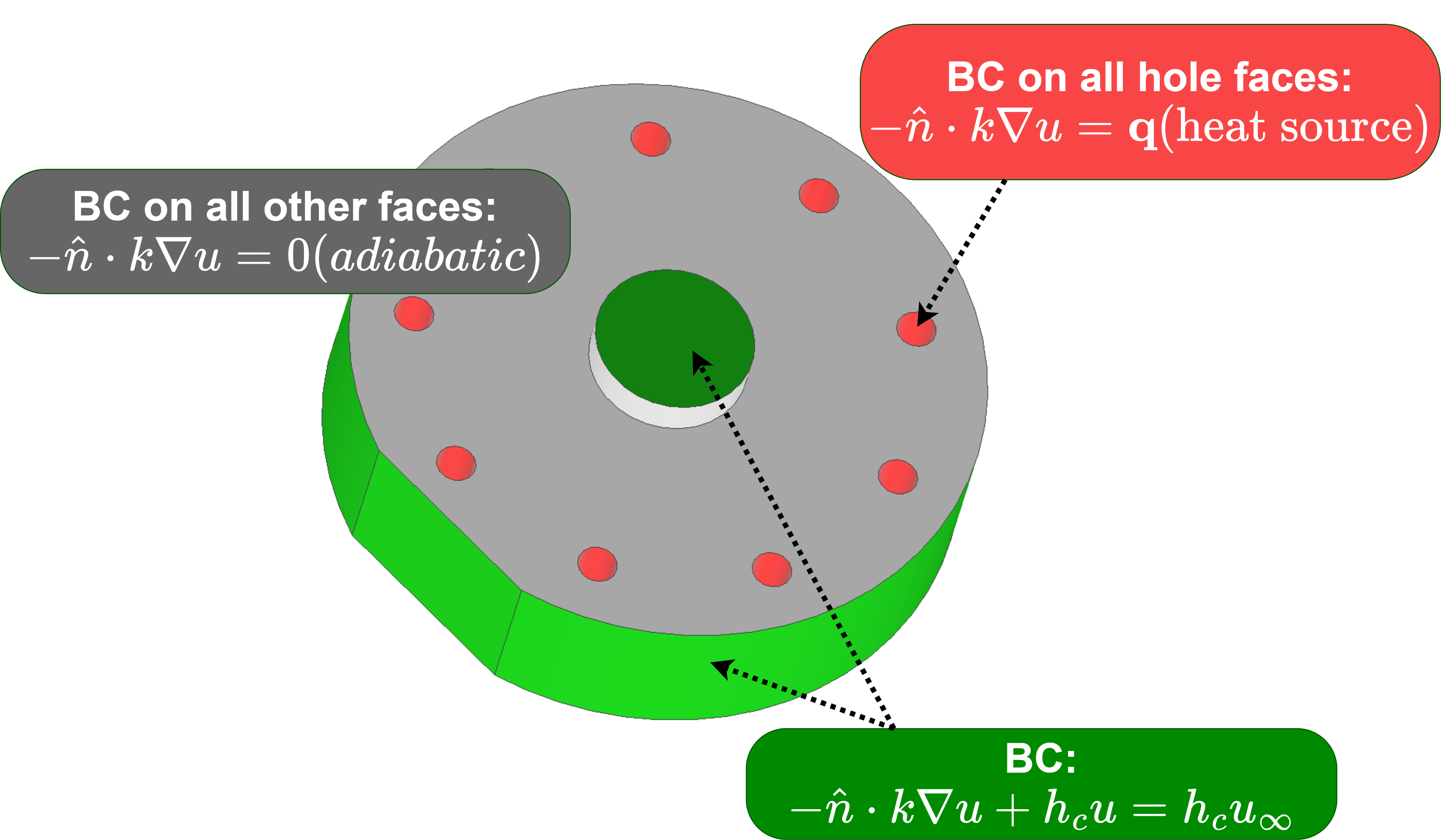
where is the thermal conductivity, is the internal heat source, and is the spatially varying temperature field. For multi-task operator learning, we solve this equation on a parametric D circular plate as outlined in [43]. The plate has an outer diameter of inches, a central protrusion of height inch, and an overall thickness of inch. The location and the number of holes are parameterized as follows: the holes are placed at distances inches from the center of the protrusion, with the number of holes varying between and . All holes are equispaced in all the considered geometries, while the location of one hole is fixed in all the geometries in the plate (see Figure 10(a)). The radial location of the holes, is varied in steps of inch. Heat sources are placed in each hole, with a convective heat flux on the protrusion and side face, and adiabatic conditions elsewhere. These natural convective boundary conditions are shown in Figure 10(b). The objective is to learn the temperature distribution across the geometries that result from combinations of and (details of data generation in Section S1.3). Figure 11 presents four representative geometries and the corresponding temperature fields obtained from MATLAB’s PDE Toolbox.
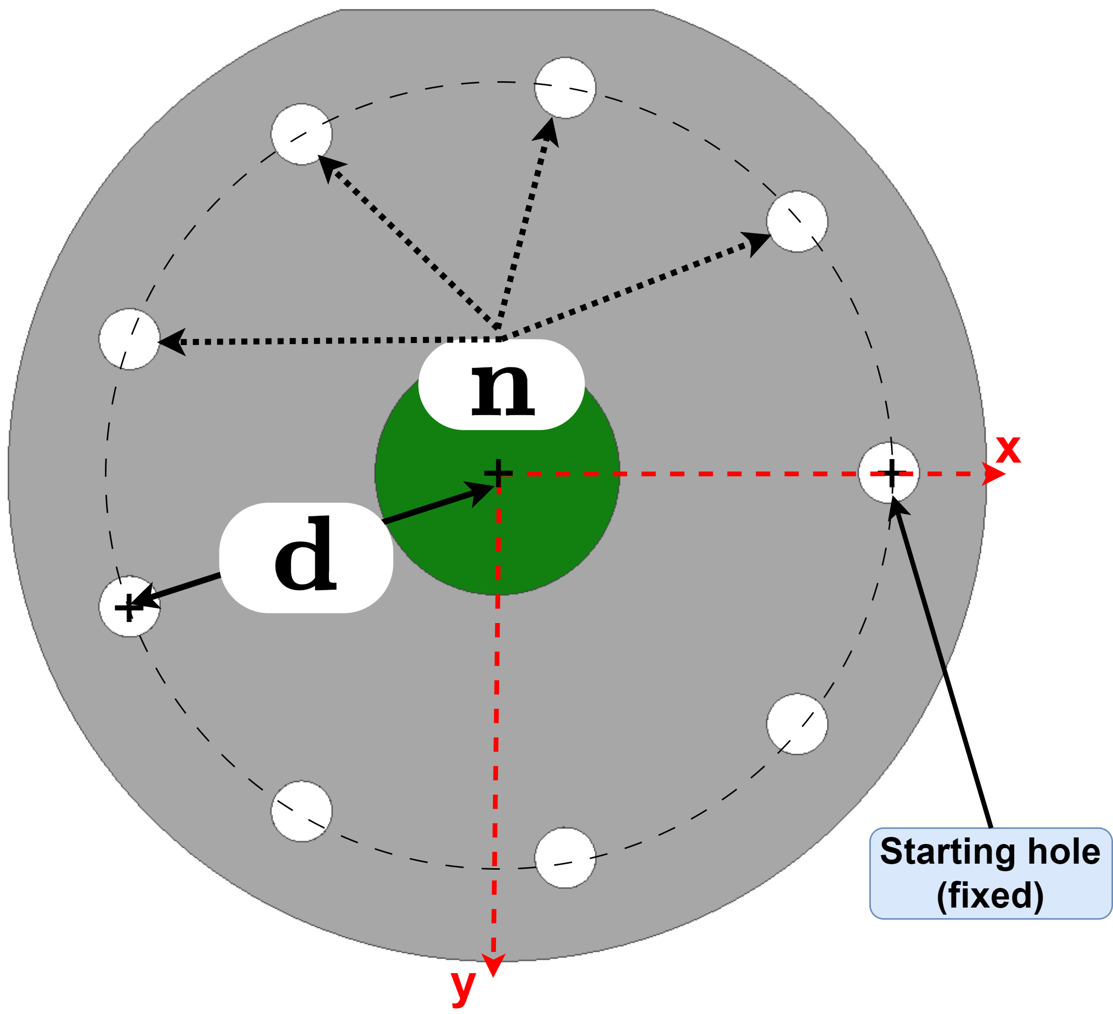


Our objective here is to learn the operator mapping between the geometry parameters defining the different plate configurations and the resulting temperature field due to the heat sources placed inside the holes located in the plate. Since the number and location of the holes change based on the parameters and , the resulting temperature field varies for each plate configuration. For the operator learning purpose, we select a total of training samples that encompass the minimum, maximum, and median values of the parameter for different numbers of holes. For instance, for a plate with , we choose three samples with holes located at , , and as training samples corresponding to . The sample choice ensures that the extreme ends of the design space are well represented in the training dataset while avoiding oversampling. The remaining geometries are used as test cases for network inference. A list of the cases used for training and testing is provided in Table S1.
The parametric representation for the plate ( and ) is used as input to our branch network, while the trunk network receives uniformly sampled points in the domain as input. Unlike the previous example on the 2D Darcy problem where the binary mask was considered as input to the branch network, here only the geometry parametrization values are employed. The binary mask is used as additional information in the loss function. We utilize the same grid points for all plate configurations with the trunk network and later apply a binary mask to constrain the temperature field to be zero outside the geometry, similar to the D Darcy problem. The masking matrix is a D grid with values of (outside) and (inside) the domain boundary. By utilizing this binary mask, we establish the associativity between the grid points and geometry points, enabling the operator network to learn the temperature field across multiple geometries simultaneously. The training step employs an exponentially decaying learning rate, starting at with a decay rate of every iterations.
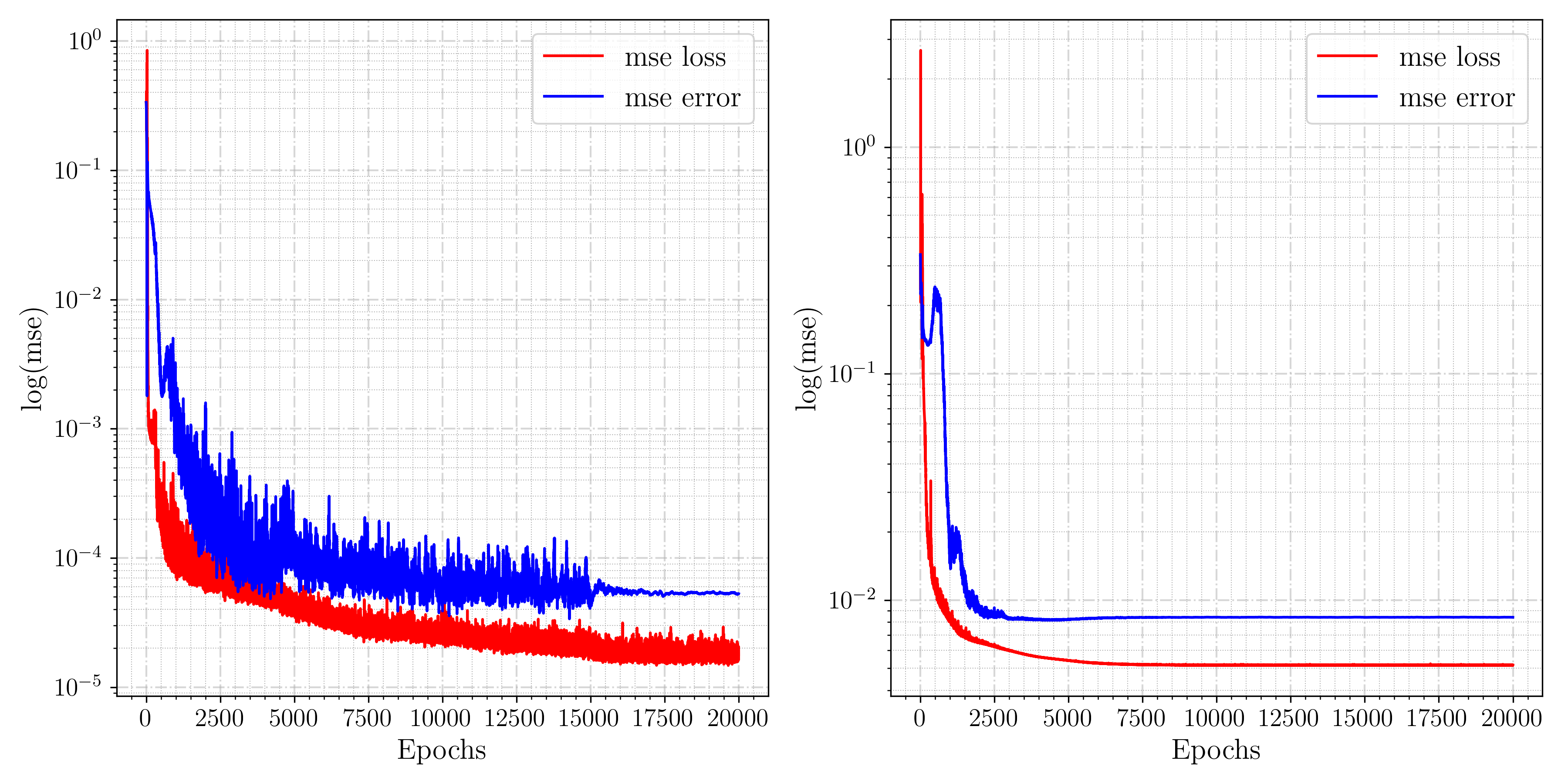
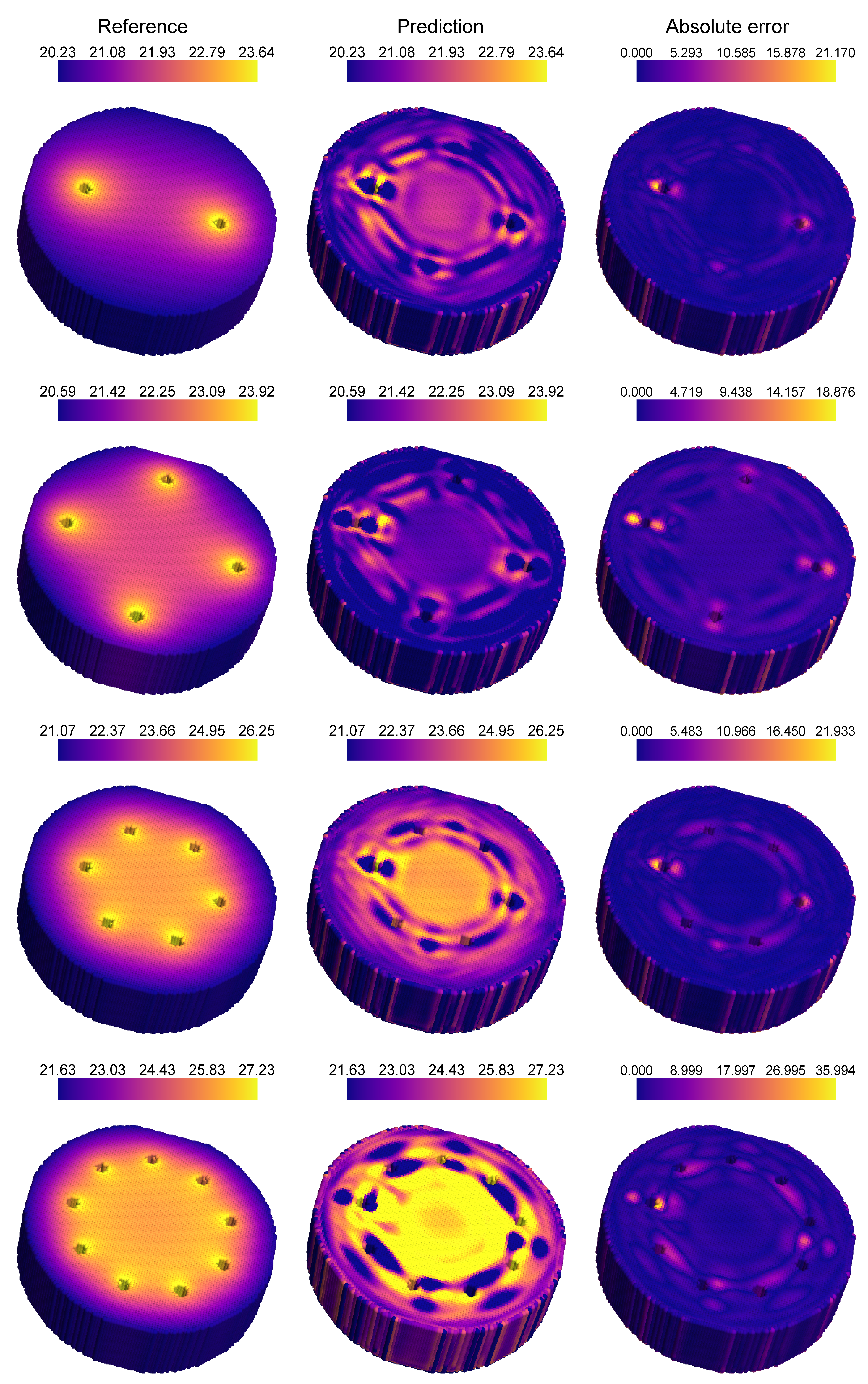
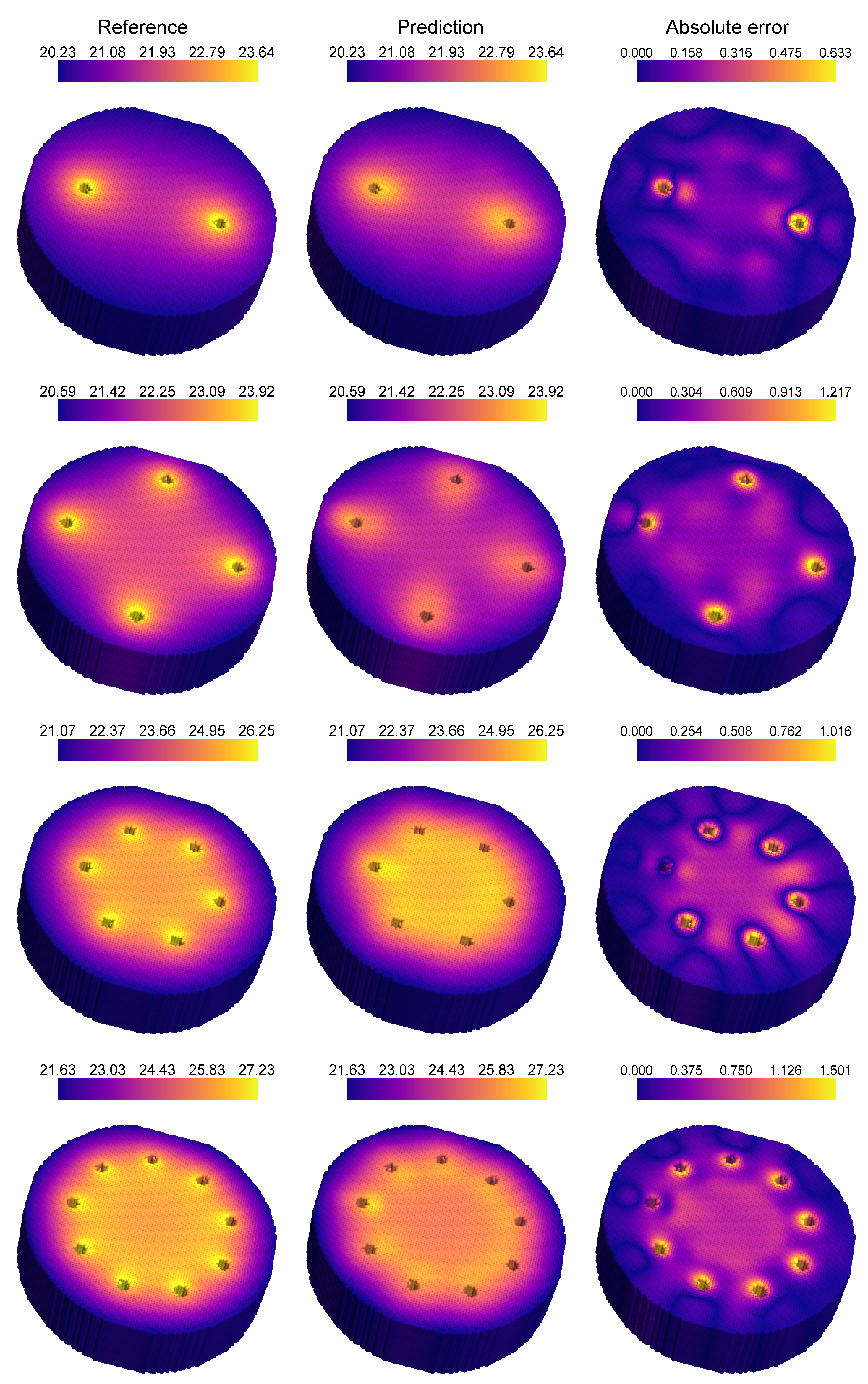
The binary mask, applied to the network output, ensures that the solution at points outside the geometry is zero, thereby improving convergence and accuracy. Figure 12 compares the convergence of the MT-DeepONet with and without the masking function in the loss function. The application of a mask to the solution output demonstrates better error convergence. Figure 13 shows the prediction of MT-DeepONet without the masking operation, where higher inaccuracies are observed across the domain due to insufficient geometry representation in the training dataset. Applying a binary mask imposes an extra constraint that assists the network in learning solutions across different geometries. This masking process supplies essential geometric details and improves the network’s capacity to generalize to new plate configurations (with the same ). Figure 14 presents representative examples of geometries comparing the reference temperature field with the network prediction. These predictions align well with the reference numerical solution. Higher error values are observed near the holes due to their being under-represented in the training data. We observed better results when more geometries are added to the training dataset but this leads to oversampling in the training dataset. The masking framework functions similarly to transfer learning between tasks, albeit without involving network re-training, and is critical for predicting solutions across different geometries in our experiments.
4 Summary
In this work, we introduced the multi-task deep operator network (MT-DeepONet), which learns across multiple scenarios, including different geometries and physical systems, within a single training session. The framework is capable of handling diverse physical processes as demonstrated with the Fisher equation and Darcy flow examples. The MT-DeepONet framework shows a strong ability to map operator solutions across multiple geometries. Thus, the MTL-DeepONet demonstrates significant capabilities in learning and transferring knowledge across varied PDE forms and geometric configurations. While achieving competitive accuracy in predicting solutions, challenges such as managing negative interference between tasks and generalizing to unseen geometries were evident, particularly in the context of learning multiple varied geometries. The binary mask function introduced in the loss term imposes the boundary condition on different geometries as well as improves convergence and generalization. Future research directions should include optimizing network architectures to enhance transfer learning efficacy, developing robust methods for encoding complex D geometries, and exploring advanced techniques to mitigate negative inference in MT-DeepONet.
Acknowledgements
The authors would like to acknowledge computing support provided by the Advanced Research Computing at Hopkins (ARCH) core facility at Johns Hopkins University and the Rockfish cluster and the computational resources and services at the Center for Computation and Visualization (CCV), Brown University where all experiments were carried out.
Funding
VK & GEK: U.S. Department of Energy project Sea-CROGS (DE-SC0023191) and the OSD/AFOSR Multidisciplinary Research Program of the University Research Initiative (MURI) grant FA9550-20-1-0358.
KK: U.S. Department of Energy, Office of Science, Office of Advanced Scientific Computing Research grant under Award Number DE-SC0020428.
SG & MDS: U.S. Department of Energy, Office of Science, Office of Advanced Scientific Computing Research grant under Award Number DE-SC0024162.
Author contributions
Conceptualization: SG, KK, GEK, MDS
Investigation: SG, VK, KK
Visualization: VK, SG
Supervision: GEK, MDS
Writing—original draft: VK, SG
Writing—review & editing: VK, SG, KK, GEK, MDS
Data and code availability
All codes and datasets will be made publicly available at https://github.com/varunsingh88/MTL_DeepONet.git upon publication.
Competing interests
Karniadakis has financial interests with the company PredictiveIQ. The rest of the authors declare no competing interests.
References
- [1] L. Lu, X. Meng, S. Cai, Z. Mao, S. Goswami, Z. Zhang, G. E. Karniadakis, A comprehensive and fair comparison of two neural operators (with practical extensions) based on FAIR data, Computer Methods in Applied Mechanics and Engineering 393 (2022) 114778.
- [2] S. Goswami, A. Bora, Y. Yu, G. E. Karniadakis, Physics-Informed Deep Neural Operator Networks, in: Machine Learning in Modeling and Simulation: Methods and Applications, Springer, 2023, pp. 219–254.
- [3] L. Lu, P. Jin, G. Pang, Z. Zhang, G. E. Karniadakis, Learning nonlinear operators via DeepONet based on the universal approximation theorem of operators, Nature machine intelligence 3 (3) (2021) 218–229.
- [4] Z. Li, N. Kovachki, K. Azizzadenesheli, B. Liu, K. Bhattacharya, A. Stuart, A. Anandkumar, Fourier Neural Operator for Parametric Partial Differential Equations, arXiv preprint arXiv:2010.08895 (2020).
- [5] T. Tripura, S. Chakraborty, Wavelet neural operator for solving parametric partial differential equations in computational mechanics problems, Computer Methods in Applied Mechanics and Engineering 404 (2023) 115783.
- [6] Q. Cao, S. Goswami, G. E. Karniadakis, Laplace neural operator for solving differential equations, Nature Machine Intelligence (2024) 1–10.
- [7] B. Raonic, R. Molinaro, T. Rohner, S. Mishra, E. de Bezenac, Convolutional Neural Operators, in: ICLR 2023 Workshop on Physics for Machine Learning, 2023.
- [8] R. Caruana, Multitask Learning, Machine learning 28 (1997) 41–75.
- [9] P. Liu, X. Qiu, X. Huang, Deep multi-task learning with shared memory, arXiv preprint arXiv:1609.07222 (2016).
- [10] M. Long, H. Zhu, J. Wang, M. I. Jordan, Deep transfer learning with joint adaptation networks, in: International conference on machine learning, PMLR, 2017, pp. 2208–2217.
- [11] D. Xu, W. Ouyang, X. Wang, N. Sebe, Pad-net: Multi-tasks guided prediction-and-distillation network for simultaneous depth estimation and scene parsing, in: Proceedings of the IEEE conference on computer vision and pattern recognition, 2018, pp. 675–684.
- [12] S. Liu, E. Johns, A. J. Davison, End-to-end multi-task learning with attention, in: Proceedings of the IEEE/CVF conference on computer vision and pattern recognition, 2019, pp. 1871–1880.
- [13] I. Misra, A. Shrivastava, A. Gupta, M. Hebert, Cross-stitch networks for multi-task learning, in: Proceedings of the IEEE conference on computer vision and pattern recognition, 2016, pp. 3994–4003.
- [14] S. Reed, K. Zolna, E. Parisotto, S. G. Colmenarejo, A. Novikov, G. Barth-Maron, M. Gimenez, Y. Sulsky, J. Kay, J. T. Springenberg, et al., A generalist agent, arXiv preprint arXiv:2205.06175 (2022).
- [15] L. Yang, S. Liu, T. Meng, S. J. Osher, In-context operator learning with data prompts for differential equation problems, Proceedings of the National Academy of Sciences 120 (39) (2023) e2310142120.
- [16] S. Goswami, K. Kontolati, M. D. Shields, G. E. Karniadakis, Deep transfer operator learning for partial differential equations under conditional shift, Nature Machine Intelligence 4 (12) (2022) 1155–1164.
- [17] T. Chen, H. Chen, Universal approximation to nonlinear operators by neural networks with arbitrary activation functions and its application to dynamical systems, IEEE Transactions on Neural Networks 6 (4) (1995) 911–917.
- [18] P. C. Di Leoni, L. Lu, C. Meneveau, G. Karniadakis, T. A. Zaki, DeepONet prediction of linear instability waves in high-speed boundary layers, arXiv preprint arXiv:2105.08697 (2021).
- [19] K. Kontolati, S. Goswami, M. D. Shields, G. E. Karniadakis, On the influence of over-parameterization in manifold based surrogates and deep neural operators, Journal of Computational Physics (2023) 112008.
- [20] S. Goswami, M. Yin, Y. Yu, G. E. Karniadakis, A physics-informed variational DeepONet for predicting crack path in quasi-brittle materials, Computer Methods in Applied Mechanics and Engineering 391 (2022) 114587.
- [21] V. Oommen, K. Shukla, S. Goswami, R. Dingreville, G. E. Karniadakis, Learning two-phase microstructure evolution using neural operators and autoencoder architectures, npj Computational Materials 8 (1) (2022) 190.
- [22] Q. Cao, S. Goswami, T. Tripura, S. Chakraborty, G. E. Karniadakis, Deep neural operators can predict the real-time response of floating offshore structures under irregular waves, Computers & Structures 291 (2024) 107228.
- [23] M. L. Taccari, H. Wang, S. Goswami, M. De Florio, J. Nuttall, X. Chen, P. K. Jimack, Developing a cost-effective emulator for groundwater flow modeling using deep neural operators, Journal of Hydrology 630 (2024) 130551.
- [24] N. Borrel-Jensen, S. Goswami, A. P. Engsig-Karup, G. E. Karniadakis, C.-H. Jeong, Sound propagation in realistic interactive 3d scenes with parameterized sources using deep neural operators, Proceedings of the National Academy of Sciences 121 (2) (2024) e2312159120.
- [25] S. De, M. Hassanaly, M. Reynolds, R. N. King, A. Doostan, Bi-fidelity Modeling of Uncertain and Partially Unknown Systems using DeepONets, arXiv preprint arXiv:2204.00997 (2022).
- [26] L. Lu, R. Pestourie, S. G. Johnson, G. Romano, Multifidelity deep neural operators for efficient learning of partial differential equations with application to fast inverse design of nanoscale heat transport, arXiv preprint arXiv:2204.06684 (2022).
- [27] A. A. Howard, M. Perego, G. E. Karniadakis, P. Stinis, Multifidelity Deep Operator Networks, arXiv preprint arXiv:2204.09157 (2022).
- [28] P. Jin, S. Meng, L. Lu, MIONet: Learning multiple-input operators via tensor product, SIAM Journal on Scientific Computing 44 (6) (2022) A3490–A3514.
- [29] S. Goswami, D. S. Li, B. V. Rego, M. Latorre, J. D. Humphrey, G. E. Karniadakis, Neural operator learning of heterogeneous mechanobiological insults contributing to aortic aneurysms, Journal of the Royal Society Interface 19 (193) (2022) 20220410.
- [30] E. Zhang, A. Kahana, E. Turkel, R. Ranade, J. Pathak, G. E. Karniadakis, A Hybrid Iterative Numerical Transferable Solver (HINTS) for PDEs Based on Deep Operator Network and Relaxation Methods, arXiv preprint arXiv:2208.13273 (2022).
- [31] A. Kahana, E. Zhang, S. Goswami, G. Karniadakis, R. Ranade, J. Pathak, On the geometry transferability of the hybrid iterative numerical solver for differential equations, Computational Mechanics 72 (3) (2023) 471–484.
- [32] B. Bahmani, S. Goswami, I. G. Kevrekidis, M. D. Shields, A Resolution Independent Neural Operator, arXiv preprint arXiv:2407.13010 (2024).
- [33] S. Goswami, K. Kontolati, M. D. Shields, G. E. Karniadakis, Deep transfer operator learning for partial differential equations under conditional shift, Nature Machine Intelligence (2022) 1–10.
- [34] S. Wang, H. Wang, P. Perdikaris, Learning the solution operator of parametric partial differential equations with physics-informed DeepONets, Science advances 7 (40) (2021) eabi8605.
- [35] L. Mandl, S. Goswami, L. Lambers, T. Ricken, Separable DeepONet: Breaking the Curse of Dimensionality in Physics-Informed Machine Learning, arXiv preprint arXiv:2407.15887 (2024).
- [36] K. Kontolati, S. Goswami, G. Em Karniadakis, M. D. Shields, Learning nonlinear operators in latent spaces for real-time predictions of complex dynamics in physical systems, Nature Communications 15 (1) (2024) 5101.
- [37] R. A. Fisher, The wave of advance of advantageous genes, Annals of eugenics 7 (4) (1937) 355–369.
- [38] V. M. Tikhomirov, Selected Works of AN Kolmogorov: Volume I: Mathematics and Mechanics, Vol. 25, Springer Science & Business Media, 1991.
- [39] Z. Zhang, Z. Zou, E. Kuhl, G. E. Karniadakis, Discovering a reaction–diffusion model for Alzheimer’s disease by combining PINNs with symbolic regression, Computer Methods in Applied Mechanics and Engineering 419 (2024) 116647.
- [40] J. Patade, S. Bhalekar, Approximate analytical solutions of newell-whitehead-segel equation using a new iterative method, World Journal of Modelling and Simulation 11 (2) (2015) 94–103.
- [41] Y. Zeldovich, Flame propagation in a substance reacting at initial temperature, Combustion and Flame 39 (3) (1980) 219–224.
- [42] J. He, S. Koric, D. Abueidda, A. Najafi, I. Jasiuk, Geom-DeepONet: A point-cloud-based deep operator network for field predictions on 3D parameterized geometries, Computer Methods in Applied Mechanics and Engineering 429 (2024) 117130.
- [43] Paul, 3D Finite Element Analysis with MATLAB, https://www.mathworks.com/matlabcentral/fileexchange/50482-3d-finite-element-analysis-with-matlab, online; accessed 3 July 2024 (2024).
Supplementary information
S1 Data Generation
In this section, we present relevant details related to the data generation process for the three problems investigated in this study.
S1.1 Fisher equations
For this problem, the goal is to learn the operator mapping from the random initial density condition across a parameter range and , as defined in Table 1, for its entire time evolution. This mapping is expressed as , where and . The initial density is modeled as a Gaussian random field (GRF), defined by:
| (15) |
where and are the mean and covariance functions, respectively. We set , while the covariance matrix is defined by the squared exponential kernel:
| (16) |
where is the correlation length, and is the variance. We utilize Karhunen-Loéve expansion (KLE) to generate random initial conditions. The temporal points and spatial points are discretized into a grid, resulting in a total of 1,280 collocation points. Parameters and are discretized in steps of and , respectively, within the defined parameter space. Combining different parameter values for and with the random initial conditions, we generate a total of training samples. This dataset is split into training and testing sets using an split, with and . For preparing data for the multi-task operator network, we concatenate the initial condition data at domain points with the parameter values for the three Fisher equations defined in Table 1, resulting in a dimensional input vector ( initial condition points + equation parameters).
S1.2 Darcy equation with transfer learning across multiple geometries
The multi-task objective in this problem is to learn the operator for the Darcy flow equation described in Equation 12 over different D spatial domains under randomly generated initial states for conductivity field . The hydraulic conductivity field is modeled as a stochastic process, using truncated Karhunen-Loéve expansion. The conductivity field is generated in a reference square domain with grid points using a Gaussian random field with length scale, . A total of solution fields are generated using the multiple initial values of conductivity fields for each geometry. A Dirichlet boundary condition of is applied on all the edges of each geometry, shown in Figure 5. The solution to Darcy’s equation for all samples is generated using MATLAB’s PDE Toolbox solver. The domain mesh is generated using the MATLAB PDE Toolbox mesh generation algorithm with a maximum mesh size of inches for all geometries. We use unstructured triangular elements for the mesh. The hydraulic pressure head solution obtained is linearly interpolated on a regular grid in to utilize a common trunk network input. Points in the square grid that lie outside the triangular geometry are extracted and the solution field at such points is manually set to throughout the dataset. We sub-divide the samples into and for each source model. For training the MT-DeepONet with multiple geometries, we use an equal number of samples from each geometry to obtain a combined total of , thus ensuring equal representation.
S1.3 Heat transfer equation with multiple D geometry
To generate data for the steady-state heat transfer problem with multiple plate geometries, we create a parametric CAD model of the plate where the parameters and determine the number of holes and their location relative to the central axis of the plate protrusion (see Figure 10), respectively. To generate unique geometries with a combination of and , we fix the location of one hole across all the geometries (see Figure 10(a)). We solve the steady-state heat transfer Equation 14 using MATLAB’s PDE Toolbox for various design configurations that result from varying the design parameters and in the plate geometry, where and . We increment in steps of 0.1 resulting in a total of distinct design configurations. As discussed earlier, we separate the training and test cases based on the hole location, as shown in Table S1. For each design, we use PDEToolbox for mesh generation with a maximum element size of inch and tetrahedral elements. A heat source is placed inside each hole, simulating a cartridge heater to heat the plate. Convective boundary conditions are applied on the protruding face and side walls with an ambient temperature and a convective heat transfer coefficient . The output solution, which is the temperature field , is evaluated at all node points of the mesh. Figure 11 shows representative examples of the different geometries and their corresponding temperature fields obtained by solving Equation 14. The temperature solutions are initially obtained on unstructured grid points. For simplifying the inputs for the trunk network, we interpolate these solutions over a regular D grid () around the plate. Points in the regular grid that fall outside the domain of the plate are set to before training the network.
| n | d (training samples) | d (testing samples) |
|---|---|---|
| 2 | {0.9, 1.2, 1.6} | {1.0, 1.1, 1.3, 1.4, 1.5} |
| 3 | {0.9, 1.2, 1.6} | {1.0, 1.1, 1.3, 1.4, 1.5} |
| 4 | {0.9, 1.2, 1.6} | {1.0, 1.1, 1.3, 1.4, 1.5} |
| 5 | {0.9, 1.2, 1.6} | {1.0, 1.1, 1.3, 1.4, 1.5} |
| 6 | {0.9, 1.2, 1.6} | {1.0, 1.1, 1.3, 1.4, 1.5} |
| 7 | {0.9, 1.2, 1.6} | {1.0, 1.1, 1.3, 1.4, 1.5} |
| 8 | {0.9, 1.2, 1.6} | {1.0, 1.1, 1.3, 1.4, 1.5} |
| 9 | {0.9, 1.2, 1.6} | {1.0, 1.1, 1.3, 1.4, 1.5} |
S2 Data pre-processing
The multi-task operator network design for all the four problems discussed earlier consists of a branch and trunk network, where the branch creates a map between the varying input functions (equation representations, geometry, initial conditions) and the output function. The inputs to the branch network are formed by combining the feature representations of the input functions. The input to the trunk network for the Fisher problem consists of spatio-temporal locations , where . For the Darcy and D heat transfer problem, the trunk input consists only of spatial points where . To improve network training, the available data is scaled to reduce to the same order. In particular, the input initial condition and outputs for Darcy, and Fisher problems are scaled using the mean and standard deviation of the training dataset using the operation:
| (17) |
For the D heat transfer problem, we normalize the inputs and outputs using min-max scaling given by:
| (18) |
where and represent the minimum and maximum values across the sample set.
S3 Network Architecture
Our network design and hyper-parameter selection are determined by the problem under investigation. In Table S3, we provide a summary of the network architecture and hyper-parameters used for different problems in this study.
| Problem | Branch network | Trunk network | |||||
|---|---|---|---|---|---|---|---|
| (neurons per layer) | Activation | Regularizer | Dropout | ||||
| (branch) | Masking | ||||||
| Type | Neurons per layer | ||||||
| Fisher | MLP | [68, 128, 128, 300] | [2, 128, 128, 128, 300] | Leaky_ReLU | None | None | |
| Darcy | 2D CNN | ||||||
| MLP | CNN filters: [16, 32, 64, 64] | ||||||
| MLP: [128, 128, 150] | [2, 128, 128, 150] | Conv: Tanh, ReLU | |||||
| MLP: Leaky_ReLU | None | 0.1 | Yes | ||||
| 3D heat transfer | MLP | [2, 32, 64, 128, 128, 200] | [3, 32, 64 3, 128 5, 200] | swish | None | 0.1 | Yes |