Systematic analysis of strange single heavy baryons and
Abstract
Motivated by the experimental progress in the study of heavy baryons, we investigate the mass spectra of strange single heavy baryons in the -mode, where the relativistic quark model and the infinitesimally shifted Gaussian basis function method are employed. It is shown that the experimental data can be well reproduced by the predicted masses. The root mean square radii and radial probability density distributions of the wave functions are analyzed in detail. Meanwhile, the mass spectra allow us to successfully construct the Regge trajectories in the plane. We also preliminarily assign quantum numbers to the recently observed baryons, including , , , , , , , , , , and . At last, the spectral structure of the strange single heavy baryons is shown. Accordingly, we predict several new baryons that might be observed in forthcoming experiments.
Key words: Single heavy baryons, Mass spectra, Relativistic quark model.
pacs:
13.25.Ft; 14.40.LbI. Introduction
In recent years, many single heavy baryons have been observed in experiments, and the mass spectra of single heavy baryon families have become more and more abundant art77 ; art210 ; art81 ; art24 ; art25 ; art30 ; art83 ; art201 ; art202 ; art84 ; art85 ; art31 ; art29 ; art88 ; art601 ; art87 ; art203 ; art204 ; art89 ; art78 ; art79 ; art130 ; art15 ; art18 ; art120 ; art16 ; art125 ; art2 ; art90 ; art213 ; art126 . Such a wealth of experimental data gives theorists an opportunity to test the validity of current theoretical frameworks. Additionally, this is also a good time to carry out a systematic and precise calculation with some theoretical methods, so as to promote the consistency between the experiments and theories.
The strange single heavy baryon families including () art81 ; art210 ; art30 ; art25 ; art31 ; art29 ; art83 ; art84 ; art85 ; art88 ; art89 ; art87 ; art120 ; art125 ; art213 and () art77 ; art201 ; art202 ; art203 ; art204 ; art78 ; art79 ; art15 ; art130 ; art90 ; art126 , are being established step by step with the cooperative efforts of experimentalists and theorists. So far, more than a dozen baryons have been recorded in the latest particle data group (PDG) art2 , even though the values of some baryons are still undetermined, such as , and . Recently, some other baryons have been observed in experiment, including art31 , art120 , , , art125 , and art126 . Accordingly, there have been a lot of theoretical studies on these baryons, such as art309 ; art44 ; art322 ; art23 ; art128 , art23 ; art45 ; art70 ; art311 , (including and ) art321 , art32 , art27 ; art46 ; art305 ; art901 ; art902 ; art903 , (3123) art310 , art319 ; art318 ; art313 ; art306 ; art316 , art129 ; art317 and () art320 . In order to identify their quantum numbers and assign them suitable positions in the mass spectra, it is necessary to systematically investigate their spectroscopies.
In recent decades, the heavy baryons have been studied by many theoretical methods, including the quark potential model in the heavy quark-light diquark picture art5 ; art1 ; art35 ; art36 ; art310 , relativistic quark model art4 , harmonic oscillator quark model art321 , constituent quark model art28 ; art94 ; art95 ; art119 , chiral quark model art32 ; art309 ; art319 ; art320 , chiral perturbation theory art37 ; art38 ; art39 ; art40 ; art41 , relativistic flux tube model art27 , Bethe-Salpeter formalism art42 , effective Lagrangian approach art318 , decay model art33 ; art34 ; art43 ; art47 ; art48 ; art49 ; art50 ; art76 , lattice QCD art51 ; art52 ; art53 ; art54 , bound state picture art55 , light cone QCD sum rules art56 ; art57 ; art58 ; art59 ; art60 ; art61 ; art62 ; art63 ; art64 ; art65 , and QCD sum rules method art66 ; art67 ; art68 ; art69 ; art71 ; art72 ; art73 ; art74 ; art75 ; art308 .
In particular, it is worth mentioning that Ebert art5 ; art1 put forward a heavy quark-light diquark picture in the framework of a QCD-motivated relativistic quark model, in which an initial three-body problem is reduced to a two-step two-body problem. They systematically studied the spectroscopy and Regge trajectories of heavy baryons, and have achieved a great success in predicting new singly heavy baryons. Because the excited states in the heavy quark-light diquark picture are very similar to those of the -mode in a three-quark system art28 , it would be interesting to investigate the -mode in a three-quark system systematically and study the difference in mass spectra between this mode and the heavy quark-light diquark picture.
In the 1980s, Godfrey and Isgur developed a relativistic quark model by which they studied mass spectra of mesons art91 . Then, Capstick and Isgur extended it to the study of baryons art4 . In the relativistic quark model, the Hamiltonian contains almost all of the interactions between two quarks, which is expected to give accurate calculations for heavy baryon spectra.
The Gaussian expansion method (GEM) and the infinitesimally-shifted Gaussian (ISG) basis functions art92 have been successfully applied to few-body systems in nuclear physics. ISG method has great advantages to improve the computational accuracy and efficiency in the calculation of few-body systems. In recent years, they were introduced in the study of heavy baryons art28 ; art94 ; art95 , tetraquarks art93 ; art96 ; art97 and pentaquarks art115 .
Inspired by the above discussion, we try to combine the relativistic quark model with the ISG method, so as to investigate the strange single heavy baryon spectra in a three-quark system. For the excited states, we would only focus on the -mode and compare the results with those of the heavy quark-light diquark picture and the relevant experimental data as well. The present work is a preliminary attempt to systematically investigate strange single heavy baryon spectra and this method is promising to be used in the study of other multi-quark systems, including the exotic ones art801 ; art802 ; art803 ; art804 ; art805 .
This paper is organized as follows. In Sect.II, we briefly describe the methods used in the theoretical calculations, mainly including the relativistic quark model and the GEM(ISG) method. In Sect.III, we present the root mean square radii and the mass spectra of the baryons, analyze the radial probability distributions, and construct the Regge trajectories. On these bases, we perform a detailed analysis of the baryons that have been of interest recently. At last, the mass spectral structures are displayed. And Sect.IV is reserved for our conclusions.
II. Phenomenological methods adopted in this work
2.1 Relativistic quark model and Jacobi coordinates
The relativistic quark model is based on the hypothesis that baryons may be approximately described in terms of center-of-mass (CM) frame valence-quark configurations, the dynamics of which are governed by a Hamiltonian with a one-gluon exchange dominant component at short distances and with a confinement implemented by a flavor-independent Lorentz-scalar interaction art4 . For a three-quark system the Hamiltonian reads,
| (1) |
| (2) |
| (3) |
where , and are the confinement, spin-orbit and hyperfine interactions, respectively. The confinement item includes one-gluon exchange potentials and the linear confined potentials. Due to the relativistic effect, the interactions should be modified with CM momentum-dependent factors. It is worth noting that the forms of the interactions in this paper have been rearranged for ease of use art116 ; art93 . The interactions are decomposed as follows:
| (4) | |||
| (5) | |||
| (6) |
with
| (7) | |||
| (8) | |||
| (9) | |||
| (10) |
The modified terms in Eqs. (4), (7), (8), (9) and (10) read,
| (11) | |||
| (12) | |||
| (13) | |||
| (14) | |||
| (15) |
where is the relativistic kinetic energy, and is the momentum magnitude of either of the quarks in the CM frame of the quark subsystem art93 .
and are obtained by the smearing transformations of the one-gluon exchange potential and linear confinement potential , respectively,
| (16) |
| (17) |
with
| (18) | |||
| (19) |
Here and are constants. stands for the inner product of the color matrices of quarks and . F includes 8 components (the so-called Gell-mann matrices), which can be written as
| (20) |
with . All of the parameters in these formulas are taken from reference art4 , except that and are revised to be 0.14 GeV2 and -0.198 GeV, respectively.
To represent the internal motion of quarks in a few-body system, one commonly introduces the Jacobi coordinates. As shown in Fig.1, there are totally three channels of Jacobi coordinates for the three-body system. The corresponding Jacobi coordinates are defined as
| (21) | |||
| (22) |
where , , = 1, 2, 3(or replace their positions in turn). and denote the position vector and the mass of the th quark, respectively.
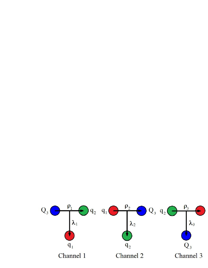
We perform the calculations based on the channel 3. In this case, the 3rd quark is just the heavy quark, which is consistent with the heavy quark limit art118 ; art117 . What is more, (denoted in short as ) is clearly defined as the orbital angular momentum between the light quarks, and (denoted in short as ) represents the one between the heavy quark and the light-quark pair.
2.2 The heavy quark limit and wave function
In the heavy quark limit, the heavy quark within the heavy baryon system is decoupled from the two light quarks. With the requirement of the flavor SU(3) subgroups for the light quarks, the baryons belong to either a sextet of flavor symmetric states , or an antitriplet of the flavor antisymmetric states . The flavor wave functions of strange single heavy baryons are written as,
| (23) |
Here denotes up or down quark, and is charm or bottom quark. is strange quark. For a quantum state with specified angular momenta in this work, the spatial wave function is combined with the spin function as follow.
| (24) |
with , , , . , , , , , and are the quantum numbers which characterize a given quantum state in theory. This scheme (- coupling) is also commonly used to analyze the strong decay of heavy baryons art48 .
2.3 GEM and ISG
In calculations, the spatial wave function in formula (24) should be expanded in a set of basis functions. Naturally, one of the candidates is the simple harmonic oscillator(SHO) basis for its good orthogonality. However, the completeness of the SHO is not rigorous in calculations because a truncated set has to be used art91 ; art4 . Compared to the SHO basis functions, the advantage of the Gaussian basis functions is that they can form an approximately complete set in a finite coordinate space.
Following formula (24), the spatial wave function is expanded in terms of a set of Gaussian basis functions,
| (25) |
where the Gaussian basis function is commonly written in position space as
| (26) |
or in momentum space as
| (27) |
with
| (28) |
, , and are the Gaussian size parameters in the geometric progression for numerical calculations, and the final results are stable and independent of these parameters within an approximately complete set in a sufficiently large space.
The Gaussian basis functions are non-orthogonal, which leads to a generalized matrix eigenvalue problem,
| (29) |
with
| (30) | |||
where , and . and denote the Hamiltonian and the eigenvalue, respectively.
In the calculation of Hamiltonian matrix elements of three-body systems, particularly when complicated interactions are employed, integrations over all of the radial and angular coordinates become laborious even with the Gaussian basis functions. This process can be simplified by introducing the ISG basis functions art92 .
III. Numerical results and discussions
3.1 Numerical stabilities and the -mode
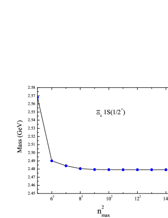
To obtain stable numerical solutions, the Gaussian size parameters set should be optimized. For the Gaussian functions which are a set of non-orthogonal bases in a finite coordinate space, the number of the bases should be in a reasonable range. As shown in Fig.2, the numerical stability is achieved when the dimension parameter falls in the range of , with GeV-1 and GeV-1. is finally adopted in this work, with which both the computation efficiency and accuracy are actually satisfied.
is commonly used to describe a baryon state. If angular momentum , there exist several states under the condition . They may be divided into the following three modes: (1) The -mode with and ; (2) The -mode with and ; (3) The - mixing mode with and .
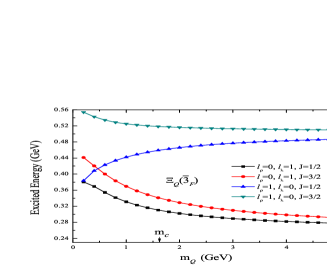
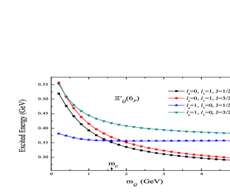
As an example, the excitation energies of the states of as functions of are investigated, where the dependence of excitation energies on of the -mode is compared with that of the -mode. As shown in Fig.3, the -mode and the -mode are clearly separated when increases from 1.0 GeV to 5.0 GeV. In the case of , we come to the same conclusion when GeV as shown in Fig.4. Besides of -wave states, the same feature is also shown in higher angular excited states actually. This conclusion has been obtained in reference art28 . Thus, we investigate the mass spectrum in the -mode.
3.2 Mass spectra, root mean square radius and radial probability density distribution
In this subsection, the root mean square radii, radial probability density distributions and the mass spectra of strange single heavy baryons are presented. For convenience, the relevant experimental data are given together. The detailed results are listed in Tables I-VI (see the appendix). There are a total of four families, namely , , and . The mass spectra of excited states with quantum numbers up to and are displayed. There have been a lot of other theoretical works on this subject art23 ; art70 ; art411 ; art12 ; art318 . Among them, Ebert have studied the heavy baryon spectra with a quark potential model in the heavy quark-light diquark picture art1 . As an important reference, their numerical results are also placed in the tables.
Through the analysis of these calculated results, some general features of the mass spectra are summarized as follows: First, is lower than in energy. This feature has been recognized in light baryons where the highly orbitally excited states have an antisymmetric structure which minimizes the energy art122 ; Second, the mass splitting of spin-doublet states becomes smaller with increasing . For example, Table I shows the mass differences of the spin-doublets of -, -, -, and -wave are 30 MeV, 13 MeV, 5 MeV, and 1 MeV, respectively; Thirdly, for the same , the mass splitting hardly changes with the increase of . For example, Tables II and III show the mass differences of doublets with are 10 MeV, 10 MeV and 13 MeV, respectively; The last, the mass difference between the two adjacent radial excited states gradually decreases with increasing , which is clearly different from that given by Ebert .
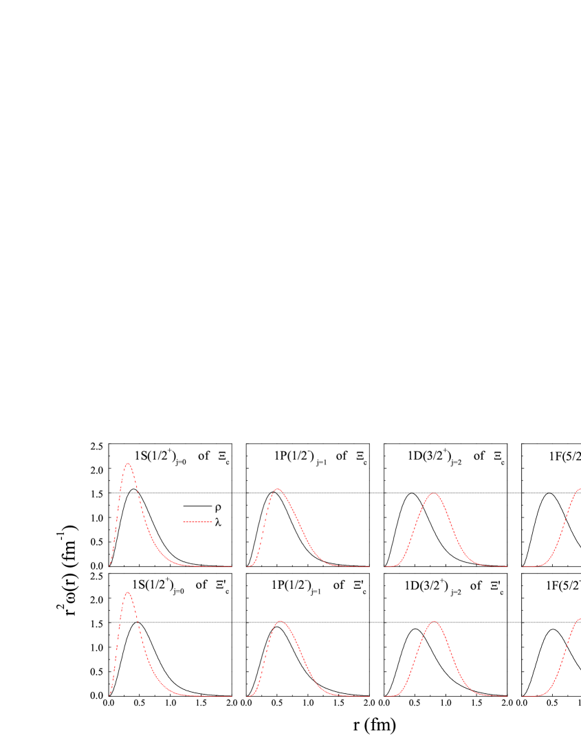
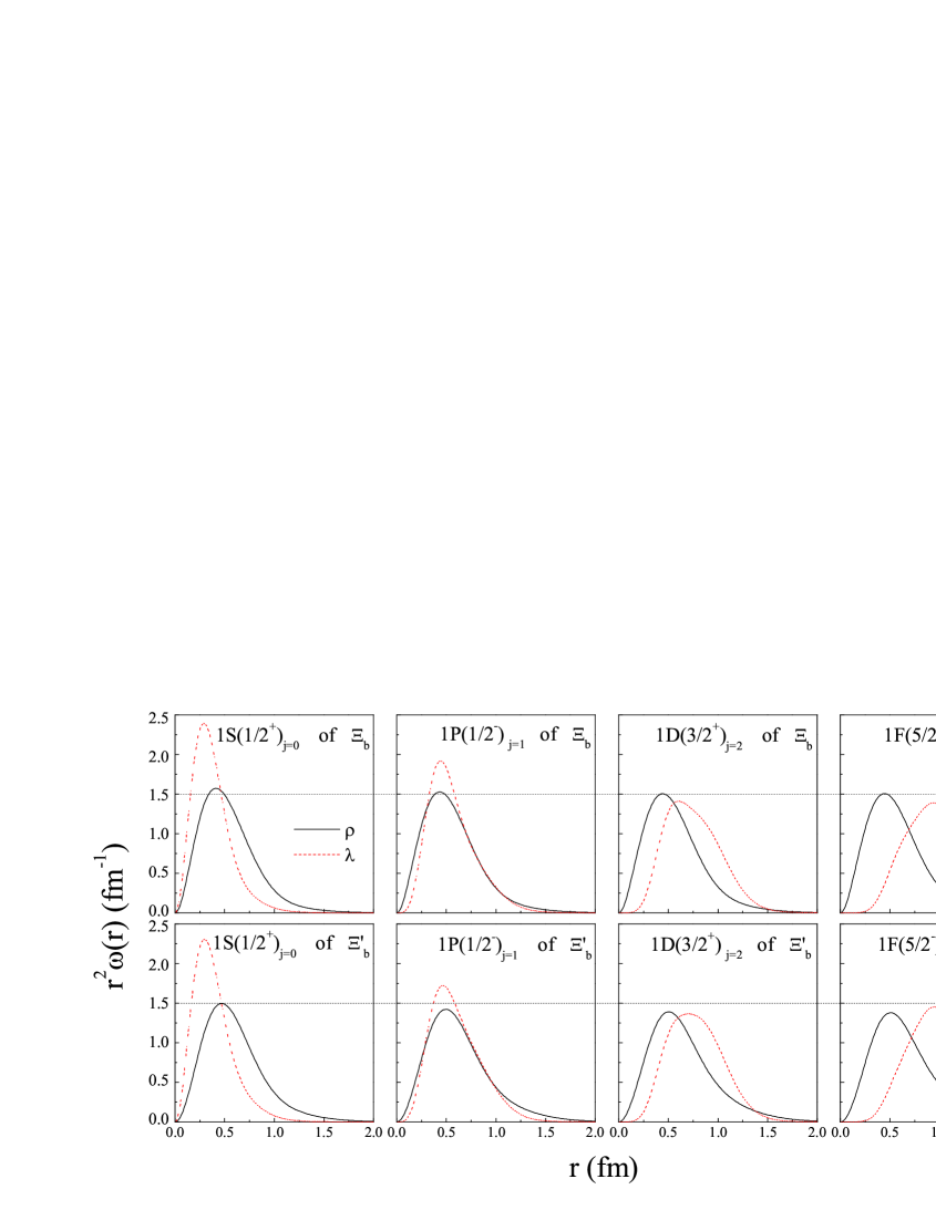
On the other hand, the calculated root mean square radii and radial probability density distributions carry important information. For a three-quark system, the radial probability densities and can be defined as follows,
| (31) |
where and are the solid angles spanned by vectors and , respectively. From Figs.5-7 and tables I-VI, one can find some interesting properties.
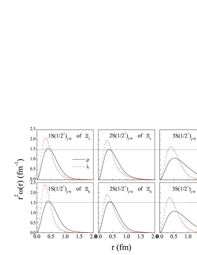
(1) For the same states, when changes from 1 to 4, their values increase small. But their values become larger gradually. The similar phenomenon can be seen in Figs.5 and 6, where the radial probability of changes a little with different values. However, the peak of the significantly shifts outward with increasing .
(2) For the same states, and generally become larger with increasing . And the peaks of their probability densities are generally shifted outward, as shown in Fig.7.
(3) The shapes of the eight black (solid) lines in Fig.5 are almost as same as those in Fig.6. And the values of for the same state are almost the same for () and () families. This reflects the fact that the configurations of the two light quarks in () and () baryons are similar to each other.
(4) As shown in tables I-VI, the root mean square radii of those baryons which have been experimentally well established are generally less than 0.8 fm.
When the root mean square radius becomes larger, the radial probability distribution of the wave function appears more outwardly extended, and the baryons become even looser. Generally speaking, the root mean square radius of a compact baryon might be within a threshold, which is of help to estimate the upper limit of the mass spectrum and constrain the number of members for each heavy baryon family.
3.3 Regge trajectories
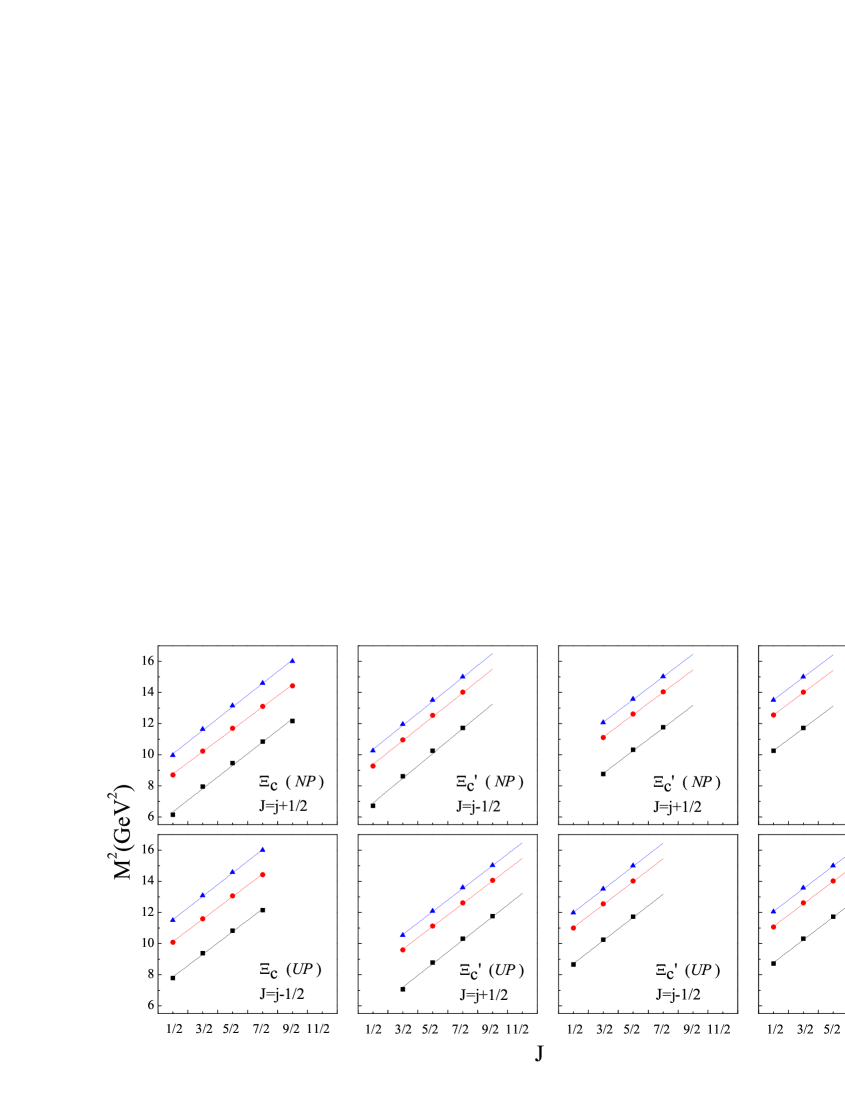
Regge trajectories is an effective method to discribe the hadron mass spectrumart503 ; art504 ; art501 ; art502 ; art505 . In 2011, Ebert constructed the heavy baryon Regge trajectories in both the and the planes art1 .
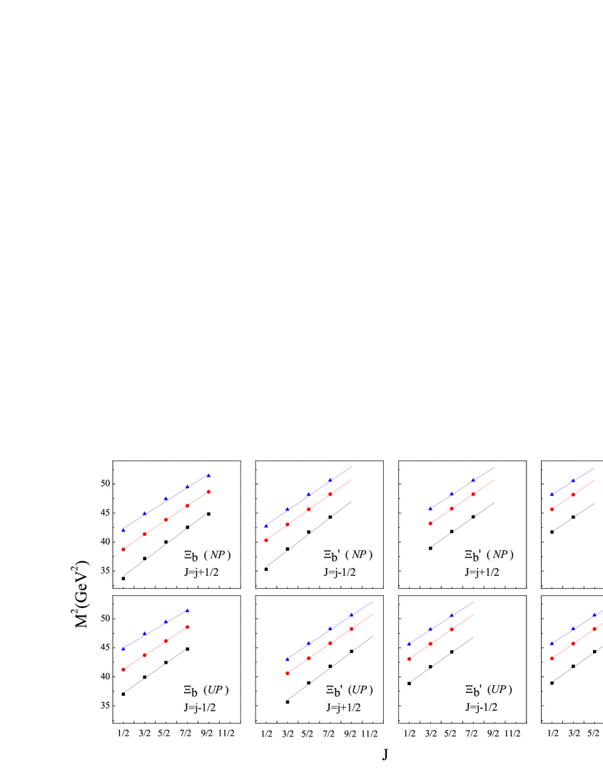
In this subsection, we investigate the Regge trajectories in the plane based on our calculated mass spectra. The states in a baryon family can be classified according to the following parities and angular momenta: (1) Natural and unnatural parities (written in short as and , respectively)art124 ; (2) and (written in short as and ). Thus, the states in the or family are divided into two groups, and the states in the or family are divided into six groups. In this paper, we use the following definition for the Regge trajectories,
| (32) |
where and are the slope and intercept. In Figs. 7 and 8, we plot the Regge trajectories in the plane. The three lines in each figure correspond to the radial quantum number = 1, 2, 3, respectively. The fitted slopes and intercepts of the Regge trajectories are given in Tables VII and VIII.
It is shown that the linear trajectories appear clearly in the plane. All the data points fall on the trajectory lines. This indicates that the Regge trajectory has a strong universality and our theoretical calculations are reliable. These trajectories are almost parallel, but not equidistant, which is an apparent difference between our mass spectra and those in reference art1 .
In this paper, we do not show the Regge trajectories in the plane. In fact, the linear trajectories in the plane can not be constructed from our predicted masses. As will be mentioned in subsection 3.5, if the observation of heavy baryons in forthcoming experiments touched the sub shell, it would be a chance to check the Regge trajectories, and then we can determine whether a single heavy baryons is a three-quark system or a quark-diquark system.
3.4 Preliminary assignment to some observed heavy baryons
For the well determined () baryons in the PDG, we can assign them to the corresponding positions nicely as follows, and , , , and as shown in Tables I and II. The measured masses can be well reproduced in our calculations and the deviation is usually less than 14 MeV. Additionally, it needs to be noted that in the PDG should be labelled with .
, earlier known as , was first observed by the Belle art30 in 2006. Now the quantum numbers of are determined as in the latest PDG. In our calculations, the only candidate is the of as shown in Tables I. And the predicted mass is 15 MeV less than the experimental data. At last, (3055) and (3080) were observed by the BABAR art31 and the Belle art89 ; art30 ; art601 . As shown in the PDG, their spin and parity values have not yet been clear so far. According to the measured masses, (3055) and (3080) are likely to be the doublet (, ) of in Table I or the doublet (, ) of in Table II. Considering the system with a smaller root mean square radius (especially for ) is more stable, the doublet states should then be the ideal candidates.
Outside of the PDG data, the Belle and the LHCb observed four charm-strange baryons, namely art120 , , , and art125 , whose masses are very close to each other. By the predicted masses in Tables I and II, the above four baryons can be assigned to be the first orbital () excitation of or the first radial (2S) excitation of . At present, we can not determine their quantum numbers accurately.
The (3123) was observed by the BABAR Collaboration art31 . However, it has not yet appeared in the PDG art2 so far. In our calculations, the predicted masses of the and are 3155 MeV and 3095 MeV, respectively, which are relatively closer to the measured value of the (3123) than those of other states. Because the has been considered as the candidate of the , the (3123) is likely to be the state. Of course, whether (3123) exists remains to be tested.
The calculated mass spectra of and families are listed in Tables IV-VI where a total of six bottom-strange baryons with determined quantum numbers in the PDG have been assigned to the possible states, such as , , and .
In 2021, AMS collaboration determined the with the quantum numbers by measuring the typical decay chain of art90 . Very recently, the values of of were written into the PDG data. Table IV shows the mass of the is very close to that of the state. So, the is most likely to be the state of . From Tables IV and V, we find the experimental data can be well reproduced by our theoretical calculations. In addition, it should be pointed out and in the PDG ought to be labelled with and .
The last two baryons in the PDG, and , were reported by the LHCb Collaboration in 2018 art130 . But their spin and parity values are still not confirmed. In Tables IV and V, there are six states (one state of and five states of ) whose masses range from 6224 MeV to 6243 MeV. Each of them could be considered as a possible assignment to the .
In 2021, two bottom-strange baryons and were reported by the LHCb Collaboration. Very recently, the LHCb implied in experiment that they should belong to the 1D(, ) doublet art126 . In Table IV, one can see the predicted masses of the 1D doublet (, ) of indeed match with the experimental data of the and .
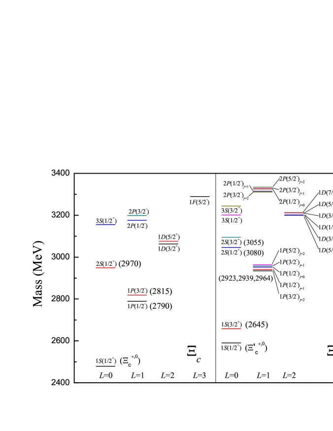
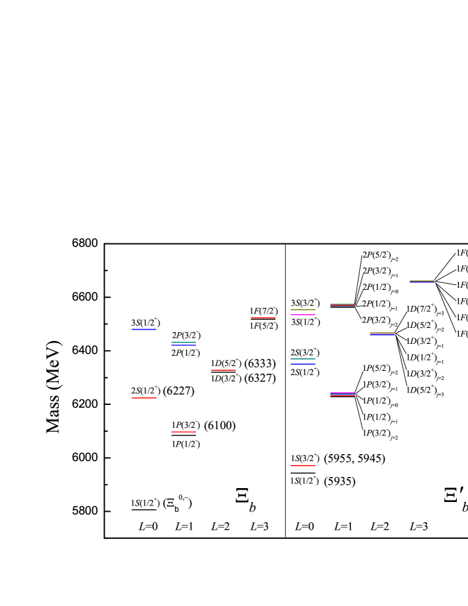
3.5 Shell structure of the mass spectra
The shell structure of the mass spectra are presented in Figs.10 and 11, where only the states with their root mean square radii less than 1 fm are collected. In this two figures, the well established baryons in experiment are labeled next to the corresponding states, and the recently observed baryons in experiment are arranged in their possible positions preliminarily according to the discussions in subsection 3.4.
From these two figures, we could get a bird’s-eye view of the mass spectra. Firstly, the baryon spectra of the () and () almost have the same shell structure. Secondly, the baryons with lighter masses were discovered earlier in experiment. Thirdly, there is a serious energy degeneracy in the , and states for the () family. And the calculated masses for the states of () family are very close to those of the states of the () family. This makes these states hard to be identified in experiment.
At last, the states which are possibly observed in experiment can be predicted. For the family, the doublets and the are likely to be experimentally observed first. In the family, the doublets might be the next ones to be observed. However, the predicted mass range of doublet states overlaps heavily with that of the states. As to the family, we find the state should have been discovered earlier in experiment and the predicted mass is MeV. The possibly observed states in the family should be the states where experimental observations will encounter the difficulty of the energy degeneracy.
IV. Conclusions
Motivated by the experimental development of singly heavy baryons, we investigate the strange single heavy baryon spectra in a three-quark system, where the relativistic quark model and the ISG method are employed. Considering the feature that the -mode appears lower in energy for definite states , we only focus on the -mode and obtain the mass spectra of the , , and families. For the well established baryons, our predicted masses can nicely reproduce the experimental data. We also investigate the root mean square radii and the radial probability density distributions, from which we can learn more about the structure of the strange single heavy baryons.
Based on the predicted mass spectra, we construct the Regge trajectories in the plane. Nevertheless, we can not currently construct the linear trajectories in the plane, which is an apparent difference between our mass spectra and those in the relativistic quark-diquark picture art1 .
For some recently observed baryons, We have preliminarily determined their reasonable positions in the mass spectra. At last, the mass spectral structure of the () and () families is presented, from which we could get a bird’s-eye view of the mass spectra and easily foresee where the experiment is going. Then, we analyze some states which might be observed in the forthcoming experiments.
Acknowledgements
Zhen-yu Li, one of the authors, thanks Wen-chao Dong for his valuable reference, helpful discussion and kind help in programming. And Li is also grateful to Professor Xian-Jian Shi for his support and encouragement. This work could not have been done without the joint efforts of all members of the phenomenological QCD theory group in North China Electric Power University. This research is supported by the Science and Technology Talent Project of Education Bureau of Guizhou Province, China (QJHKY [2018]058)), the National Natural Science Foundation of China (Grant No. 11675265), the Continuous Basic Scientific Research Project (Grant No. WDJC-2019-13), and the Leading Innovation Project (Grant No. LC 192209000701).
References
- (1) P. Avery, et al. [CLEO Collaboration], Phys. Rev. Lett. 75, 4364-4368 (1995), arXiv:hep-ex/9508010.
- (2) R. Mizuk, et al. [Belle Collaboration], Phys. Rev. Lett. 94, 122002 (2005), arXiv:hep-ex/0412069.
- (3) B. Aubert, et al. [BaBar Collaboration], arXiv:hep-ex/0607042.
- (4) R. Chistov, et al. [Belle Collaboration], Phys. Rev. Lett. 97, 162001 (2006), arXiv:hep-ex/0606051.
- (5) B. Aubert, et al. [BABAR Collaboration], Phys. Rev. D 77, 012002, (2008), arXiv:0710.5763 [hep-ex]
- (6) B. Aubert, et al. [BaBar Collaboration], Phys. Rev. Lett. 97, 232001 (2006), arXiv:hep-ex/0608055.
- (7) B. Aubert, et al. [BaBar Collaboration], Phys. Rev. Lett. 98, 012001 (2007), arXiv:hep-ex/0603052.
- (8) K. Abe, et al. [Belle Collaboration], Phys. Rev. Lett. 98, 262001 (2007), arXiv:hep-ex/0608043.
- (9) B. Aubert, et al. [BaBar Collaboration], Phys. Rev. D 77, 031101 (2008).
- (10) T. Lesiak, et al. [Belle Collaboration], Phys. Lett. B 665, 9 (2008), arXiv:0802.3968[hep-ex].
- (11) Y. Kato, et al. [Belle Collaboration], Phys. Rev. D 89, 052003 (2014), arXiv:1312.1026 [hep-ex].
- (12) E. Solovieva, et al., Phys. Lett. B 672, 1 (2009), arXiv:0808.3677 [hep-ex].
- (13) Y. B. Li, et al. [Belle Collaboration], Eur. Phys. J. C 78, 928 (2018), arXiv:1806.09182 [hep-ex].
- (14) R. Aaij, et al. [LHCb collaboration], Phys. Rev. Lett. 124, 222001 (2020), arXiv:2003.13649 [hep-ex].
- (15) T. J. Moon, et al. [Belle Collaboration], Phys. Rev. D 103, 111101 (2021), arXiv:2007.14700 [hep-ex].
- (16) Y. Kato, et al. [Belle Collaboration], Phys. Rev. D 94, 032002 (2016), arXiv:1605.09103 [hep-ex].
- (17) P. Abreu, et al. [DELPHI Collaboration], Z. Phys. C 68, 541 (1995).
- (18) V. Abazov, et al. [D0 Collaboration], Phys. Rev. Lett. 99, 052001 (2007), arXiv:0706.1690 [hep-ex].
- (19) T. Aaltonen, et al. [CDF Collaboration], Phys. Rev. Lett. 99, 052002 (2007), arXiv:0707.0589 [hep-ex].
- (20) T. Aaltonen [CDF Collaboration], Phys. Rev. Lett. 107, 102001 (2011), arXiv:1107.4015 [hep-ex].
- (21) CMS Collaboration, Phys. Rev. Lett 108, 252002 (2012), arXiv:1204.5955 [hep-ex].
- (22) R. Aaij, et al. [LHCb Collaboration], Phys. Rev. Lett. 114, 062004 (2015).
- (23) R. Aaij, et al. [LHCb Collaboration], J. High Energy Phys. 05, 161 (2016).
- (24) R. Aaij, et al. [LHCb Collaboration], Phys. Rev. Lett. 121, 072002 (2018), arXiv:1805.09418 [hep-ex].
- (25) R. Aaij, et al. [LHCb Collaboration], Phys. Rev. Lett. 121, 072002 (2018).
- (26) A. M. Sirunyan, et al. [CMS Collaboration], Phys. Rev. Lett. 126, 252003 (2021).
- (27) R. Aaij, et al. [LHCb collaboration], Phys. Rev. Lett. 128, 162001 (2022), arXiv:2110.04497 [hep-ex].
- (28) R. Aaij, et al. [LHCb Collaboration], Phys. Rev. Lett. 122, 012001 (2019), arXiv:1809.07752.
- (29) R. Aaij, et al. [LHCb Collaboration], Phys. Rev. Lett. 123, 152001 (2019).
- (30) P. A. Zyla, et al. [Particle Data Group], Prog. Theor. Exp. Phys. 083C01 (2020).
- (31) R.Chistov, et al. [Belle Collaboration], Phys. Rev. Lett. 97, 162001 (2006).
- (32) L. H. Liu, L. Y. Xiao, and X. H. Zhong, Phys. Rev. D 86, 034024 (2012), arXiv:1205.2943 [hep-ph].
- (33) D. D. Ye, Z. Zhao and A. Zhang, Phys. Rev. D 96, 114009 (2017), arXiv:1709.00689 [hep-ph].
- (34) Z. Zhao, D. D. Ye and A. Zhang, Phys. Rev. D 94, 114020 (2016).
- (35) Y. X. Yao, K. L. Wang and X. H. Zhong, Phys. Rev. D 98 076015 (2018), arXiv:1803.00364.
- (36) H. X. Chen, Q. Mao, A. Hosaka et al., Phys. Rev. D 94, 114016 (2016), arXiv:1611.02677v2 [hep-ph].
- (37) D. D. Ye, Z. Zhao and A. Zhang, Phys. Rev. D 96, 114003 (2017), arXiv:1710.10165 [hep-ph].
- (38) Z. G. Wang, Nucl. Phys. B 926, 467 (2018), arXiv:1705.07745 [hep-ph].
- (39) H. X. Chen and Q. Mao, Atsushi Hosaka et al. Phys. Rev. D 94, 114016 (2016), arXiv:1611.02677 [hep-ph].
- (40) B. Roelof, G. T. Hugo, G. Alessandro, et al., arXiv:2010.12437 [hep-ph].
- (41) K. L. Wang, Y. X. Yao, X. H. Zhong, et al., Phys. Rev. D 96, 116016 (2017). arXiv: hep-ph/1709.04268.
- (42) B. Chen, K. W. Wei and A. Zhang, Eur. Phys. J. A 51, 82 (2015), arXiv: hep-ph/1406.6561v4.
- (43) B. Chen, X. Liu and A. Zhang, Phys. Rev. D 95, 074022 (2017).
- (44) Z. G. Wang and H. J. Wang, Chin. Phys. C 45 013109 (2021) arXiv:2006.16776 [hep-ph].
- (45) J. Nieves, R. Pavao and L. Tolos, Eur. Phys. J. C 80, 22 (2020), arXiv:1911.06089 [hep-ph].
- (46) K. Gandhi and A. Kumar Rai, Eur. Phys. J. Plus 135, 213 (2020), arXiv:1911.11039 [hep-ph].
- (47) Z. Zhao, Phys. Rev. D 102, 096021 (2020), arXiv:2008.00630 [hep-ph].
- (48) B. Chen, K. W. Wei and A. Zhang, Eur. Phys. J. A 51, 82 (2015), arXiv:1406.6561 [hep-ph].
- (49) K. L. Wang, Q. F. Lü, and X. H. Zhong, Phys. Rev. D 99, 014011 (2019).
- (50) Y. Huang, C. J. Xiao, L. S. Geng et al., Phys. Rev. D 99, 014008 (2019).
- (51) B. Chen, K. W. Wei, X. Liu et al., Phys. Rev. D 98, 031502 (2018), arXiv:1805.10826 [hep-ph].
- (52) H. J. Wang, Z. Y. Di and Z. G. Wang, Int. J. Theor. Phys. 59(10): 3124-3133,(2020).
- (53) K. Azizi, Y. Sarac and H. Sundu, Journal of High Energy Physics 2021, 244 (2021), arXiv:2012.01086 [hep-ph].
- (54) G. L. Yu, Z. G. Wang and X. W. Wang, arXiv:2109.02217 [hep-ph].
- (55) H. M. Yang, H. X. Chen, E. L. Cui et al., arXiv:2205.07224 [hep-ph].
- (56) W. J. Wang, Y. H. Zhou, L. Y. Xiao, et al., Phys. Rev. D 105, 074008 (2022), arXiv:2202.05426 [hep-ph].
- (57) D. Ebert, R. N. Faustov and V. O. Galkin, Phys. Lett. B 659, 612 (2008), arXiv:0705.2957v2.
- (58) D. Ebert, R. N. Faustov and V. O. Galkin, Phys. Rev. D 84, 014025 (2011),
- (59) R. N. Faustov and V. O. Galkin, Phys. Rev. D 105, 014013 (2022), arXiv: hep-ph/2111.07702v1.
- (60) H. Mutuk, Eur. Phys. J. Plus 137:10 (2022), arXiv: hep-ph/2112.06205v1.
- (61) S. Capstick and N.Isgur, Phys. Rev. D 34, 2809 (1986).
- (62) T. Yoshida, E. Hiyama, A. Hosaka, et al., Phys. Rev. D 92, 114029 (2015). arXiv: hep-ph/1510.01067.
- (63) G. Yang, J. Ping, and J. Segovia, Few Body Syst. 59, 113 (2018). arXiv:1709.09315 [hep-ph].
- (64) G. Yang, J. Ping, P. G. Ortega, et al., Chinese Phys. C 44, 023102 (2020). arXiv:1904.10166 [hep-ph].
- (65) J. Segovia, D. R. Entem, F. Fernandez, et al., Int. J. Mod. Phys. E 22, 1330026 (2013). arXiv:1309.6926.
- (66) M. Q. Huang, Y. B. Dai and C. S. Huang, Phys. Rev. D 52, 3986 (1995); 55, 7317(E) (1997).
- (67) M. C. Banuls, A. Pich and I. Scimemi, Phys. Rev. D 61, 094009 (2000).
- (68) H. Y. Cheng and C. K. Chua, Phys. Rev. D 75, 014006 (2007).
- (69) N. Jiang, X. L. Chen and S. L. Zhu, Phys. Rev. D 92, 054017 (2015).
- (70) H. Y. Cheng and C. K. Chua, Phys. Rev. D 92, 074014 (2015).
- (71) X. H. Guo, K. W. Wei and X. H. Wu, Phys. Rev. D 77, 036003 (2008).
- (72) G. L. Yu, Z. G. Wang and Z. Y. Li, Chinese Physics C 39, 6, 063101 (2015), arXiv: hep-ph/1402.5955.
- (73) H. Z. He, W. Liang and Q. F. Lü, Phys. Rev. D 105, 014010 (2022), arXiv: hep-ph/2106.11045v2.
- (74) C. Chen, X. L. Chen, X. Liu et al., Phys. Rev. D 75, 094017 (2007).
- (75) P. Yang, J. J. Guo and A. Zhang, Phys. Rev. D 99, 034018 (2019), arXiv:1810.06947 [hep-ph].
- (76) J. J. Guo, P. Yang, and A. Zhang, Phys. Rev. D 100, 014001 (2019), arXiv:1902.07488 [hep-ph].
- (77) W. Liang, Q. F. Lü and X. H. Zhong, Phys. Rev. D 100, 054013 (2019).
- (78) Q. F. Lü and X. H. Zhong, Phys. Rev. D 101, 014017 (2020).
- (79) H. Z. He, W. Liang, Q. F. Lü et al., Sci. China Phys. Mech. Astron. 64, 261012(2021).
- (80) M. Padmanath, R. G. Edwards, N. Mathur et al., arXiv:1311.4806.
- (81) H. Bahtiyar, K. U. Can, G. Erkol et al., Phys. Lett. B 747, 281 (2015).
- (82) P. Perez-Rubio, S. Collins and G. S. Bali, Phys. Rev. D 92, 034504 (2015).
- (83) H. Bahtiyar, K. U. Can, G. Erkol et al., Phys. Lett. B 772, 121 (2017).
- (84) C. K. Chow, Phys. Rev. D 54, 3374 (1996).
- (85) S. L. Zhu and Y. B. Dai, Phys. Rev. D 59, 114015 (1999).
- (86) S. S. Agaev, K. Azizi and H. Sundu, Phys. Rev. D 96, 094011 (2017).
- (87) H. X. Chen, Q. Mao, W. Chen et al., Phys. Rev. D 95, 094008 (2017).
- (88) Z. G. Wang, Phys. Rev. D 81, 036002 (2010).
- (89) Z. G. Wang, Eur. Phys. J. A 44, 105 (2010).
- (90) T. M. Aliev, K. Azizi and H. Sundu, Eur. Phys. J. C 75, 14 (2015).
- (91) T. M. Aliev, K. Azizi and A. Ozpineci, Phys. Rev. D 79, 056005 (2009).
- (92) T. M. Aliev, T. Barakat and M. Savc, Phys. Rev. D 93, 056007 (2016).
- (93) T. M. Aliev, K. Azizi and M. Savci, Phys. Lett. B 696, 220(2011).
- (94) T. M. Aliev, K. Azizi, Y. Sarac et al., Phys. Rev. D 99, 094003 (2019).
- (95) S. L. Zhu, Phys. Rev. D 61, 114019 (2000).
- (96) Z. G. Wang, Eur. Phys. J. A 47, 81 (2011).
- (97) Q. Mao, H. X. Chen, W. Chen et al., Phys. Rev. D 92, 114007 (2015), arXiv:1510.05267 [hep-ph].
- (98) H. X. Chen, Q. Mao, A. Hosaka et al., Phys. Rev. D 94, 114016 (2016).
- (99) Q. Mao, H. X. Chen, A. Hosaka et al., Phys. Rev. D 96, 074021 (2017).
- (100) T. M. Aliev, K. Azizi, Y. Sarac et al., Phys. Rev. D 98, 094014 (2018).
- (101) E. L. Cui, H. M. Yang, H. X. Chen et al., Phys.Rev. D 99, 094021 (2019).
- (102) K. Azizi, Y. Sarac and H. Sundu, Phys. Rev. D 101, 074026 (2020).
- (103) K. Azizi, Y. Sarac and H. Sundu, Phys. Rev. D 102, 034007 (2020).
- (104) Z. G. Wang, Eur. Phys. J. C, 75(8), 359 (2015).
- (105) S. Godfrey and N. Isgur, Phys. Rev. D 32, 189 (1985).
- (106) E. Hiyama, Y. Kino and M. Kamimura, Prog. Part. Nucl. Phys. 51, 223 (2003).
- (107) Q. F. Lü, D. Y. Chen and Y. B. Dong, Phys. Rev. D 102, 034012 (2020).
- (108) Q. F. Lü, D. Y. Chen and Y. B. Dong, Eur. Phys. J. C 80, 871 (2020).
- (109) Q. F. Lü, D. Y. Chen and Y. B. Dong, Phys. Rev. D 102, 074021 (2020).
- (110) E. Hiyama, A. Hosaka, M. Oka et al., Phys. Rev. C 98, 045208 (2018), arXiv:1803.11369v1 [nucl-th].
- (111) H. X. Chen, W. Chen, X. Liu, et al. Physics Reports 639,1-121(2016), arXiv:1601.02092 [hep-ph].
- (112) F. K. Guo, C. Hanhart, U. G. Meiner, et al., Rev. Mod. Phys. 90,015004(2018), arXiv:1705.00141 [hep-ph].
- (113) R. Aaij, et al.,[LHCb collaboration], Phys. Rev. Lett. 122,222001(2019), arXiv:1904.03947 [hep-ex].
- (114) X. K. Dong, F. K. Guo, B. S. Zou,Commun. Theor. Phys. 73(2021)125201, arXiv:2108.02673 [hep-ph].
- (115) T. Ji, X. K. Dong, F. K. Guo, et al.,Phys. Rev. Lett. 129,102002(2022), arXiv:2205.10994 [hep-ph].
- (116) C. Q. Pang, J. Z. Wang, X. Liu et al., Eur. Phys. J. C 77, 861 (2017).
- (117) H. Georgi, Physics Letters B 240, 447450, (1990).
- (118) B. Chen, S. Q. Luo, X. Liu et al., Phys. Rev. D 100, 094032 (2019), arXiv:1910.03318.
- (119) H. X. Chen, W. Chen, X. Liu et al., Rept. Prog. Phys. 80, 7, 076201 (2017), arXiv:1609.08928,
- (120) H. Garcilazo, J. Vijande and A. Valcarce, J. phys. G 34, 961(2007).
- (121) S. Migura, D. Merten, B. Metsch et al., Eur. Phys. J. A 28, 41 (2006).
- (122) A. Martin, Z. Phys. C 32, 359 (1986).
- (123) T. Regge, Nuovo Cim. 14, 951 (1959).
- (124) T. Regge, Nuovo Cim. 18, 947956 (1960).
- (125) G. F. Chew and S. C. Frautschi, Phys. Rev. Lett. 7, 394397 (1961) .
- (126) G. F. Chew and S. C. Frautschi, Phys. Rev. Lett. 8, 4144 (1962).
- (127) M. Baker and R. Steinke, Phys. Rev. D 65, 094042 (2002).
- (128) P. D. B. Collins, An Introduction to Regge Theory and High Energy Physics (Cambridge University Press),Cambridge, England, 1977.
Appendix
| () | mass | exp.art2 | art1 | |||||
|---|---|---|---|---|---|---|---|---|
| 0 0 0 0 0 | () | 0.512 | 0.437 | 2479 |
|
2476 | ||
| () | 0.645 | 0.768 | 2949 | 2970? | 2959 | |||
| () | 0.968 | 0.607 | 3155 | 3123?art31 | 3323 | |||
| () | 0.690 | 1.131 | 3318 | 3632 | ||||
| 0 1 1 0 1 | () | 0.542 | 0.627 | 2789 |
|
2792 | ||
| () | 0.615 | 0.948 | 3176 | 3179 | ||||
| () | 1.038 | 0.763 | 3390 | 3500 | ||||
| () | 0.655 | 1.285 | 3492 | 3785 | ||||
| 0 1 1 0 1 | () | 0.550 | 0.654 | 2819 |
|
2819 | ||
| () | 0.613 | 0.977 | 3199 | 3201 | ||||
| () | 1.053 | 0.779 | 3412 | 3519 | ||||
| () | 0.645 | 1.278 | 3508 | 3804 | ||||
| 0 2 2 0 2 | () | 0.561 | 0.825 | 3063 | 3055? | 3059 | ||
| () | 0.601 | 1.161 | 3406 | 3388 | ||||
| () | 1.084 | 0.936 | 3617 | 3678 | ||||
| () | 0.627 | 1.349 | 3676 | 3945 | ||||
| 0 2 2 0 2 | () | 0.565 | 0.843 | 3076 | 3080? | 3076 | ||
| () | 0.604 | 1.190 | 3419 | 3407 | ||||
| () | 1.092 | 0.945 | 3627 | 3699 | ||||
| () | 0.618 | 1.328 | 3688 | 3965 | ||||
| 0 3 3 0 3 | () | 0.567 | 0.998 | 3289 | 3278 | |||
| () | 0.604 | 1.413 | 3613 | 3572 | ||||
| () | 1.103 | 1.087 | 3817 | 3845 | ||||
| () | 0.602 | 1.314 | 3861 | 4098 | ||||
| 0 3 3 0 3 | () | 0.569 | 1.009 | 3294 | 3292 | |||
| () | 0.607 | 1.439 | 3619 | 3592 | ||||
| () | 1.111 | 1.088 | 3821 | 3865 | ||||
| () | 0.589 | 1.290 | 3871 | 4120 | ||||
| 0 4 4 0 4 | () | 0.566 | 1.147 | 3486 | 3469 | |||
| () | 0.612 | 1.676 | 3798 | 3745 | ||||
| () | 1.121 | 1.205 | 4000 | |||||
| () | 0.559 | 1.222 | 4054 | |||||
| 0 4 4 0 4 | () | 0.567 | 1.154 | 3487 | 3483 | |||
| () | 0.613 | 1.692 | 3799 | 3763 | ||||
| () | 1.126 | 1.208 | 4001 | |||||
| () | 0.551 | 1.202 | 4064 |
| () | mass | exp.art2 | art1 | |||||
|---|---|---|---|---|---|---|---|---|
| 0 0 0 1 1 | () | 0.590 | 0.431 | 2590 |
|
2579 | ||
| () | 0.821 | 0.705 | 3046 | 3055? | 2983 | |||
| () | 0.918 | 0.671 | 3201 | 3377 | ||||
| () | 0.897 | 1.053 | 3425 | 3695 | ||||
| 0 0 0 1 1 | () | 0.611 | 0.476 | 2658 |
|
2654 | ||
| () | 0.801 | 0.763 | 3095 | 3080? | 3026 | |||
| () | 0.968 | 0.676 | 3244 | 3396 | ||||
| () | 0.850 | 1.095 | 3456 | 3709 | ||||
| 0 1 1 1 0 | () | 0.649 | 0.671 | 2952 | 2936 | |||
| () | 0.762 | 0.978 | 3326 | 3313 | ||||
| () | 1.055 | 0.811 | 3469 | 3630 | ||||
| () | 0.783 | 1.245 | 3636 | 3912 | ||||
| 0 1 1 1 1 | () | 0.644 | 0.659 | 2941 | 2854 | |||
| () | 0.763 | 0.962 | 3315 | 3267 | ||||
| () | 1.048 | 0.804 | 3460 | 3598 | ||||
| () | 0.788 | 1.248 | 3628 | 3887 | ||||
| 0 1 1 1 1 | () | 0.651 | 0.677 | 2958 | 2935 | |||
| () | 0.761 | 0.985 | 3331 | 3311 | ||||
| () | 1.059 | 0.814 | 3473 | 3628 | ||||
| () | 0.780 | 1.243 | 3640 | 3911 | ||||
| 0 1 1 1 2 | () | 0.642 | 0.653 | 2934 | 2930?art120 | 2912 | ||
| () | 0.764 | 0.955 | 3310 | 3293 | ||||
| () | 1.043 | 0.801 | 3456 | 3613 | ||||
| () | 0.791 | 1.249 | 3624 | 3898 | ||||
| 0 1 1 1 2 | () | 0.652 | 0.682 | 2964 | 2929 | |||
| () | 0.761 | 0.993 | 3335 | 3303 | ||||
| () | 1.062 | 0.817 | 3477 | 3619 | ||||
| () | 0.778 | 1.241 | 3644 | 3902 | ||||
| 0 2 2 1 1 | () | 0.668 | 0.851 | 3201 | 3163 | |||
| () | 0.744 | 1.195 | 3541 | 3505 | ||||
| () | 1.104 | 0.955 | 3676 | |||||
| () | 0.738 | 1.303 | 3816 | |||||
| 0 2 2 1 1 | () | 0.671 | 0.865 | 3211 | 3167 | |||
| () | 0.745 | 1.219 | 3550 | 3506 | ||||
| () | 1.111 | 0.963 | 3684 | |||||
| () | 0.734 | 1.285 | 3827 |
| () | mass | art1 | |||
|---|---|---|---|---|---|
| 0 2 2 1 2 | () | 0.668 | 0.851 | 3201 | 3160 |
| () | 0.744 | 1.195 | 3541 | 3497 | |
| () | 1.104 | 0.955 | 3676 | ||
| () | 0.738 | 1.303 | 3816 | ||
| 0 2 2 1 2 | () | 0.671 | 0.865 | 3211 | 3166 |
| () | 0.745 | 1.219 | 3551 | 3504 | |
| () | 1.111 | 0.963 | 3685 | ||
| () | 0.734 | 1.285 | 3828 | ||
| 0 2 2 1 3 | () | 0.667 | 0.850 | 3200 | 3153 |
| () | 0.744 | 1.193 | 3540 | 3493 | |
| () | 1.104 | 0.954 | 3676 | ||
| () | 0.738 | 1.304 | 3815 | ||
| 0 2 2 1 3 | () | 0.672 | 0.868 | 3213 | 3147 |
| () | 0.746 | 1.224 | 3552 | 3486 | |
| () | 1.112 | 0.965 | 3686 | ||
| () | 0.733 | 1.281 | 3829 | ||
| 0 3 3 1 2 | () | 0.676 | 1.022 | 3424 | 3418 |
| () | 0.742 | 1.454 | 3744 | ||
| () | 1.136 | 1.096 | 3872 | ||
| () | 0.699 | 1.262 | 4010 | ||
| 0 3 3 1 2 | () | 0.678 | 1.031 | 3428 | 3408 |
| () | 0.744 | 1.474 | 3748 | ||
| () | 1.140 | 1.101 | 3876 | ||
| () | 0.698 | 1.243 | 4020 | ||
| 0 3 3 1 3 | () | 0.676 | 1.022 | 3424 | 3394 |
| () | 0.742 | 1.454 | 3744 | ||
| () | 1.136 | 1.096 | 3872 | ||
| () | 0.699 | 1.263 | 4009 | ||
| 0 3 3 1 3 | () | 0.678 | 1.031 | 3428 | 3393 |
| () | 0.744 | 1.475 | 3748 | ||
| () | 1.140 | 1.101 | 3876 | ||
| () | 0.698 | 1.242 | 4021 | ||
| 0 3 3 1 4 | () | 0.676 | 1.021 | 3423 | 3373 |
| () | 0.742 | 1.453 | 3744 | ||
| () | 1.136 | 1.095 | 3872 | ||
| () | 0.699 | 1.264 | 4009 | ||
| 0 3 3 1 4 | () | 0.678 | 1.032 | 3428 | 3357 |
| () | 0.744 | 1.476 | 3749 | ||
| () | 1.140 | 1.102 | 3876 | ||
| () | 0.698 | 1.241 | 4021 |
| () | mass | exp.art2 | art1 | |||||
|---|---|---|---|---|---|---|---|---|
| 0 0 0 0 0 | () | 0.518 | 0.400 | 5806 |
|
5803 | ||
| () | 0.607 | 0.705 | 6224 | 6266 | ||||
| () | 0.990 | 0.549 | 6480 | 6601 | ||||
| () | 0.672 | 1.066 | 6568 | 6913 | ||||
| 0 1 1 0 1 | () | 0.539 | 0.571 | 6084 | 6120 | |||
| () | 0.586 | 0.844 | 6421 | 6496 | ||||
| () | 1.034 | 0.713 | 6690 | 6805 | ||||
| () | 0.673 | 1.281 | 6732 | 7068 | ||||
| 0 1 1 0 1 | () | 0.543 | 0.583 | 6097 | 6100.3(0.6) | 6130 | ||
| () | 0.585 | 0.853 | 6432 | 6502 | ||||
| () | 1.043 | 0.719 | 6700 | 6810 | ||||
| () | 0.668 | 1.293 | 6739 | 7073 | ||||
| 0 2 2 0 2 | () | 0.551 | 0.743 | 6320 | 6366 | |||
| () | 0.568 | 0.962 | 6613 | 6690 | ||||
| () | 0.990 | 1.040 | 6883 | 6966 | ||||
| () | 0.778 | 1.359 | 6890 | 7208 | ||||
| 0 2 2 0 2 | () | 0.553 | 0.751 | 6327 | 6373 | |||
| () | 0.568 | 0.967 | 6621 | 6696 | ||||
| () | 0.948 | 1.124 | 6888 | 6970 | ||||
| () | 0.831 | 1.294 | 6894 | 7212 | ||||
| 0 3 3 0 3 | () | 0.555 | 0.903 | 6518 | 6577 | |||
| () | 0.553 | 1.064 | 6795 | 6863 | ||||
| () | 0.619 | 1.646 | 7032 | 7114 | ||||
| () | 1.110 | 0.960 | 7057 | 7339 | ||||
| 0 3 3 0 3 | () | 0.556 | 0.909 | 6523 | 6581 | |||
| () | 0.553 | 1.070 | 6801 | 6867 | ||||
| () | 0.618 | 1.641 | 7034 | 7117 | ||||
| () | 1.111 | 0.965 | 7060 | 7342 | ||||
| 0 4 4 0 4 | () | 0.554 | 1.048 | 6692 | 6760 | |||
| () | 0.542 | 1.178 | 6970 | 7020 | ||||
| () | 0.607 | 1.745 | 7167 | |||||
| () | 1.119 | 1.095 | 7214 | |||||
| 0 4 4 0 4 | () | 0.555 | 1.052 | 6695 | 6762 | |||
| () | 0.544 | 1.189 | 6975 | 7032 | ||||
| () | 0.605 | 1.737 | 7169 | |||||
| () | 1.120 | 1.098 | 7217 |
| () | mass | exp.art2 | art1 | |||||
|---|---|---|---|---|---|---|---|---|
| 0 0 0 1 1 | () | 0.604 | 0.411 | 5943 | 5935.02(0.05) | 5936 | ||
| () | 0.741 | 0.697 | 6350 | 6329 | ||||
| () | 0.998 | 0.559 | 6535 | 6687 | ||||
| () | 0.804 | 1.063 | 6691 | 6978 | ||||
| 0 0 0 1 1 | () | 0.614 | 0.431 | 5971 |
|
5963 | ||
| () | 0.735 | 0.716 | 6370 | 6342 | ||||
| () | 1.017 | 0.566 | 6554 | 6695 | ||||
| () | 0.793 | 1.087 | 6705 | 6984 | ||||
| 0 1 1 1 0 | () | 0.642 | 0.608 | 6238 | 6233 | |||
| () | 0.709 | 0.866 | 6569 | 6611 | ||||
| () | 1.074 | 0.705 | 6758 | 6915 | ||||
| () | 0.772 | 1.296 | 6866 | 7174 | ||||
| 0 1 1 1 1 | () | 0.640 | 0.603 | 6232 | 6227 | |||
| () | 0.709 | 0.862 | 6564 | 6604 | ||||
| () | 1.071 | 0.701 | 6754 | 6904 | ||||
| () | 0.774 | 1.292 | 6863 | 7164 | ||||
| 0 1 1 1 1 | () | 0.643 | 0.610 | 6240 | 6234 | |||
| () | 0.709 | 0.868 | 6572 | 6605 | ||||
| () | 1.076 | 0.707 | 6760 | 6905 | ||||
| () | 0.771 | 1.297 | 6868 | 7163 | ||||
| 0 1 1 1 2 | () | 0.639 | 0.600 | 6229 |
|
6224 | ||
| () | 0.709 | 0.859 | 6562 | 6598 | ||||
| () | 1.069 | 0.700 | 6752 | 6900 | ||||
| () | 0.774 | 1.291 | 6861 | 7159 | ||||
| 0 1 1 1 2 | () | 0.644 | 0.613 | 6243 | 6226 | |||
| () | 0.708 | 0.871 | 6574 | 6596 | ||||
| () | 1.077 | 0.708 | 6762 | 6897 | ||||
| () | 0.770 | 1.299 | 6869 | 7156 | ||||
| 0 2 2 1 1 | () | 0.656 | 0.773 | 6460 | 6447 | |||
| () | 0.690 | 0.992 | 6757 | 6767 | ||||
| () | 1.109 | 0.845 | 6941 | |||||
| () | 0.754 | 1.464 | 7017 | |||||
| 0 2 2 1 1 | () | 0.658 | 0.780 | 6466 | 6459 | |||
| () | 0.690 | 0.998 | 6763 | 6775 | ||||
| () | 1.111 | 0.850 | 6946 | |||||
| () | 0.751 | 1.462 | 7020 |
| () | mass | art1 | |||
|---|---|---|---|---|---|
| 0 2 2 1 2 | () | 0.656 | 0.773 | 6460 | 6431 |
| () | 0.690 | 0.992 | 6758 | 6751 | |
| () | 1.109 | 0.845 | 6941 | ||
| () | 0.754 | 1.464 | 7017 | ||
| 0 2 2 1 2 | () | 0.658 | 0.780 | 6466 | 6432 |
| () | 0.690 | 0.999 | 6764 | 6751 | |
| () | 1.112 | 0.851 | 6946 | ||
| () | 0.751 | 1.462 | 7021 | ||
| 0 2 2 1 3 | () | 0.656 | 0.773 | 6460 | 6420 |
| () | 0.690 | 0.991 | 6757 | 6740 | |
| () | 1.108 | 0.844 | 6941 | ||
| () | 0.754 | 1.464 | 7017 | ||
| 0 2 2 1 3 | () | 0.658 | 0.781 | 6467 | 6414 |
| () | 0.690 | 1.000 | 6765 | 6736 | |
| () | 1.112 | 0.851 | 6946 | ||
| () | 0.751 | 1.461 | 7021 | ||
| 0 3 3 1 2 | () | 0.663 | 0.931 | 6657 | 6675 |
| () | 0.678 | 1.121 | 6942 | ||
| () | 1.130 | 0.986 | 7110 | ||
| () | 0.734 | 1.580 | 7162 | ||
| 0 3 3 1 2 | () | 0.664 | 0.936 | 6660 | 6686 |
| () | 0.680 | 1.130 | 6946 | ||
| () | 1.131 | 0.991 | 7114 | ||
| () | 0.732 | 1.573 | 7164 | ||
| 0 3 3 1 3 | () | 0.663 | 0.931 | 6657 | 6640 |
| () | 0.678 | 1.121 | 6942 | ||
| () | 1.130 | 0.986 | 7110 | ||
| () | 0.734 | 1.580 | 7162 | ||
| 0 3 3 1 3 | () | 0.664 | 0.936 | 6660 | 6641 |
| () | 0.680 | 1.131 | 6947 | ||
| () | 1.131 | 0.991 | 7114 | ||
| () | 0.731 | 1.572 | 7165 | ||
| 0 3 3 1 4 | () | 0.663 | 0.931 | 6657 | 6619 |
| () | 0.678 | 1.121 | 6942 | ||
| () | 1.130 | 0.986 | 7110 | ||
| () | 0.734 | 1.580 | 7162 | ||
| 0 3 3 1 4 | () | 0.664 | 0.937 | 6661 | 6610 |
| () | 0.680 | 1.132 | 6947 | ||
| () | 1.131 | 0.991 | 7114 | ||
| () | 0.731 | 1.572 | 7165 |
| Trajectory | ||||||
|---|---|---|---|---|---|---|
| (GeV2) | (GeV2) | (GeV2) | (GeV2) | (GeV2) | (GeV2) | |
| Trajectory | ||||||
|---|---|---|---|---|---|---|
| (GeV2) | (GeV2) | (GeV2) | (GeV2) | (GeV2) | (GeV2) | |