Tailored particle current in an optical lattice by a weak time-symmetric harmonic potential

Brownian motors or ratchets are spatially periodic systems with noise and/or dissipation in which a directed current of particles can emerge from an unbiased zero-mean external force Reimann_2002 ; Hanggi_Marchesoni_2009 . Models for biological engines that transform chemical energy into unidirectional mechanical motion behave as Brownian motors Julicher_1997 . Extensive studies of the ratchet effect in classical systems Schanz2001 stated the relation between symmetry breaking potentials and the existence of the asymptotic current Flach_2000 . For a system driven by a flashing potential of the form $V(x,t)=V_{x}(x)V_{t}(t)$ with $V_{t}(t)=V_{t}(t+T)$ of zero mean and $V_{x}(x)=V_{x}(x+L_{x})$ there are up to four different symmetries in the classical system that must be broken in order to generate an asymptotic current Denisov2007 . A ratchet current arises if one breaks the relevant spatio-temporal symmetries, here denoted by $S_{x}$, and the time-reversal symmetry $S_{t}:(x,p,t)\rightarrow(x,-p,-t+2t_{s})$. Lately there has been an increasing interest in the coherent ratchet effect in Hamiltonian quantum systems Reimann_Grifoni_Hanggi_2002 . It has been shown that the same symmetry requirements apply to them Denisov2007 , i.e. if the Hamiltonian preserves any of the symmetries, no asymptotic current is possible.

Experimentally, directed current generation was first studied in solid state devices, quantum dots and Josephson junctions Solidstate . More recently, the precise control achievable in cold atom experiments opened up the possibility of realizing directed atomic currents for Hamiltonian systems with controllable or no dissipation in the time scale of the measurements Schiavoni2003 ; Gommers2005 ; Jones_2007 ; QAM . Recently, a very clean realization of a coherent quantum ratchet was experimentally demonstrated in a Bose-Einstein condensate exposed to a sawtooth potential realized with an optical lattice which was periodically modulated in time Salger_2009 . Directed transport of atoms was observed when the driving lattice potential broke the spatio-temporal symmetries. The current oscillations and the dependence of the current on the initial time and the resonant frequencies Res_2007 were measured, demonstrating the quantum character of the ratchet.

Although the generation of an asymptotic directed current needs the breaking of the symmetries $S_{x}$ and $S_{t}$ simultaneously for unbiased potentials, there has been a recent discussion on the possibility of obtaining long-lasting directed currents without it Hanggi2009 ; Sols ; comment ; reply ; Moskalets . Many-body effects Hanggi2009 ; Moskalets with the proper choice of the initial state Hanggi2009 or an accidental degeneracy in the quasienergy spectrum reply may result in a directed current without breaking the time-reversal symmetry. In contrast to previous works we show here that one can exploit a quasi-degeneracy, present for a wide range of parameters, in the quasienergy spectrum in order to generate a long-lasting directed average current in a weakly driven system where we can achieve full control over its magnitude and time scale.
Previous work on quantum accelerators QAM has shown that in the presence of quantum resonances one can obtain large currents without breaking the time-reversal symmetry using a delta-kicked potential in time. Essentially, for particular values of the Hamiltonian parameters the spectrum of the Floquet operator becomes continuous due to quantum resonances. Under such circumstances one can obtain a linear increase in momentum with time which has been claimed as a true ratchet effect driven by resonances instead of noise QAM2 . However, there is no formal proof that the dynamics show unbounded acceleration for times longer that those that are computed QAM . Nonetheless, a significant difference between quantum accelerator ratchets and our system is the existence of a constant component in the delta potential.

One useful way of treating time-periodic quantum Hamiltonians, $H(t)=H(t+T)$, is the Floquet formalism Floquet . The cyclic states $\left|\,\phi_{j}(t+T)\right\rangle=e^{-i\varepsilon_{j}T}\left|\,\phi_{j}(t)\right\rangle$ are the eigenstates of the evolution operator for one period while the quasienergies $\varepsilon_{j}$ are the eigenvalues. The solution to the time-dependent Schrödinger equation $H(t)\left|\,\psi(t)\right\rangle=i\hbar{\partial}\left|\,\psi(t)\right\rangle/{\partial t}$ can be spanned in the cyclic eigenbasis ($\hbar=1$)

where $c_{j}=\langle\phi_{j}(0)|\psi(0)\rangle$. The average current generated during $n$ cycles is given by $\mathcal{I}(t=nT)=\frac{1}{n}\sum_{m=1}^{n}\mathcal{I}_{m}$ with

where $p$ is the momentum operator. Note that due to the periodicity of the cyclic states the average current during $n$ cycles can be simplified in terms of integrals of the cyclic states during the first period

which is valid for a discrete Floquet spectrum and where $\ \langle p\rangle_{jj^{\prime}}:=\frac{1}{T}\int_{0}^{T}\left\langle\phi_{j}(t)\,\right|p\left|\,\phi_{j^{\prime}}(t)\right\rangle e^{-it(\varepsilon_{j^{\prime}}-\varepsilon_{j})}dt$. Our model, that represents well optical lattices, has by construction a pure point spectrum. In the limit of an infinite number of states the single-band tight-binding model remains integrable spectrum1 . However, if more bands are added the spectrum could become absolutely continuous (in resonance) or singular continuous. Our guess, based on our previous experience in related problems spectrum2 , is that except at very long times even if the spectrum is singular continuous the time evolution will be similar to that given by a pure point spectrum. In general, a sum of oscillatory off-diagonal terms with arbitrary exponents decays rapidly decay and for long times only the diagonal terms in Eq. (3) remain. If both $S_{x}$ and $S_{t}$ are broken, the cyclic eigenstates desymmetrise and carry net momentum, i.e. $\langle p\rangle_{jj}\neq 0$ Denisov2007 . In such case, the asymptotic average current at $n\rightarrow\infty$ is nonzero $\mathcal{I}(\infty)=\sum_{j}|c_{j}|^{2}\langle p\rangle_{jj}$. Correspondingly, if either of the relevant symmetries is not broken $\langle p\rangle_{jj}=0$ and thus $\mathcal{I}(\infty)=0$. Note, however, that the off-diagonal terms in Eq. (3) become relevant if the initial state projects mainly into degenerate or quasidegenerate cyclic states with $\langle p\rangle_{jj^{\prime}}\neq 0$. If one induces a resonance between the proper quasienergy states at low driving, the average current contains only a small number of terms in the sum and the exponents can be very small, leading to very slow oscillations whose period can be fitted by tunning the driving. In order to maximise the average current one should then optimise both the projection into the initial states $c_{j}c^{*}_{j^{\prime}}$ and the $\langle p\rangle_{jj^{\prime}}$. We illustrate this here and show that it is possible to populate a high average momentum superposition of cyclic eigenstates for times which can be tuned up to the lifetime of the experiment.

We consider a driven system of non-interacting bosons with $H(t)=H_{0}+V(t)$ in a lattice of $L$ sites with periodic boundary conditions lattice and

with $M$ integer, where $J$ is the tunneling probability and $\left|\,l\right\rangle$ represents the state of a boson located on site $l$. The eigenenergies of $H_{0}$ are $E_{k}=-2J\cos(2\pi k/L)$ with integer $k=\left[-k_{\rm max},k_{\rm max}\right]$ where $k_{\rm max}=(L-1)/2$ for $L$ odd and the corresponding momentum eigenvectors $\langle l\left|\,k\right\rangle=e^{i\frac{k2\pi l}{L}}/\sqrt{L}$ are degenerate for $\pm k$. For convenience one can introduce the basis $\langle l\left|\,s_{k}\right\rangle=\sqrt{2/L}\cos(k2\pi l/L)$ and $\langle l\left|\,a_{k}\right\rangle=\sqrt{2/L}\sin(k2\pi l/L)$ which are symmetric or antisymmetric under the inversion of $k$. We add a time and spatially modulated periodic function $V(l,t)$ with frequency $\omega=2\pi/T$ tuned to the $M$-dependent resonant condition Sols ; creff_sols2

and consider the zero momentum $\left|\,0\right\rangle$ as initial state. Note that in contrast to Sols ; creff_sols2 we add the parameters $M$ and $\phi$ to the driving potential in Eq.(5). Parameter $M\leq k_{\rm max}/2$ allows for the coupling of the initial state to very high momentum states $\left|\,M\right\rangle$ and $\left|\,2M\right\rangle$, and the parameter $\phi$, key to our model, allows for the coupling between the $\left|\,s_{k}\right\rangle$ and $\left|\,a_{k}\right\rangle$ basis states.

Our choice of a two-harmonic spatial potential times a monochromatic time-dependent potential implies that symmetry $S_{t}$ (labelled $S_{2}$ in Denisov2007 ) is not broken for $t_{s}=\pi/(2\omega)$. Therefore $\langle p\rangle_{jj}=0$ and no asymptotic current is possible for our system. The average current generated after $n$ cycles arises only from crossed terms between the cyclic states. Our aim is to maximise the average current during any experimental time $t_{e}$. The key ingredients are to keep few terms in the sum in Eq.(3), with small exponents and relevant prefactors. The two first are achieved by tuning the resonance in Eq. (6) with weak driving $V/J<1$. We show that the prefactors can be successfully optimized if the quasiresonant cyclic states that have non-zero projection into the initial zero momentum state mix the symmetric and antisymmetric momentum states, which is obtained for $\phi\neq l\frac{\pi}{2}$ for $l$ integer. For $\phi=l\pi$, accidental degeneracies could in principle allow to obtain a small non asymptotic current for some specific parameters and a particular value of the coupling reply . In contrast, we show that for $\phi\neq l\pi/2$ one can tailor an interference between two paths of the same perturbative order and find optimal parameters $M$, $\phi$ and $\alpha$ for any $L$ and $J$ set by $H_{0}$, to obtain an average current that can be tuned up to near optimal value $\mathcal{I}(t_{e})\simeq M\simeq k_{\rm max}/4$, for a time interval $[0,t_{e}]$ where $t_{e}$ can be independently tuned by adjusting the driving strength $V/J$.

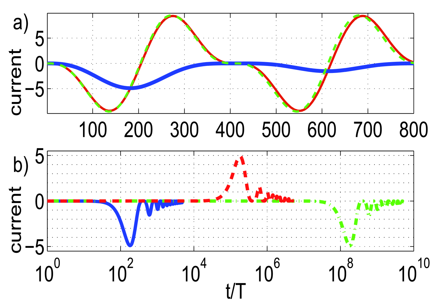
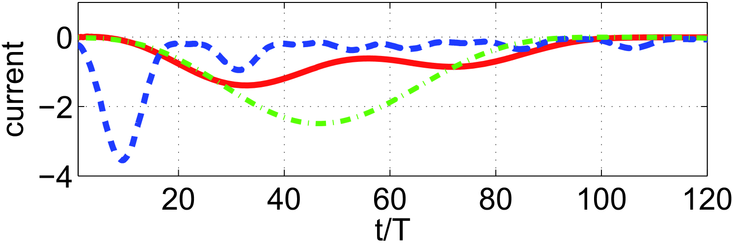
We show in fig 1a) the average current $\mathcal{I}$ and the oscillating average current per cycle $\mathcal{I}_{m}$ as a function of the number of cycles. We note that the average current achieves a maximum $M$ in recoil units and, as expected, vanishes for long times. We observe in fig 1b) that the current changes direction with a sign change in $\phi$ and $t_{e}$ scales with $V^{-2}\omega$. For the weak driving strength used here the current is nearly zero ($\mathcal{I}\leq 10^{-3}$) for $\phi=0$.

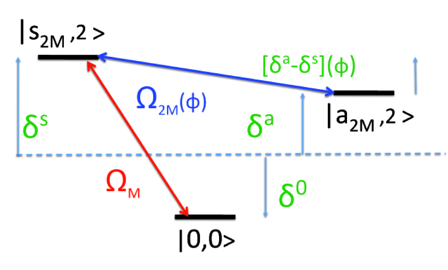
The previous results are obtained from a full numerical calculation. In order to further understand the effect we follow the methodology of creff_sols2 and develop an approximate perturbative model. We find that for our potential this simplified model also explains the main features and gives very accurate results for low driving. Close to the resonance Eq. (6) and for weak driving $V/J<1$ the dynamics of the system involve only three Floquet basis states $\{\left|\,s_{2M},2\right\rangle,\left|\,0,0\right\rangle,\left|\,a_{2M},2\right\rangle\}$, where $\left|\,j\right\rangle=\left|\,k,n\right\rangle$ with $\langle t\left|\,n\right\rangle=e^{-in\omega t}$. We apply time-independent perturbation theory in Floquet space, using the $\mathcal{T}$-matrix approach $\mathcal{T}(\epsilon)=V+VG_{0}(\epsilon)\mathcal{T}$ tmatrix , where $G_{0}(\epsilon)=\sum_{j}\frac{\left|\,j\right\rangle\left\langle j\,\right|}{\epsilon-\varepsilon^{0}_{j}}$ and $\varepsilon^{0}_{j}\equiv E_{k}-n\omega$. Around the ground state quasienergy $\epsilon=\varepsilon^{0}_{0}$, the first non-zero term connecting the three states is given by the second order in the expansion $\mathcal{T}(\varepsilon^{0}_{0})\simeq VG_{0}(\varepsilon^{0}_{0})V$ which reduces to

A sketch of the relevant processes is depicted in Fig.2 and the exact values of the matrix elements, inverse of quasienergy differences which depend on $M/L$, can be found in the complementary material. The energy shifts are $\delta$ and the couplings $\Omega$ that correspond to each part of the potential in Eq. (5) are indicated by the subindex $M$ or $2M$. Remarkably, $\Omega_{2M}\propto\alpha^{2}\sin(2\phi)$ and thus the coupling between the symmetric and antisymmetric basis states requires $\phi\neq 0$. The other effect of $\phi$ is to bring those states closer in energy $\delta^{s}-\delta^{a}\propto\alpha^{2}\cos(2\phi)$. The optimal current is obtained when the cyclic states (related to eigenvectors of the above matrix) mix the three basis states on an equal foot, corresponding to the two second order processes sketched in Fig. 2 being of the same order. Due to the structure of the spectrum, this optimal mixing can be reached for $M\leq k_{\rm max}/4$. Then all the matrix elements in Eq. (10) are of order $\mathcal{O}\simeq 1/\omega$ and the quasienergies $\varepsilon_{j}\simeq V^{2}/\omega$, leading to the time scale of the dynamics shown in Fig. 1b).

For an initial state $\left|\,\psi(0)\right\rangle=\left|\,0\right\rangle$, the average current at cycle $m$ after evolution with the effective Hamiltonian Eq. (10) reduces to a sum of $3$ oscillatory terms with different frequencies and the same weight

where $\mathcal{C}(\alpha,\phi)=4ic_{1}^{*}c_{2}\langle p\rangle_{12}$ with $p=2(\left|\,s_{2M}\right\rangle\left\langle a_{2M}\,\right|+\left|\,a_{2M}\right\rangle\left\langle s_{2M}\,\right|)$ in the reduced basis and $\Delta\varepsilon_{jj^{\prime}}:=(-1)^{j+j^{\prime}}(\varepsilon_{j}-\varepsilon_{j^{\prime}})$. Once the prefactors $c_{1}^{*}c_{2}$ are optimized for any given $M\leq k_{\rm max}/4$, the current is linear with $M$. Thus, we can set $M_{\rm opt}$ as the closest integer to $k_{\rm max}/4$ and obtain a robust near optimum value for the integrated current of $\mathcal{I}\simeq M_{opt}$. As shown in figure 1 (dashed line), the three-mode approximation Eq. (11) fits perfectly the exact numerical results.

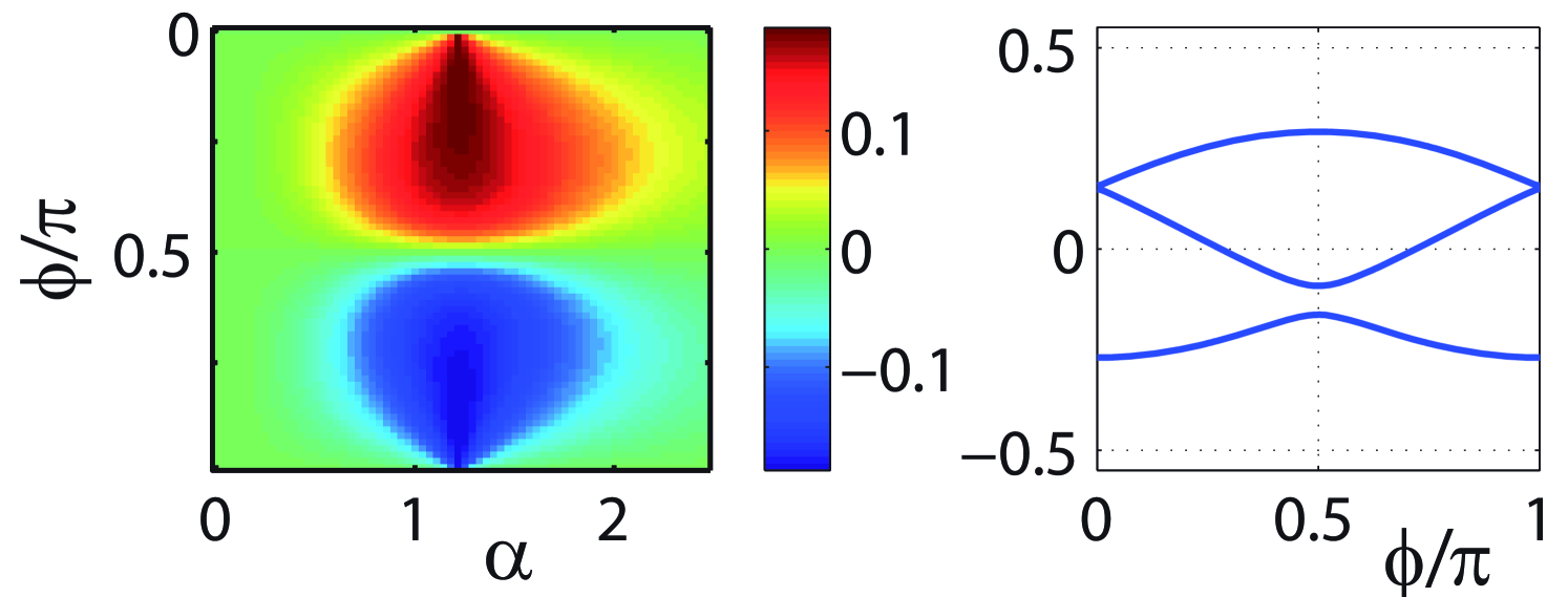
We show the current amplitude $\mathcal{C}$ in the left panel of figure 3 for different parameters $\alpha$ and $\phi$ . As explained above, it attains its maximum at $\alpha_{\rm opt}\simeq 1.2$ when both terms of the driving potential have the same weight, it is periodic in $\phi$ with $\pi$ periodicity and has vanishing values for $\phi=l\pi/2$ with $l$ integer. For $\phi_{\rm opt}\simeq\pm\pi/4$ one can see in the right panel of fig. 3 that the quasienergies become equidistant and thus there is only one relevant energy scale $\Delta\varepsilon_{f}=0.205V^{2}/\omega$ in the sum in Eq. (11) while the other sinusoidals oscillate with half this frequency. One can then average $\mathcal{I}_{m}$ over different periods to obtain $\mathcal{I}$ which achieves its maximum $\mathcal{I}(t_{\rm e}=n_{\rm e}T)\simeq M$ after $n_{\rm e}=1.81(V/\omega)^{-2}$ cycles as shown in fig. 1 b).

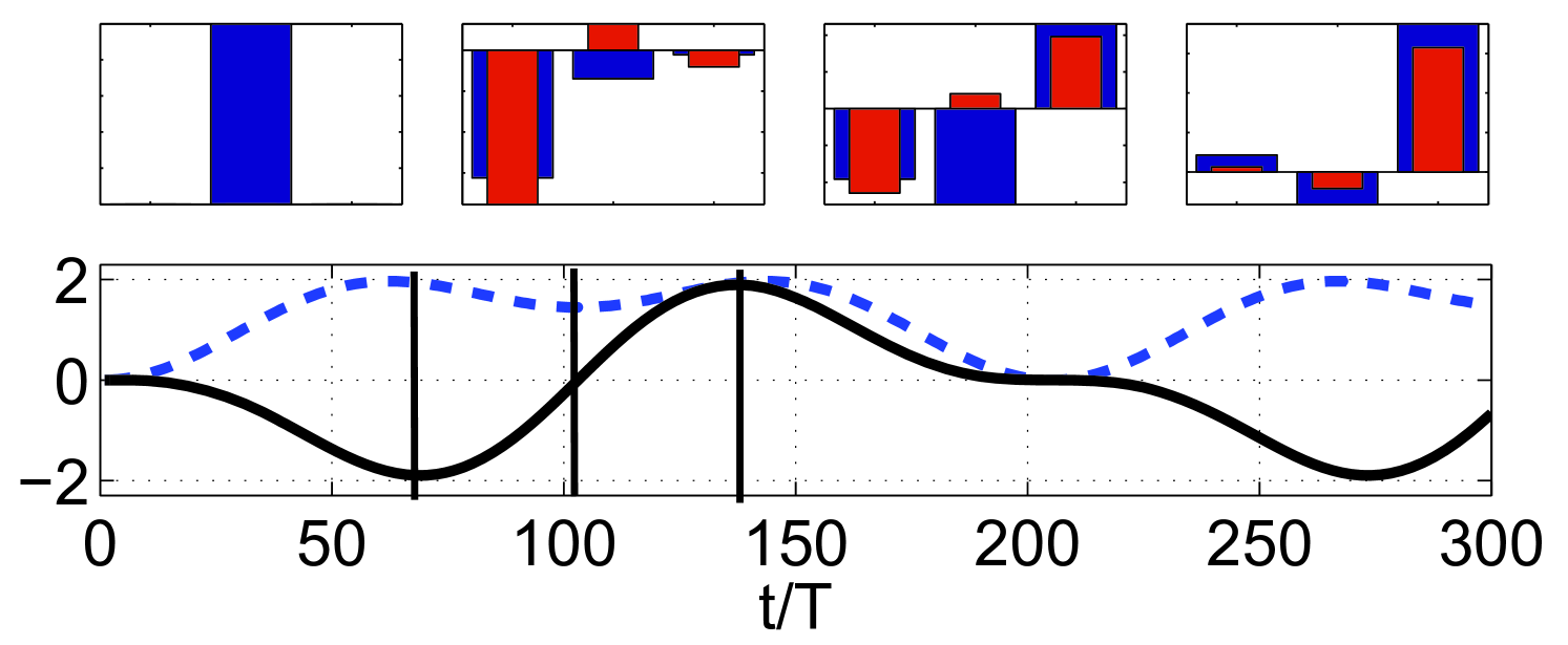
In the context of cold atoms it may be of interest not only the generation of a current from an initial zero momentum state, but also the control of the quantum state of the system. We plot in fig. 4 the particle state in the momentum basis and the average current per cycle and the average kinetic energy $\int_{0}^{T}dt\langle H_{0}\rangle/T$. We observe that the zero momentum state can be indeed converted into an almost pure momentum state $\left|\,\pm 2M\right\rangle$. One could then switch off the driving, thus breaking the time reversal symmetry $S_{t}$, and use this scheme to generate an asymptotic current. This is an example of the high controllability of our system.

Finally, let us analyze the feasibility of the model. We can summarise our findings in a simple recipe. $H_{0}$ sets the energy scale $J$ and the length $L$ of the system. We can obtain a final average current $\mathcal{I}$ of nearly $(L-1)/8$ in recoil units for a given time interval $[0,t_{\rm e}]$ if one tunes a driving potential in Eq. (5) with parameters $\omega$ from Eq. (6), $M_{\rm opt}$, $\alpha_{\rm opt}$, $\phi_{\rm opt}$ defined above and $V=\sqrt{11.37J(1-\cos(4\pi M_{\rm opt}/L))/t_{\rm e}}$ with the constraint that $V/J\leq 1$. We show in fig 3 that small changes in $\alpha$ and $\phi$ around optimal values only slightly affect the current. Smaller $M$ would reduce the maximum average current attained and require adjustment of the resonance condition in Eq.(6). Thus the only actual requirements of our model are that the system is tuned to resonance and that the driving field is weakly coupled. To show the robustness of the method we plot in figure 5 the average current when the system is not perfectly tuned to resonance and when the driving field is stronger. We find that couplings up to $V/\omega=0.5$ and errors of $1\%$ in the resonant frequency still give rise to high particle currents. Note that due to the resonance condition at low driving the effect is highly selective. If the initial state is a narrow wavepacket centered at $k=0$ only this component is mixed to $k=2M$, whereas other $k\leq M$ components remain uncoupled. The reduced average current will be just proportional to the weight of $k=0$ state, see fig. 5.

We have presented a model system where one can obtain currents with amplitudes orders of magnitude larger than those observed in recent experiments with coherent ratchet currents Salger_2009 . The oscillation period of the current can be controlled by the amplitude of the driving potential and in particular, by decreasing the driving strength one obtains currents which do not decay during the lifetime of the experiment. This effect is obtained with a potential which does not break the time-reversal symmetry and is due to crossed terms between the cyclic states of the system. The proposed scheme requires that the system is tuned to resonance and that the driving potential is weakly coupled such that only a few cyclic states are involved in the dynamics. We have checked the robustness of the method by tuning the system out of resonance and increasing the coupling strength. Furthermore, we have shown that it is possible to control the quantum state and the amount of kinetic energy in the system, using the proposed scheme to convert a zero momentum state into a state with high finite momentum, and viceversa.

We acknowledge support from the Spanish MICINN through projects FIS2007-61686, FIS2009-07277, FIS2010-18799 and the Ramón y Cajal programme.

References

- (1) P. Reimann, Phys. Rep. 361, 57 (2002).
- (2) P. Hänggi, F. Marchesoni, Rev. Mod. Phys. 81, 387 (2009).
- (3) F. Jülicher, A. Ajdari, J. Prost, Rev. Mod. Phys. 69, 1269 (1997).
- (4) H. Schanz, M.-F. Otto, R. Ketzmerick, T. Dittrich, Phys. Rev. Lett. 87, 070601 (2001); H. Schanz, T. Dittrich, R. Ketzmerick, Phys. Rev. E 71, 026228 (2005).
- (5) S. Flach, O. Yevtushenko, Y. Zolotaryuk, Phys. Rev. Lett. 84, 2358 (2000).
- (6) S. Denisov, L. Morales-Molina, S. Flach, P. Hänggi, Phys. Rev. A 75, 063424 (2007).
- (7) P. Reimann, M. Grifoni, P. Hänggi, Phys. Rev. Lett. 79, 10 (1997).
- (8) H. Linke et al., Science 286, 2314 (1999); J.B. Majer, J. Peguiron, M. Grifoni, M. Tusveld, J.E. Mooij, Phys. Rev. Lett. 90, 056802 (2003); M. V. Costache and S. O. Valenzuela, Science 330, 1645 (2010).
- (9) M. Schiavoni, L. Sánchez-Palencia, F. Renzoni, G. Grynberg, Phys. Rev. Lett. 90, 094101 (2003).
- (10) R. Gommers, S. Bergamini, F. Renzoni, Phys. Rev. Lett. 95, 073003 (2005); R. Gommers, S. Denisov, F. Renzoni, Phys. Rev. Lett. 96, 240604 (2006).
- (11) P.H. Jones, M. Goonasekera, D.R. Meacher, T. Jockheree, T. S. Monteiro, Phys. Rev. Lett. 98, 073002 (2007).
- (12) I.Dana and V. Roitberg, Phys. Rev. E 76, 015201(R) (2007); I. Dana, V. Ramareddy, I. Talukdar, and G. S. Summy, Phys. Rev. Lett. 100, 024103 (2008); I. Dana, Phys. Rev. E 81, 036210 (2010).
- (13) T. Salger, S. Kling, T. Hecking, C. Geckeler, L. Morales-Molina, M. Weitz, Science 326, 1241 (2009).
- (14) S. Denisov, L. Morales-Molina and S. Flach, E. Phys. Lett. 79, 10007 (2007).
- (15) D. Poletti, G. Benenti, G. Casati, P. Hänggi and B. Li, Phys. Rev. Lett 102,130604 (2009).
- (16) C. E. Creffield and F. Sols, Phys. Rev. Lett. 103, 200601 (2009).
- (17) G. Benenti, G. Casati, S. Denisov, S. Flach, P. Hänggi, B. Li, and D. Poletti , Phys. Rev. Lett. 104 228901 (2010).
- (18) C. E. Creffield and F. Sols, Phys. Rev. Lett. 104 228902 (2010) and supplementary material.
- (19) M. Moskalets and M. Büttiker, Phys. Rev. B 66, 205320 (2002).
- (20) E. Lundh and M. Wallin, Phys. Rev. Lett. 94, 110603 (2005).
- (21) J. Pelc, J. Gong, and P. Brumer, Phys. Rev. E 79, 066207 (2009).
- (22) J. H. Shirley, Phys. Rev. 138, B979 (1965).
- (23) I. Goychuk and P. Hänggi, J. Phys. Chem. B 105, 6642 (2001).
- (24) J. Ortigoso et al., J. Chem. Phys. 132, 074105 (2010).
- (25) H. Lignier, J.C. Garreau, P. Szriftgiser, D. Delande, Eur. Phys. Lett. 69, 327 (2005).
- (26) S. Franke- Arnold et al, Opt. Express 15, 8619 (2007); L. Amico, A. Osterloh and F. Cataliotti, Phys. Rev. Lett. 95, 063201 (2005); I. Ricardez-Vargas, K. Volke-Sepulveda J. Opt. Soc Am B 27, 948 (2010).
- (27) M. Heimsoth, C. E. Creffield, F. Sols, Phys. Rev. A 82, 023607(2010).
- (28) E. N. Economou, Green’s Functions in Quantum Physics Springer Series in Solid-State Sciences, 2009.