This paper was converted on www.awesomepapers.org from LaTeX by an anonymous user.
Want to know more? Visit the Converter page.

Tangential Navier-Stokes equations on evolving surfaces: Analysis and simulationsthanks: This work was partially supported by US National Science Foundation (NSF) through grants DMS-1953535 and DMS-2011444.

Maxim A. Olshanskii Department of Mathematics, University of Houston, Houston, Texas 77204 (molshan@math.uh.edu)    Arnold Reusken Institut für Geometrie und Praktische Mathematik, RWTH-Aachen University, D-52056 Aachen, Germany (reusken@igpm.rwth-aachen.de)    Alexander Zhiliakov Department of Mathematics, University of Houston, Houston, Texas 77204 (alex@math.uh.edu)
Abstract

The paper considers a system of equations that models a lateral flow of a Boussinesq–Scriven fluid on a passively evolving surface embedded in 3\mathbb{R}^{3}. For the resulting Navier-Stokes type system, posed on a smooth closed time-dependent surface, we introduce a weak formulation in terms of functional spaces on a space-time manifold defined by the surface evolution. The weak formulation is shown to be well-posed for any finite final time and without smallness conditions on data. We further extend an unfitted finite element method, known as TraceFEM, to compute solutions to the fluid system. Convergence of the method is demonstrated numerically. In another series of experiments we visualize lateral flows induced by smooth deformations of a material surface.

1 Introduction

There is extensive literature on analysis and numerical simulation of the incompressible Navier-Stokes equations, a fundamental model of fluid mechanics. While the overwhelming majority of papers in this field treats these equations in Euclidean domains, there also is literature on analysis of the incompressible Navier-Stokes equations on surfaces, or more general on Riemannian manifolds. Building on a fundamental observation made by Arnold [2] that relates equations of incompressible fluid to finding geodesics on the group of all volume preserving diffeomorphisms, local existence and uniqueness results for Navier-Stokes equations on compact oriented Riemannian manifolds were proved in the seminal paper [11]. This work has been followed by many other studies, cf. [44, 42] and the overview in [8]. Very recent activity in the field includes the work [33, 40], in which local-in-time-well-posedness in the framework of maximal regularity is established. All these papers restrict to stationary surfaces or manifolds.

In recent years there has been a growing interest in fluid equations on evolving surfaces [47, 20, 16, 24, 38], motivated in particular by applications to modeling of biological membranes, e.g. [39, 34, 4, 45]. In [6] one finds an overview and comparison of different modeling approaches for evolving viscous fluid layers that result in the surface Navier-Stokes equations. We are not aware of any literature presenting well-posedness analysis of this system on evolving surfaces. Furthermore, only very few papers address numerical treatment of such equations. In [36, 37] computational results are presented, based on a surface vorticity-stream function formulation of the Navier-Stokes equations. The surface motion is prescribed and the evolving SFEM of Dziuk-Elliott [9, 10] is applied to the partial differential equations for the scalar vorticity and stream function unknowns. The authors of [26] consider another discretization approach that is based on the techniques developed in [38]. These papers focus on modeling and illustration of certain interesting flow phenomena but not on the performance of the numerical methods. Several recent papers [17, 5, 14, 19] present error analysis of finite element discretization methods for vector valued PDEs on stationary surfaces. We are not aware of any paper with a systematic numerical study or an error analysis of a discretization method for vector valued PDEs on evolving surfaces. We conclude that in the field of incompressible Navier-Stokes equations on time-dependent surfaces basic problems related to well-posedness of the systems, development and analysis of numerical methods remain open. This paper addresses two of these problems: well-posedness and numerical method development.

It is shown in [6] that several different modeling approaches all yield the same tangential surface Navier-Stokes equations (TSNSE). These equations govern the evolution of tangential velocity and surface pressure if the normal velocity of the surface is prescribed. The main topic of the present paper is the analysis of a variational formulation of the TSNSE. In particular, a well-posedness result for this formulation is proved. To the best of our knowledge, this is the first well-posedness result for evolving surface Navier-Stokes equations. The paper also touches on the development of a new discretization method for the TSNSE. This method combines an implicit time stepping scheme with a TraceFEM [27, 30] for discretization in space. We explain this method, validate its optimal second order convergence for a test problem with a known solution and apply it to the simulation of a lateral flow induced by deformations of a sphere. Error analysis of this method is not addressed in this paper and left for future research.

The remainder of the paper is organized as follows. In section 2 we recall the surface Navier-Stokes equations known from the literature. In particular, the tangential surface Navier-Stokes equations are described. Appropriate function spaces for a variational formulation of the TSNSE are introduced in section 3. Relevant properties of these spaces are derived. The main results of this paper are given in section 4. We introduce and analyze two variational formulations of the TSNE: The first one is for the tangential velocity only, which is solenoidal by construction of the solution space. Then we introduce the pressure and study a mixed variational problem. For both formulations well-posedness results are derived. In section 5 we explain a discretization method. Finally, section 6 collects and discusses results of numerical experiments.

2 Surface Navier–Stokes equations

We first introduce necessary notations of surface quantities and tangential differential operators. For a closed smooth surface Γ\Gamma embedded in 3\mathbb{R}^{3}, the outward pointing normal vector is denoted by 𝐧\mathbf{n}, and the normal projector on the tangential space at 𝐱Γ\mathbf{x}\in\Gamma is 𝐏=𝐏(𝐱)=𝐈𝐧𝐧T\mathbf{P}=\mathbf{P}(\mathbf{x})=\mathbf{I}-\mathbf{n}\mathbf{n}^{T}. Let 𝐇=Γ𝐧3×3\mathbf{H}=\nabla_{\Gamma}\mathbf{n}\in\mathbb{R}^{3\times 3} be the Weingarten mapping (second fundamental form) and κ:=tr(𝐇)\kappa:={\rm tr}(\mathbf{H}) twice the mean curvature. For a scalar function p:Γp:\,\Gamma\to\mathbb{R} or a vector field 𝐮:Γ3\mathbf{u}:\,\Gamma\to\mathbb{R}^{3} their smooth extensions to a neighborhood 𝒪(Γ)\mathcal{O}(\Gamma) of Γ\Gamma are denoted by pep^{e} and 𝐮e\mathbf{u}^{e}, respectively. Surface gradients and covariant derivatives on Γ\Gamma can be defined through derivatives in 3\mathbb{R}^{3} as Γp=𝐏pe\nabla_{\Gamma}p=\mathbf{P}\nabla p^{e}, DΓ𝐮𝐮e𝐏D_{\Gamma}\mathbf{u}\coloneqq\nabla\mathbf{u}^{e}\mathbf{P}, and Γ𝐮𝐏𝐮e𝐏\nabla_{\Gamma}\mathbf{u}\coloneqq\mathbf{P}\nabla\mathbf{u}^{e}\mathbf{P}. These definitions are independent of a particular smooth extension of pp and 𝐮\mathbf{u} off Γ\Gamma. The surface rate-of-strain tensor [13] is given by Es(𝐮)12(Γ𝐮+Γ𝐮T)E_{s}(\mathbf{u})\coloneqq\frac{1}{2}(\nabla_{\Gamma}\mathbf{u}+\nabla_{\Gamma}\mathbf{u}^{T}), the surface divergence and curlΓ\operatorname{curl}_{\Gamma} operators for a vector field 𝐮:Γ3\mathbf{u}:\Gamma\to\mathbb{R}^{3} are divΓ𝐮tr(Γ𝐮){\mathop{\,\rm div}}_{\Gamma}\mathbf{u}\coloneqq{\rm tr}(\nabla_{\Gamma}\mathbf{u}) and curlΓ𝐮(Γ×𝐮)𝐧\operatorname{curl}_{\Gamma}\mathbf{u}\coloneqq(\nabla_{\Gamma}\times\mathbf{u})\cdot\mathbf{n}. For a tensor field 𝐀=[𝐚1,𝐚2,𝐚3]:Γ3×3\mathbf{A}=[\mathbf{a}_{1},\mathbf{a}_{2},\mathbf{a}_{3}]:\Gamma\to\mathbb{R}^{3\times 3} , divΓ𝐀{\mathop{\,\rm div}}_{\Gamma}\mathbf{A} is defined row-wise and DΓ𝐀D_{\Gamma}\mathbf{A} is a third-order tensor such that (DΓ𝐀)i,j,k=(DΓ𝐚j)i,k\big{(}D_{\Gamma}\mathbf{A}\big{)}_{i,j,k}=\big{(}D_{\Gamma}\mathbf{a}_{j}\big{)}_{i,k}.

We now let Γ(t)\Gamma(t) be a material surface embedded in 3\mathbb{R}^{3} as defined in [13, 25], with a density distribution ρ(t,𝐱)\rho(t,\mathbf{x}). By 𝐮(t,𝐱)\mathbf{u}(t,\mathbf{x}), 𝐱Γ(t)\mathbf{x}\in\Gamma(t), we denote a velocity field of the density flow on Γ\Gamma, i.e. 𝐮(t,𝐱)\mathbf{u}(t,\mathbf{x}) is the velocity of a material point 𝐱Γ(t)\mathbf{x}\in\Gamma(t). The derivative f.\accentset{\mbox{\large.}}{f} of a surface quantity ff along the corresponding trajectories of material points is called the material derivative. Assuming the surface evolution is such that the space-time manifold

𝒮=t[0,T]{t}×Γ(t)4\mathcal{S}=\bigcup\limits_{t\in[0,T]}\{t\}\times\Gamma(t)\subset\mathbb{R}^{4}

is smooth, the material derivative can be defined as

f.=fet+(𝐮)feon𝒮,\accentset{\mbox{\large.}}{f}=\frac{\partial f^{e}}{\partial t}+(\mathbf{u}\cdot\nabla)f^{e}\quad\text{on}~{}\mathcal{S}, (2.1)

where fef^{e} is a smooth extension of f:𝒮f:\,\mathcal{S}\to\mathbb{R} into a spatial neighborhood of 𝒮\mathcal{S}. Note that f.\accentset{\mbox{\large.}}{f} is a tangential derivative for 𝒮\mathcal{S}, and hence it depends only on the surface values of ff on 𝒮\mathcal{S}. For a vector field 𝐯\mathbf{v} on 𝒮\mathcal{S}, one defines 𝐯.\accentset{\mbox{\large.}}{\mathbf{v}} componentwise.

The conservation of mass and linear momentum for a thin material layer represented by Γ(t)\Gamma(t) together with the Boussinesq–Scriven constitutive relation for the surface stress tensor and an inextensibility condition leads to the surface Navier-Stokes equations:

{ρ𝐮.=Γπ+2μdivΓ(Es(𝐮))+𝐛+πκ𝐧divΓ𝐮=0ρ.=0onΓ(t),\left\{\begin{split}\rho\accentset{\mbox{\large.}}{\mathbf{u}}&=-\nabla_{\Gamma}\pi+2\mu{\mathop{\,\rm div}}_{\Gamma}(E_{s}(\mathbf{u}))+\mathbf{b}+\pi\kappa\mathbf{n}\\ {\mathop{\,\rm div}}_{\Gamma}\mathbf{u}&=0\\ \accentset{\mbox{\large.}}{\rho}&=0\end{split}\right.\qquad\text{on}~{}\Gamma(t), (2.2)

where π\pi is the surface fluid pressure and μ\mu stands for the viscosity coefficient. Equations (2.2) model the evolution of an inextensible viscous fluidic material surface with acting area force 𝐛\mathbf{b}, cf. [20, 16] for derivations of this model and [6] for a literature overview and alternative forms of this system. The pure geometrical evolution of Γ(t)\Gamma(t) is defined by its normal velocity VΓ=VΓ(t)V_{\Gamma}=V_{\Gamma}(t) that is given by the normal component of the material velocity,

VΓ=𝐮𝐧onΓ(t).V_{\Gamma}=\mathbf{u}\cdot\mathbf{n}\quad\text{on}~{}\Gamma(t). (2.3)

If 𝐛\mathbf{b} is given or defined through other unknowns, then (2.2)–(2.3) form a closed system of six equations for six unknowns 𝐮\mathbf{u}, π\pi, ρ\rho, and VΓV_{\Gamma}, subject to suitable initial conditions.

2.1 Tangential surface Navier-Stokes equations

We now introduce a major simplification by assuming that the geometric evolution of Γ\Gamma is known. We make this more precise below and derive equations governing the unknown lateral motions of the surface fluid. To this end, consider a smooth velocity field 𝐰=𝐰(t,𝐱)\mathbf{w}=\mathbf{w}(t,\mathbf{x}) in [0,T]×3[0,T]\times\mathbb{R}^{3} that passively advects the embedded surface Γ(t)\Gamma(t) given by

Γ(t)={𝐲3|𝐲=𝐱(t,𝐳),𝐳Γ0},\Gamma(t)=\{\mathbf{y}\in\mathbb{R}^{3}~{}|~{}\mathbf{y}=\mathbf{x}(t,\mathbf{z}),~{}\mathbf{z}\in\Gamma_{0}\}, (2.4)

where the trajectories 𝐱(t,𝐳)\mathbf{x}(t,\mathbf{z}) are the unique solutions of the Cauchy problem

{𝐱(0,𝐳)=𝐳ddt𝐱(t,𝐳)=𝐰(t,𝐱(t,𝐳)),\displaystyle\begin{cases}\mathbf{x}(0,\mathbf{z})=\mathbf{z}\\ \frac{d}{dt}\mathbf{x}(t,\mathbf{z})=\mathbf{w}(t,\mathbf{x}(t,\mathbf{z})),\end{cases} (2.5)

for all 𝐳\mathbf{z} on an initial smooth connected surface Γ0=Γ(0)\Gamma_{0}=\Gamma(0) embedded in 3\mathbb{R}^{3}. We now assume that the normal material motion of Γ\Gamma is completely determined by the ambient flow 𝐰\mathbf{w} and the lateral material motion is free, i.e., for the given 𝐰\mathbf{w} the relation

𝐮𝐧=𝐰𝐧onΓ(t)\mathbf{u}\cdot\mathbf{n}=\mathbf{w}\cdot\mathbf{n}\quad\text{on}~{}\Gamma(t) (2.6)

holds for the normal component111For velocity fields 𝐯3\mathbf{v}\in\mathbb{R}^{3} defined on Γ(t)\Gamma(t) we use a splitting into tangential and normal components 𝐯=𝐯T+𝐯N=𝐯T+vN𝐧\mathbf{v}=\mathbf{v}_{T}+\mathbf{v}_{N}=\mathbf{v}_{T}+v_{N}\mathbf{n}, with vN=𝐯𝐧v_{N}=\mathbf{v}\cdot\mathbf{n}. uN=𝐮𝐧u_{N}=\mathbf{u}\cdot\mathbf{n}, while the tangential component 𝐮T\mathbf{u}_{T} of the surface fluid flow is unknown and depends on 𝐰\mathbf{w} only implicitly through the variation of Γ(t)\Gamma(t) and conservation laws represented by equations (2.2). The resulting system can be seen as an idealized model for the motion of a fluid layer embedded in bulk fluid, where one neglects friction forces between the surface and bulk fluids as well as any effect of the layer on the bulk flow. In such a physical setting, (2.6) means non-penetration of the bulk fluid through the material layer.

Material trajectories of points on the surface are defined by the flow field 𝐮\mathbf{u}, rather than 𝐰\mathbf{w}. We are also interested in a derivative determined by the variation of a quantity along the so-called normal trajectories defined below.

Definition 1.

Let Φtn:Γ0Γ(t)\Phi_{t}^{n}:\,\Gamma_{0}\to\Gamma(t), be the flow map of the pure geometric (normal) evolution of the surface, i.e., for 𝐳Γ0\mathbf{z}\in\Gamma_{0}, the normal trajectory 𝐱n(t,𝐳)=Φtn(𝐳)\mathbf{x}^{n}(t,\mathbf{z})=\Phi_{t}^{n}(\mathbf{z}) solves

{𝐱n(0,𝐳)=𝐳,ddt𝐱n(t,𝐳)=𝐰N(t,𝐱n(𝐳,t)).\displaystyle\begin{cases}\mathbf{x}^{n}(0,\mathbf{z})=\mathbf{z},\\ \frac{d}{dt}\mathbf{x}^{n}(t,\mathbf{z})=\mathbf{w}_{N}(t,\mathbf{x}^{n}(\mathbf{z},t)).\end{cases} (2.7)

Eq. (2.7) defines a bijection between Γ0\Gamma_{0} and Γ(t)\Gamma(t) for every t[0,T]t\in[0,T] with inverse mapping Φtn\Phi_{-t}^{n}. The Lagrangian derivative for the flow map Φtn\Phi_{t}^{n} is denoted by \partial^{\circ}:

𝐯(t,𝐱)=ddt𝐯(t,Φtn(𝐳)),𝐱=Φtn(𝐳).\partial^{\circ}\mathbf{v}(t,\mathbf{x})=\frac{d}{dt}\mathbf{v}(t,\Phi_{t}^{n}(\mathbf{z})),\quad\mathbf{x}=\Phi_{t}^{n}(\mathbf{z}). (2.8)

We call 𝐯\partial^{\circ}\mathbf{v} the normal time derivative of 𝐯\mathbf{v}.

It is clear from (2.8) that this normal time derivative is an intrinsic surface quantity. Similar to the material derivative in (2.1), it can be expressed in terms of bulk derivatives if one assumes a smooth extension of 𝐯\mathbf{v} from 𝒮\mathcal{S} to its neighborhood:

𝐯(t,𝐱)=ddt𝐯(t,𝐱n(t,𝐳))=(𝐯et+(𝐰N)𝐯e)(t,𝐱)\partial^{\circ}\mathbf{v}(t,\mathbf{x})=\frac{d}{dt}\mathbf{v}(t,\mathbf{x}^{n}(t,\mathbf{z}))=\Big{(}\frac{\partial\mathbf{v}^{e}}{\partial t}+(\mathbf{w}_{N}\cdot\nabla)\mathbf{v}^{e}\Big{)}(t,\mathbf{x}) (2.9)

for (t,𝐱)𝒮(t,\mathbf{x})\in\mathcal{S}. Comparing the material and normal time derivatives of a flow field 𝐯\mathbf{v} on the surface we find the equality

𝐏𝐯.=𝐏𝐯+(Γ𝐯)𝐮T.\mathbf{P}\accentset{\mbox{\large.}}{\mathbf{v}}=\mathbf{P}\partial^{\circ}\mathbf{v}+(\nabla_{\Gamma}\mathbf{v})\mathbf{u}_{T}.

With the splitting 𝐯=𝐯T+𝐯N\mathbf{v}=\mathbf{v}_{T}+\mathbf{v}_{N} we get

𝐏𝐯.=𝐏𝐯T+𝐏𝐯N+(Γ𝐯T)𝐮T+(Γ𝐯N)𝐮T.\mathbf{P}\accentset{\mbox{\large.}}{\mathbf{v}}=\mathbf{P}\partial^{\circ}\mathbf{v}_{T}+\mathbf{P}\partial^{\circ}\mathbf{v}_{N}+(\nabla_{\Gamma}\mathbf{v}_{T})\mathbf{u}_{T}+(\nabla_{\Gamma}\mathbf{v}_{N})\mathbf{u}_{T}. (2.10)

Noting that 𝐏𝐧=0\mathbf{P}\mathbf{n}=0 and 𝐏𝐧=ΓwN\mathbf{P}\partial^{\circ}\mathbf{n}=-\nabla_{\Gamma}w_{N} (cf. (2.16) in [16]), we rewrite 𝐏𝐯N\mathbf{P}\partial^{\circ}\mathbf{v}_{N} as

𝐏𝐯N=vN𝐏𝐧+vN𝐏𝐧=vN𝐏𝐧=vNΓwN.\mathbf{P}\partial^{\circ}\mathbf{v}_{N}=\partial^{\circ}v_{N}\mathbf{P}\mathbf{n}+v_{N}\mathbf{P}\partial^{\circ}\mathbf{n}=v_{N}\mathbf{P}\partial^{\circ}\mathbf{n}=-v_{N}\nabla_{\Gamma}w_{N}.

We also have the relation (Γ𝐯N)𝐮T=vN𝐇𝐮T(\nabla_{\Gamma}\mathbf{v}_{N})\mathbf{u}_{T}=v_{N}\mathbf{H}\mathbf{u}_{T}. Using these results and letting 𝐯=𝐮\mathbf{v}=\mathbf{u} in (2.10) one obtains

𝐏𝐮.=𝐏𝐮T+(Γ𝐮T)𝐮T+wN𝐇𝐮T12ΓwN2,\mathbf{P}\accentset{\mbox{\large.}}{\mathbf{u}}=\mathbf{P}\partial^{\circ}\mathbf{u}_{T}+(\nabla_{\Gamma}\mathbf{u}_{T})\mathbf{u}_{T}+w_{N}\mathbf{H}\mathbf{u}_{T}-\tfrac{1}{2}\nabla_{\Gamma}w_{N}^{2}, (2.11)

where we also used uN=wNu_{N}=w_{N}. To derive an equation for the unknown tangential velocity 𝐮T\mathbf{u}_{T}, we apply the projection 𝐏\mathbf{P} to the first equation in (2.2). For 𝐏𝐮.\mathbf{P}\accentset{\mbox{\large.}}{\mathbf{u}} we have the result (2.11). Note that the term 12ΓwN2\tfrac{1}{2}\nabla_{\Gamma}w_{N}^{2} is known and can be treated as a source term. For a stationary surface (wN=0w_{N}=0) the normal time derivative is just the usual time derivative, 𝐏𝐮T=𝐮Tt\mathbf{P}\partial^{\circ}\mathbf{u}_{T}=\frac{\partial\mathbf{u}_{T}}{\partial t}. The term (Γ𝐮T)𝐮T(\nabla_{\Gamma}\mathbf{u}_{T})\mathbf{u}_{T} is the analog of the quadratic term in Navier-Stokes equations. Using divΓ𝐮N=uNκ{\mathop{\,\rm div}}_{\Gamma}\mathbf{u}_{N}=u_{N}\kappa and uN=wNu_{N}=w_{N}, the second equation in (2.2) yields divΓ𝐮T=wNκ{\mathop{\,\rm div}}_{\Gamma}\mathbf{u}_{T}=-w_{N}\kappa. We are not interested in variable density case and let ρ=1\rho=1. Summarizing, from the surface Navier-Stokes equations (2.2) we get the following reduced system for 𝐮T\mathbf{u}_{T} and π\pi which we call the tangential surface Navier-Stokes equations (TSNSE):

{𝐏𝐮T+(Γ𝐮T)𝐮T+wN𝐇𝐮T2μ𝐏divΓEs(𝐮T)+Γπ=𝐟divΓ𝐮T=g,\left\{\begin{aligned} \mathbf{P}\partial^{\circ}\mathbf{u}_{T}+(\nabla_{\Gamma}\mathbf{u}_{T})\mathbf{u}_{T}+w_{N}\mathbf{H}\mathbf{u}_{T}-2\mu\mathbf{P}{\mathop{\,\rm div}}_{\Gamma}E_{s}(\mathbf{u}_{T})+\nabla_{\Gamma}\pi&=\mathbf{f}\\ {\mathop{\,\rm div}}_{\Gamma}\mathbf{u}_{T}&=g,\\ \end{aligned}\right. (2.12)

with right-hand sides known in terms of geometric quantities, wNw_{N} and the tangential component of the external area force 𝐛\mathbf{b}:

g=wNκ,𝐟=𝐛T+2μ𝐏divΓ(wN𝐇)+12ΓwN2.g=-w_{N}\kappa,\qquad\mathbf{f}=\mathbf{b}_{T}+2\mu\mathbf{P}{\mathop{\,\rm div}}_{\Gamma}(w_{N}\mathbf{H})+\tfrac{1}{2}\nabla_{\Gamma}w_{N}^{2}. (2.13)

In the remainder of this paper we study this TSNSE. Note that these equations have a structure similar to the standard incompressible Navier-Stokes equations in Euclidean domains. Important differences are that TSNSE is formulated on a space-time manifold that does not have an evident tensor product structure and, related to this, a normal time derivative 𝐏\mathbf{P}\partial^{\circ} instead of the standard time derivative is used and an additional term wN𝐇𝐮Tw_{N}\mathbf{H}\mathbf{u}_{T} occurs. After some preliminary results in the next section, we introduce a well-posed weak formulation of the TSNSE in section 4.

Remark 2.1.

If one does not assume a given normal velocity uN=wNu_{N}=w_{N}, an equation for uNu_{N} can be derived from (2.2), cf. [16]. The surface Navier-Stokes equations (2.2) are then rewritten as a coupled system for 𝐮T\mathbf{u}_{T}, π\pi and uNu_{N}, that consists of TSNSE (2.12) and the coupled equation

u.N=2μ(tr(𝐇Γ𝐮T)+uNtr(𝐇2))+𝐮T𝐇𝐮T𝐮TΓuN+πκ+bN.\accentset{\mbox{\large.}}{u}_{N}=-2\mu\big{(}{\rm tr}(\mathbf{H}\nabla_{\Gamma}\mathbf{u}_{T})+u_{N}{\rm tr}(\mathbf{H}^{2})\big{)}+\mathbf{u}_{T}\cdot\mathbf{H}\mathbf{u}_{T}-\mathbf{u}_{T}\cdot\nabla_{\Gamma}u_{N}+\pi\kappa+b_{N}. (2.14)

A challenging problem, not addressed in this paper, is the well-posedness of the surface Navier-Stokes equations (2.2), i.e., of the coupled system (2.12)–(2.14). For studying this problem, results on well-posedness of only the TSNSE (2.12) may be useful.

3 Preliminaries

In this section we introduce several function spaces and derive relevant properties of these spaces. We will use these spaces to formulate a well-posed weak formulation of the TSNSE (2.12). At this point, we make our assumptions on Γ0\Gamma_{0} and its evolution more precise. We introduce the following smoothness assumptions:

Γ0C3and𝐰C3([0,T]×3,3),sup[0,T]×3|𝐰|<+.\Gamma_{0}\in C^{3}\quad\text{and}\quad\mathbf{w}\in C^{3}([0,T]\times\mathbb{R}^{3},\mathbb{R}^{3}),~{}\sup_{[0,T]\times\mathbb{R}^{3}}|\mathbf{w}|<+\infty. (3.1)

Then the ODE system (2.5) has a unique solution for any 𝐳Γ03\mathbf{z}\in\Gamma_{0}\subset\mathbb{R}^{3}, which defines a one-to-one mapping Γ0Γ(t)\Gamma_{0}\to\Gamma(t) for all t[0,T]t\in[0,T] (Theorems II.1.1, V.3.1 and remark to Theorem V.2.1 in [15]). Moreover, this mapping is C3(𝒮0,4)C^{3}(\mathcal{S}_{0},\mathbb{R}^{4}) (Corollary V.4.1 [15]) with

𝒮0:=[0,T]×Γ0.\mathcal{S}_{0}:=[0,T]\times\Gamma_{0}.

Therefore, 𝒮\mathcal{S} is a C3C^{3} manifold as the image of 𝒮0C3\mathcal{S}_{0}\in C^{3} under a smooth mapping.

We need a globally C2C^{2}-smooth extension of the spatial normal 𝐧(t,x)\mathbf{n}(t,x), (t,x)𝒮(t,x)\in\mathcal{S} that can be constructed as follows. Let ϕ0\phi_{0} be the signed distance function to Γ0\Gamma_{0}. On a tubular neighborhood UδU_{\delta} of Γ0\Gamma_{0}, with diameter δ>0\delta>0 sufficiently small, we have ϕ0C3(Uδ)\phi_{0}\in C^{3}(U_{\delta}), cf. [10, Lemma 2.8]. We extend this function to be from C3(3)C^{3}(\mathbb{R}^{3}) and zero outside U2δU_{2\delta}. Thus we have ϕ0C3(3)\phi_{0}\in C^{3}(\mathbb{R}^{3}) and ϕ0\phi_{0} is a signed distance function in a neighborhood of Γ0\Gamma_{0}. Let Φt\Phi_{t} be the flow map for the velocity field 𝐰\mathbf{w}. The mapping (t,𝐱)Φt(𝐱)(t,\mathbf{x})\to\Phi_{t}(\mathbf{x}) is C3([0,T]×3,3)C^{3}([0,T]\times\mathbb{R}^{3},\mathbb{R}^{3}) and xΦt(𝐱)\nabla_{x}\Phi_{t}(\mathbf{x}) is regular [15]. Define the level set function ϕ(t,x):=ϕ0(Φt(𝐱))\phi(t,x):=\phi_{0}\big{(}\Phi_{-t}(\mathbf{x})\big{)} and the neighborhood 𝒮ex:=t[0,T]{t}×Φt(Uδ)\mathcal{S}^{\rm ex}:=\cup_{t\in[0,T]}\{t\}\times\Phi_{t}(U_{\delta}) of 𝒮\mathcal{S}. Then we have ϕC3([0,T]×3,)\phi\in C^{3}([0,T]\times\mathbb{R}^{3},\mathbb{R}) and for (t,𝐱)𝒮ex(t,\mathbf{x})\in\mathcal{S}^{\rm ex} it holds |ϕ(t,x)|c>0|\nabla\phi(t,x)|\geq c>0, and ϕ(t,x)=0\phi(t,x)=0 iff (t,x)𝒮(t,x)\in\mathcal{S}. Set 𝐧^(t,𝐱):=ϕ(t,x)/|ϕ(t,x)|\hat{\mathbf{n}}(t,\mathbf{x}):=\nabla\phi(t,x)/|\nabla\phi(t,x)| for (t,𝐱)𝒮ex(t,\mathbf{x})\in\mathcal{S}^{\rm ex}. Clearly 𝐧^=𝐧\hat{\mathbf{n}}=\mathbf{n} on 𝒮\mathcal{S} and 𝐧^C2(𝒮ex,3)\hat{\mathbf{n}}\in C^{2}(\mathcal{S}^{\rm ex},\mathbb{R}^{3}), and by a standard procedure we can extend it to 𝐧^C2([0,T]×3,3)\hat{\mathbf{n}}\in C^{2}([0,T]\times\mathbb{R}^{3},\mathbb{R}^{3}). To simplify the notation, this extension is denoted by 𝐧\mathbf{n}. For such an extended vector field 𝐧\mathbf{n} we have that 𝐰N=(𝐰𝐧)𝐧C2([0,T]×3,3)\mathbf{w}_{N}=(\mathbf{w}\cdot\mathbf{n})\mathbf{n}\in C^{2}([0,T]\times\mathbb{R}^{3},\mathbb{R}^{3}) holds. Arguing in the same way as above, we conclude that for the normal flow mapping from definition 1 we have

Φ()nC2(𝒮0,𝒮).\Phi_{(\cdot)}^{n}\in C^{2}(\mathcal{S}_{0},\mathcal{S}). (3.2)

Note that 𝒮0=𝒮0¯\mathcal{S}_{0}=\overline{\mathcal{S}_{0}} and 𝒮=𝒮¯\mathcal{S}=\overline{\mathcal{S}}, i.e., 𝒮0\mathcal{S}_{0} and 𝒮\mathcal{S} are closed manifolds.
We need function spaces suitable for a weak formulation of the TSNSE. For this we make use of a general framework of evolving spaces presented in [1]. In section 3.2 we introduce specific evolving Hilbert spaces, based on a Piola pushforward mapping. Based on results from [1] several properties of these spaces are derived. In section 3.4 an evolving space of functions for which suitable weak “material” derivatives exist is introduced. Here we deviate from [1] in the sense that this “material” derivative is not based on the pushforward map but on the normal time derivative defined above.

3.1 Surface Piola transform

To define evolving Hilbert spaces based on standard Bochner spaces, we need a suitable pushforward map. In the context of this paper it is natural to use a surface Piola transform as pushforward map, since this transform conserves the solenoidal property of a tangential vector field.

To define a surface variant of the Piola transform based on the normal flow map Φtn:Γ0Γ(t)\Phi_{t}^{n}:\,\Gamma_{0}\to\Gamma(t), we need some further notation. Below we always take 𝐳Γ0\mathbf{z}\in\Gamma_{0} and 𝐱:=Φtn(𝐳)Γ(t)\mathbf{x}:=\Phi^{n}_{t}(\mathbf{z})\in\Gamma(t). Since for each t[0,T]t\in[0,T] the map Φtn:Γ0Γ(t)\Phi_{t}^{n}:\,\Gamma_{0}\to\Gamma(t) is a C2C^{2}-diffeomorphism, the differential DΦtn(𝐳):(TΓ0)𝐳TΓ(t)𝐱D\Phi_{t}^{n}(\mathbf{z}):\,(T\Gamma_{0})_{\mathbf{z}}\to T\Gamma(t)_{\mathbf{x}}, is invertible. Define J=J(t,𝐳):=detDΦtn(𝐳)J=J(t,\mathbf{z}):=\det D\Phi_{t}^{n}(\mathbf{z}), J1=J1(t,𝐱)=detDΦtn(𝐱)=J(t,𝐳)1J^{-1}=J^{-1}(t,\mathbf{x})=\det D\Phi_{-t}^{n}(\mathbf{x})=J(t,\mathbf{z})^{-1}. Denote by 𝐃=𝐃(t,𝐳)\mathbf{D}=\mathbf{D}(t,\mathbf{z}) and 𝐃1=𝐃1(t,𝐱)\mathbf{D}^{-1}=\mathbf{D}^{-1}(t,\mathbf{x}) the matrices of linear mappings given by DΦtn(𝐳)𝐏(𝐳):33D\Phi_{t}^{n}(\mathbf{z})\mathbf{P}(\mathbf{z}):\mathbb{R}^{3}\to\mathbb{R}^{3} and DΦtn(𝐱)𝐏(𝐱)=[DΦtn(𝐳)]1𝐏(𝐱):33D\Phi_{-t}^{n}(\mathbf{x})\mathbf{P}(\mathbf{x})=[D\Phi_{t}^{n}(\mathbf{z})]^{-1}\mathbf{P}(\mathbf{x}):\mathbb{R}^{3}\to\mathbb{R}^{3}, respectively. Note that 𝐃1𝐃=𝐏(𝐳)\mathbf{D}^{-1}\mathbf{D}=\mathbf{P}(\mathbf{z}) and 𝐃𝐃1=𝐏(𝐱)\mathbf{D}\mathbf{D}^{-1}=\mathbf{P}(\mathbf{x}) hold. For these mappings the following useful identities hold:

DΓ(𝐯Φtn)=(DΓ0𝐯)𝐃1for𝐯C1(Γ0)3,(DΓ𝐯)𝐃=DΓ0(𝐯Φtn)for𝐯C1(Γ(t))3.\begin{split}D_{\Gamma}\,(\mathbf{v}\circ\Phi_{-t}^{n})=\left(D_{\Gamma_{0}}\mathbf{v}\right)\mathbf{D}^{-1}\quad\text{for}~{}\mathbf{v}\in C^{1}(\Gamma_{0})^{3},\\ \left(D_{\Gamma}\,\mathbf{v}\right)\mathbf{D}=D_{\Gamma_{0}}(\mathbf{v}\circ\Phi_{t}^{n})\quad\text{for}~{}\mathbf{v}\in C^{1}\big{(}\Gamma(t)\big{)}^{3}.\end{split} (3.3)

We need the Piola transform for arbitrary, not necessarily tangential vectors. For this it is convenient to define an invertible operator 𝐀(t,𝐳):33{\mathbf{A}}(t,\mathbf{z}):\mathbb{R}^{3}\to\mathbb{R}^{3} such that 𝐀|TΓ0=J1DΦtn:TΓ0TΓ(t)\mathbf{A}|_{T\Gamma_{0}}=J^{-1}D\Phi_{t}^{n}:\,T\Gamma_{0}\to T\Gamma(t) and 𝐀:TΓ0TΓ(t)\mathbf{A}:T\Gamma_{0}^{\perp}\to T\Gamma(t)^{\perp}. We use the operator

𝐀(t,𝐳)𝐯:=J1(t,𝐱)𝐃(t,𝐳)𝐯+𝐧Γ(t)(𝐱)𝐧Γ0(𝐳)𝐯,𝐯3.{\mathbf{A}}(t,\mathbf{z})\mathbf{v}:=J^{-1}(t,\mathbf{x})\mathbf{D}(t,\mathbf{z})\mathbf{v}+\mathbf{n}_{\Gamma(t)}(\mathbf{x})\mathbf{n}_{\Gamma_{0}}(\mathbf{z})\cdot\mathbf{v}\,,\quad\mathbf{v}\in\mathbb{R}^{3}. (3.4)

For 𝐀1(t,𝐱):=J(t,𝐳)𝐃1(t,𝐱)+𝐧Γ0(𝐳)𝐧Γ(t)(𝐱)T{\mathbf{A}}^{-1}(t,\mathbf{x}):=J(t,\mathbf{z})\mathbf{D}^{-1}(t,\mathbf{x})+\mathbf{n}_{\Gamma_{0}}(\mathbf{z})\mathbf{n}_{\Gamma(t)}(\mathbf{x})^{T} it holds 𝐀1(t,𝐱)𝐀(t,𝐳)=I3{\mathbf{A}}^{-1}(t,\mathbf{x}){\mathbf{A}}(t,\mathbf{z})=I_{\mathbb{R}^{3}}. The matrices of 𝐀\mathbf{A} and 𝐀1\mathbf{A}^{-1} in the standard basis are also denoted by 𝐀\mathbf{A} and 𝐀1\mathbf{A}^{-1}, respectively. Note that det𝐀=1\det\mathbf{A}=1 holds. We define the surface Piola transform Pt:33P_{t}:\mathbb{R}^{3}\to\mathbb{R}^{3} by

(Pt𝐯)(𝐱):=𝐀(t,𝐳)𝐯(𝐳),𝐳Γ0.(P_{t}\mathbf{v})(\mathbf{x}):=\mathbf{A}(t,\mathbf{z})\,\mathbf{v}(\mathbf{z}),\quad\mathbf{z}\in\Gamma_{0}. (3.5)

This operator maps tangential vectors on Γ0\Gamma_{0} to tangential vectors on Γ(t)\Gamma(t) and for tangential vectors 𝐯\mathbf{v} it satisfies divΓPt𝐯=0{\mathop{\,\rm div}}_{\Gamma}P_{t}\mathbf{v}=0 a.e. on Γ(t)\Gamma(t) iff divΓ𝐯=0{\mathop{\,\rm div}}_{\Gamma}\mathbf{v}=0 a.e. on Γ0\Gamma_{0}, cf. [41].

We need some regularity properties of 𝐃\mathbf{D}, 𝐀\mathbf{A} and 𝐃1\mathbf{D}^{-1}, 𝐀1\mathbf{A}^{-1}, which are collected in the following lemma. For a function gC1(𝒮0)g\in C^{1}({\mathcal{S}}_{0}) the maximum norm is gC1(𝒮0):=max(t,𝐳)𝒮0(|g(t,𝐳)|+|S0g(t,𝐳)|)\|g\|_{C^{1}(\mathcal{S}_{0})}:=\max_{(t,\mathbf{z})\in\mathcal{S}_{0}}\big{(}|g(t,\mathbf{z})|+|\nabla_{S_{0}}g(t,\mathbf{z})|\big{)} and similarly for vector and matrix valued functions as well as for such functions on 𝒮\mathcal{S}.

Lemma 2.

It holds that 𝐃,𝐀C1(𝒮0)3×3\mathbf{D},\mathbf{A}\in C^{1}({\mathcal{S}}_{0})^{3\times 3}, 𝐃1,𝐀1C1(𝒮)3×3\mathbf{D}^{-1},\mathbf{A}^{-1}\in C^{1}({\mathcal{S}})^{3\times 3} and, in particular,

JC1(𝒮0)+𝐃C1(𝒮0)+𝐀C1(𝒮0)+J1C1(𝒮)+𝐃1C1(𝒮)+𝐀1C1(𝒮)C.\|J\|_{C^{1}({\mathcal{S}}_{0})}+\|\mathbf{D}\|_{C^{1}({\mathcal{S}}_{0})}+\|\mathbf{A}\|_{C^{1}({\mathcal{S}}_{0})}+\|J^{-1}\|_{C^{1}({\mathcal{S}})}+\|\mathbf{D}^{-1}\|_{C^{1}({\mathcal{S}})}+\|\mathbf{A}^{-1}\|_{C^{1}({\mathcal{S}})}\leq C. (3.6)
Proof.

From (3.2) we know that Φ:(t,𝐳)(t,Φtn(𝐳))\Phi:(t,\mathbf{z})\to(t,\Phi_{t}^{n}(\mathbf{z})) is in C2(𝒮0,𝒮)C^{2}({\mathcal{S}}_{0},{\mathcal{S}}) and hence DΦC1(T𝒮0,T𝒮)D\Phi\in C^{1}(T{\mathcal{S}}_{0},T{\mathcal{S}}). Moreover, 𝐏𝒮0\mathbf{P}_{\mathcal{S}_{0}} is C1C^{1}-smooth, so DΦ𝐏𝒮0D\Phi\mathbf{P}_{\mathcal{S}_{0}} is a C1C^{1} smooth mapping with matrix representation

[1𝐰NT0𝐃]C1(𝒮0)4×4.\left[\begin{matrix}1&\mathbf{w}_{N}^{T}\\ 0&\mathbf{D}\end{matrix}\right]\in C^{1}({\mathcal{S}}_{0})^{4\times 4}. (3.7)

Hence, 𝐃C1(𝒮0)3×3\mathbf{D}\in C^{1}({\mathcal{S}}_{0})^{3\times 3} and JC1(𝒮0)J\in C^{1}({\mathcal{S}}_{0}) hold. Combining this with 𝐧Γ0,𝐧Γ()Φ()nC1(𝒮0)\mathbf{n}_{\Gamma_{0}},\mathbf{n}_{\Gamma(\cdot)}\circ\Phi_{(\cdot)}^{n}\in C^{1}({\mathcal{S}}_{0}), (3.4) and the property that 𝒮0\mathcal{S}_{0} is closed, implies the bound in (3.6) for 𝐃\mathbf{D}, JJ and 𝐀\mathbf{A}. The mapping Φ:𝒮0𝒮\Phi:\,\mathcal{S}_{0}\to\mathcal{S} is one-to-one. By the inverse mapping theorem the inverse Φ1\Phi^{-1} is C2(𝒮,𝒮0)C^{2}(\mathcal{S},{\mathcal{S}}_{0}) and for its differential we have DΦ1C1(T𝒮,T𝒮0)D\Phi^{-1}\in C^{1}(T{\mathcal{S}},T{\mathcal{S}}_{0}). The matrix of the C1C^{1} smooth mapping DΦ1𝐏𝒮D\Phi^{-1}\mathbf{P}_{\mathcal{S}} is

[1𝐰NT𝐃10𝐃1]C1(𝒮)4×4.\left[\begin{matrix}1&-\mathbf{w}_{N}^{T}\mathbf{D}^{-1}\\ 0&\mathbf{D}^{-1}\end{matrix}\right]\in C^{1}({\mathcal{S}})^{4\times 4}.

This and 𝐀1=J𝐃1+𝐧Γ0𝐧Γ()T(Φ()n){\mathbf{A}}^{-1}=J\mathbf{D}^{-1}+\mathbf{n}_{\Gamma_{0}}\mathbf{n}_{\Gamma(\cdot)}^{T}(\Phi_{(\cdot)}^{n}) imply the desired bound for 𝐃1\mathbf{D}^{-1}, J1J^{-1} and 𝐀1\mathbf{A}^{-1}. ∎

3.2 Evolving Hilbert spaces

For constructing suitable evolving Hilbert spaces, we first define tangential velocity spaces on Γ(t)\Gamma(t). The notation (,)0,t(\cdot,\cdot)_{0,t} and 0,t\|\cdot\|_{0,t} is used for the canonical inner product and norm in L2(Γ(t))L^{2}(\Gamma(t)). We need the Sobolev spaces of order one

H1(t):={𝐯H1(Γ(t))3|𝐯𝐧=0onΓ(t)},H^{1}(t):=\{\mathbf{v}\in H^{1}(\Gamma(t))^{3}~{}|~{}\mathbf{v}\cdot\mathbf{n}=0~{}~{}\text{on}~{}~{}\Gamma(t)\},

with the inner product (,)1,t:=(,)0,t+(DΓ,DΓ)0,t(\cdot,\cdot)_{1,t}:=(\cdot,\cdot)_{0,t}+(D_{\Gamma}\cdot,D_{\Gamma}\cdot)_{0,t}, and its closed subspace of divergence free tangential fields,

V1(t):={𝐯H1(t)|divΓ𝐯=0a.e. onΓ(t)}.V_{\hskip 0.0pt1}(t):=\{\,\mathbf{v}\in H^{1}(t)~{}|~{}{\mathop{\,\rm div}}_{\Gamma}\mathbf{v}=0~{}~{}\text{a.e. on}~{}~{}\Gamma(t)\,\}.

The space V0(t)V_{\hskip 0.0pt0}(t) is defined as closure of a space of smooth div-free tangential fields in the L2(Γ(t))L^{2}(\Gamma(t)) norm:

V0(t):=𝒱(t)¯0,t,𝒱(t):={𝐯C1(Γ(t))3|𝐯𝐧=0,divΓ𝐯=0onΓ(t)}.V_{\hskip 0.0pt0}(t):=\overline{\mathcal{V}(t)}^{\|\cdot\|_{0,t}},\quad\mathcal{V}(t):=\{\,\mathbf{v}\in C^{1}(\Gamma(t))^{3}~{}|~{}\mathbf{v}\cdot\mathbf{n}=0,~{}{\mathop{\,\rm div}}_{\Gamma}\mathbf{v}=0~{}~{}\text{on}~{}~{}\Gamma(t)\,\}.\\

The space of smooth functions 𝒱(t)\mathcal{V}(t) is dense not only in V0(t)V_{\hskip 0.0pt0}(t) but also in V1(t)V_{\hskip 0.0pt1}(t). Indeed, for any tangential velocity field 𝐮L2(Γ(t))3\mathbf{u}\in L^{2}(\Gamma(t))^{3} on the C2C^{2} smooth surface Γ(t)\Gamma(t) we have a Helmholz decomposition 𝐮=Γψ+𝐧×(Γϕ)+𝐡\mathbf{u}=\nabla_{\Gamma}\psi+\mathbf{n}\times(\nabla_{\Gamma}\phi)+\mathbf{h} with some ψ,ϕH1(Γ(t))\psi,\phi\in H^{1}(\Gamma(t)) and a harmonic field 𝐡C1(Γ(t))3\mathbf{h}\in C^{1}(\Gamma(t))^{3} [35]. For 𝐮V1(t)\mathbf{u}\in V_{\hskip 0.0pt1}(t) we have ψ=0\psi=0 and the result follows from the density of C2C^{2}-smooth functions in H1(Γ(t))H^{1}(\Gamma(t)). Therefore, endowed with canonical scalar products, the spaces form a Gelfand triple V1(t)V0(t)V1(t)V_{\hskip 0.0pt1}(t)\hookrightarrow V_{\hskip 0.0pt0}(t)\hookrightarrow V_{\hskip 0.0pt1}(t)^{\prime}. We also have that the dense embedding V1(t)V0(t)V_{\hskip 0.0pt1}(t)\hookrightarrow V_{\hskip 0.0pt0}(t) is compact. Here and later HH^{\prime} always denotes a dual of a Hilbert space HH, and we adopt the common notation H1(t)H^{-1}(t) for H1(t)H^{1}(t)^{\prime}.

For the space L2(t):={𝐯L2(Γ(t))3|𝐯𝐧=0a.e. onΓ(t)}L^{2}(t):=\{\mathbf{v}\in L^{2}(\Gamma(t))^{3}~{}|~{}\mathbf{v}\cdot\mathbf{n}=0~{}\text{a.e. on}~{}\Gamma(t)\} we define a pushforward map ϕt:L2(0)L2(t)\phi_{t}:L^{2}(0)\to L^{2}(t), based on the Piola transform, by

(ϕt𝐯)(𝐱)=(Pt𝐯)(𝐱)=𝐀(t,𝐳)𝐯(𝐳),𝐯L2(0),𝐱=Φtn(𝐳),𝐳Γ0.(\phi_{t}\mathbf{v})(\mathbf{x})=(P_{t}\mathbf{v})(\mathbf{x})=\mathbf{A}(t,\mathbf{z})\mathbf{v}(\mathbf{z}),\quad\mathbf{v}\in L^{2}(0),~{}\mathbf{x}=\Phi_{t}^{n}(\mathbf{z}),\,\mathbf{z}\in\Gamma_{0}. (3.8)

The inverse map (pullback) is given by (ϕt𝐯)(𝐳)=𝐀1(t,𝐱)𝐯(𝐱)(\phi_{-t}\mathbf{v})(\mathbf{z})=\mathbf{A}^{-1}(t,\mathbf{x})\mathbf{v}(\mathbf{x}), 𝐯L2(t)\mathbf{v}\in L^{2}(t). Since 𝐀C1(𝒮0)3×3\mathbf{A}\in C^{1}({\mathcal{S}}_{0})^{3\times 3}, the restriction of ϕt\phi_{t} to H1(0)H^{1}(0) is a pushforward map from H1(0)H^{1}(0) to H1(t)H^{1}(t). Because ϕt\phi_{t} is based on the Piola transform and thus conserves the solenoidal property, we also have that ϕt\phi_{t} is a pushforward map from V0(0)V_{\hskip 0.0pt0}(0) to V0(t)V_{\hskip 0.0pt0}(t), and from V1(0)V_{\hskip 0.0pt1}(0) to V1(t)V_{\hskip 0.0pt1}(t). For this pushforward map we have for 𝐯H1(0)\mathbf{v}\in H^{1}(0):

ϕt𝐯1,t=(𝐀𝐯Φtn0,t2+DΓ(𝐀𝐯Φtn)0,t2)12(𝐀C(Γ(t))+DΓ𝐀C(Γ(t)))𝐯Φtn0,t+𝐀C(Γ(t))DΓ(𝐯Φtn)0,t(𝐀C(Γ(t))+DΓ𝐀C(Γ(t)))JC(Γ0)12𝐯0,0+𝐀C(Γ(t))𝐃1C(Γ(t))JC(Γ0)12DΓ𝐯0,0.\begin{split}\|\phi_{t}\mathbf{v}\|_{1,t}&=\left(\|\mathbf{A}\,\mathbf{v}\circ\Phi_{-t}^{n}\|^{2}_{0,t}+\|D_{\Gamma}(\mathbf{A}\,\mathbf{v}\circ\Phi_{-t}^{n})\|^{2}_{0,t}\right)^{\frac{1}{2}}\\ &\leq\left(\|\mathbf{A}\|_{C(\Gamma(t))}+\|D_{\Gamma}\mathbf{A}\|_{C(\Gamma(t))}\right)\|\mathbf{v}\circ\Phi_{-t}^{n}\|_{0,t}+\|\mathbf{A}\|_{C(\Gamma(t))}\|D_{\Gamma}(\mathbf{v}\circ\Phi_{-t}^{n})\|_{0,t}\\ &\leq\left(\|\mathbf{A}\|_{C(\Gamma(t))}+\|D_{\Gamma}\mathbf{A}\|_{C(\Gamma(t))}\right)\|J\|_{C(\Gamma_{0})}^{\frac{1}{2}}\|\mathbf{v}\|_{0,0}\\ &\qquad+\|\mathbf{A}\|_{C(\Gamma(t))}\|\mathbf{D}^{-1}\|_{C(\Gamma(t))}\|J\|_{C(\Gamma_{0})}^{\frac{1}{2}}\|D_{\Gamma}\mathbf{v}\|_{0,0}.\end{split}

The result (3.6) implies that the norms 𝐀C(Γ(t))\|\mathbf{A}\|_{C(\Gamma(t))}, 𝐃1C(Γ(t))\|\mathbf{D}^{-1}\|_{C(\Gamma(t))}, DΓ𝐀C(Γ(t))\|D_{\Gamma}\mathbf{A}\|_{C(\Gamma(t))}, JC(Γ0)\|J\|_{C(\Gamma_{0})} are uniformly bounded in tt and thus

supt[0,T]ϕt𝐯1,tC𝐯1,0\sup_{t\in[0,T]}\|\phi_{t}\mathbf{v}\|_{1,t}\leq C\|\mathbf{v}\|_{1,0}

holds with some CC independent of 𝐯H1(0)\mathbf{v}\in H^{1}(0). With similar arguments one easily shows that ϕt𝐯1,0C𝐯1,t\|\phi_{-t}\mathbf{v}\|_{1,0}\leq C\|\mathbf{v}\|_{1,t} holds for all 𝐯H1(t)\mathbf{v}\in H^{1}(t), with CC independent of 𝐯\mathbf{v} and tt. These bounds remain obviously true if H1(0)H^{1}(0), H1(t)H^{1}(t) and the corresponding norms are replaced by V0(0)V_{\hskip 0.0pt0}(0), V0(t)V_{\hskip 0.0pt0}(t) and the corresponding norms. Using (3.6) one shows that the maps tϕt𝐯1,tt\to\|\phi_{t}\mathbf{v}\|_{1,t} and tϕt𝐯0,tt\to\|\phi_{t}\mathbf{v}\|_{0,t} are continuous. These properties imply that {V0(t),ϕt}t[0,T]\{V_{\hskip 0.0pt0}(t),\phi_{t}\}_{t\in[0,T]}, {H1(t),ϕt}t[0,T]\{H^{1}(t),\phi_{t}\}_{t\in[0,T]}, and {V1(t),ϕt}t[0,T]\{V_{\hskip 0.0pt1}(t),\phi_{t}\}_{t\in[0,T]} are “compatible pairs” in the sense of Definition 2.4 in [1]. This compatibility structure induces natural properties of the evolving spaces defined as follows:

LV12:={𝐯:[0,T]t[0,T]{t}×V1(t),t(t,𝐯¯(t))|ϕ()𝐯¯()L2(0,T;V1(0))},LV12:={𝐠:[0,T]t[0,T]{t}×V1(t),t(t,𝐠¯(t))|ϕ()𝐠¯()L2(0,T;V1(0))},LV02:={𝐯:[0,T]t[0,T]{t}×V0(t),t(t,𝐯¯(t))|ϕ()𝐯¯()L2(0,T;V0(0))},\begin{split}L_{V_{\hskip 0.0pt1}}^{2}&:=\{\,\mathbf{v}:\,[0,T]\to\bigcup_{t\in[0,T]}\{t\}\times V_{\hskip 0.0pt1}(t),\,t\to(t,\bar{\mathbf{v}}(t))~{}|~{}\phi_{-(\cdot)}\bar{\mathbf{v}}(\cdot)\in L^{2}(0,T;V_{\hskip 0.0pt1}(0))\,\},\\ L_{V_{\hskip 0.0pt1}^{\prime}}^{2}&:=\{\,\mathbf{g}:\,[0,T]\to\bigcup_{t\in[0,T]}\{t\}\times V_{\hskip 0.0pt1}(t)^{\prime},\,t\to(t,\bar{\mathbf{g}}(t))~{}|~{}\phi_{(\cdot)}^{\ast}\bar{\mathbf{g}}(\cdot)\in L^{2}(0,T;V_{\hskip 0.0pt1}(0)^{\prime})\,\},\\ L^{2}_{V_{\hskip 0.0pt0}}&:=\{\,\mathbf{v}:\,[0,T]\to\bigcup_{t\in[0,T]}\{t\}\times V_{\hskip 0.0pt0}(t),\,t\to(t,\bar{\mathbf{v}}(t))~{}|~{}\phi_{-(\cdot)}\bar{\mathbf{v}}(\cdot)\in L^{2}(0,T;V_{\hskip 0.0pt0}(0))\,\},\end{split}

where ϕt\phi_{t}^{\ast} is the dual of ϕt\phi_{t}. We shall also need the spaces LV0L_{V_{\hskip 0.0pt0}}^{\infty}, LH12L^{2}_{H^{1}}, LH12L^{2}_{H^{-1}}, which are defined analogously, and the spaces of smooth space-time functions

𝒟={𝐯LV12|ϕ()𝐯¯()C([0,T];𝒱(0))},𝒟0={𝐯LV12|ϕ()𝐯()C0((0,T);𝒱(0))}.\begin{split}\mathcal{D}&=\{\,\mathbf{v}\in L_{V_{\hskip 0.0pt1}}^{2}~{}|~{}\phi_{-(\cdot)}\bar{\mathbf{v}}(\cdot)\in C^{\infty}\big{(}[0,T];\mathcal{V}(0))\,\},\\ \mathcal{D}_{0}&=\{\,\mathbf{v}\in L_{V_{\hskip 0.0pt1}}^{2}~{}|~{}\phi_{-(\cdot)}\mathbf{v}(\cdot)\in C_{0}^{\infty}\big{(}(0,T);\mathcal{V}(0))\,\}.\end{split} (3.9)

Note that functions in 𝒟0\mathcal{D}_{0} have zero traces on 𝒮\partial\mathcal{S}. With a slight abuse of notation we identify 𝐯¯(t)\bar{\mathbf{v}}(t) with 𝐯(t)=(t,𝐯¯(t))\mathbf{v}(t)=(t,\bar{\mathbf{v}}(t)).

In [1] it is shown that if V1(0)V0(0)V1(0)V_{\hskip 0.0pt1}(0)\hookrightarrow V_{\hskip 0.0pt0}(0)\hookrightarrow V_{\hskip 0.0pt1}(0)^{\prime} is a Gelfand triple, with a compact embedding V1(0)V0(0)V_{\hskip 0.0pt1}(0)\hookrightarrow V_{\hskip 0.0pt0}(0), and both {V0(t),ϕt}t[0,T]\{V_{\hskip 0.0pt0}(t),\phi_{t}\}_{t\in[0,T]} and {V1(t),ϕt}t[0,T]\{V_{\hskip 0.0pt1}(t),\phi_{t}\}_{t\in[0,T]} are compatible pairs, then the LL-spaces inherit certain properties of the standard Bochner spaces. In particular, cf. Section 2 in [1], the spaces LV12L_{V_{\hskip 0.0pt1}}^{2} and LV02L^{2}_{V_{\hskip 0.0pt0}} with

(𝐮,𝐯)𝟏=0T(𝐮(t),𝐯(t))1,t𝑑t,(𝐮,𝐯)𝟎=0T(𝐮(t),𝐯(t))0,t𝑑t,(\mathbf{u},\mathbf{v})_{\bf 1}=\int_{0}^{T}(\mathbf{u}(t),\mathbf{v}(t))_{1,t}\,dt,\quad(\mathbf{u},\mathbf{v})_{\bf 0}=\int_{0}^{T}(\mathbf{u}(t),\mathbf{v}(t))_{0,t}\,dt,

are separable Hilbert spaces, homeomorphic to L2(0,T;V1(0))L^{2}(0,T;V_{\hskip 0.0pt1}(0)) and L2(0,T;V0(0))L^{2}(0,T;V_{\hskip 0.0pt0}(0)) respectively. Furthermore, the embedding LV12LV02L_{V_{\hskip 0.0pt1}}^{2}\hookrightarrow L^{2}_{V_{\hskip 0.0pt0}} is dense and compact, the dual space (LV12)(L_{V_{\hskip 0.0pt1}}^{2})^{\prime} is isometrically isomorphic to LV12L_{V_{\hskip 0.0pt1}^{\prime}}^{2}, and

LV12LV02LV12L_{V_{\hskip 0.0pt1}}^{2}\hookrightarrow L^{2}_{V_{\hskip 0.0pt0}}\hookrightarrow L_{V_{\hskip 0.0pt1}^{\prime}}^{2}

is a Gelfand triple. The space 𝒟0\mathcal{D}_{0} is dense in LV12L_{V_{\hskip 0.0pt1}}^{2} and so 𝒟0\mathcal{D}_{0} is dense also in LV02L^{2}_{V_{\hskip 0.0pt0}}. By the same arguments LH12L_{H^{1}}^{2} is also a Hilbert space with inner product (,)𝟏(\cdot,\cdot)_{\bf 1}. The subspace of smooth functions

𝒟^0={𝐯LH12|ϕ()𝐯()C0((0,T);C1(Γ0,TΓ0))}\widehat{\mathcal{D}}_{0}=\{\,\mathbf{v}\in L_{H^{1}}^{2}~{}|~{}\phi_{-(\cdot)}\mathbf{v}(\cdot)\in C_{0}^{\infty}\big{(}(0,T);C^{1}(\Gamma_{0},T\Gamma_{0})\big{)}\,\} (3.10)

is dense in LH12L_{H^{1}}^{2} and (LH12)LH12\left(L_{H^{1}}^{2}\right)^{\prime}\simeq L_{H^{-1}}^{2} holds. Note that LV12L_{V_{\hskip 0.0pt1}}^{2} is a closed subspace of LH12L_{H^{1}}^{2} and that functions in 𝒟0{\mathcal{D}}_{0} are solenoidal and functions in 𝒟^0\widehat{\mathcal{D}}_{0} are not necessarily solenoidal.

3.3 Some uniform inequalities

We need to establish several basic inequalities on Γ(t)\Gamma(t) with constants uniformly bounded in tt.

We first consider a Korn inequality. Recall that the estimate

𝐯1,tc(𝐯0,t+Es(𝐯)0,t)for all𝐯H1(t)\|\mathbf{v}\|_{1,t}\leq c\Big{(}\|\mathbf{v}\|_{0,t}+\|E_{s}(\mathbf{v})\|_{0,t}\Big{)}\quad\text{for all}~{}\mathbf{v}\in H^{1}(t) (3.11)

holds with a constant c=c(t)c=c(t) that depends on smoothness properties of Γ(t)\Gamma(t), cf. [16]. In the next lemma we show that the constant can be taken such that maxt[0,T]c(t)<\max_{t\in[0,T]}c(t)<\infty holds.

Lemma 3.

The constant cc in (3.11) can be chosen finite and independent of tt.

Proof.

Fix any t[0,T]t\in[0,T] and 𝐯H1(t)\mathbf{v}\in H^{1}(t). Define 𝐮=𝐃T𝐯ΦtnH1(0)\mathbf{u}=\mathbf{D}^{T}\mathbf{v}\circ\Phi^{n}_{t}\in H^{1}(0). Below, for the 33-tensor 𝕋=DΓ𝐃T\mathbb{T}=D_{\Gamma}\mathbf{D}^{T} and 𝐯3\mathbf{v}\in\mathbb{R}^{3}, 𝕋𝐯3×3\mathbb{T}\mathbf{v}\in\mathbb{R}^{3\times 3} is the 2nd-mode tensor–vector product. With the help of (3.3) one computes

Γ0𝐮(𝐳)=𝐏(𝐳)[DΓ0𝐮(𝐳)]=𝐏(𝐳)[DΓ0(𝐃T𝐯Φtn(𝐳))]=𝐏(𝐳)𝕋𝐯(𝐱)+𝐏(𝐳)𝐃TDΓ𝐯(𝐱)𝐃,=𝐏(𝐳)𝕋𝐯(𝐱)+𝐃TΓ𝐯(𝐱)𝐃,𝐱=Φtn(𝐳).\begin{split}\nabla_{\Gamma_{0}}\mathbf{u}(\mathbf{z})&=\mathbf{P}(\mathbf{z})[D_{\Gamma_{0}}\mathbf{u}(\mathbf{z})]=\mathbf{P}(\mathbf{z})[D_{\Gamma_{0}}(\mathbf{D}^{T}\mathbf{v}\circ\Phi^{n}_{t}(\mathbf{z}))]\\ &=\mathbf{P}(\mathbf{z})\mathbb{T}\mathbf{v}(\mathbf{x})+\mathbf{P}(\mathbf{z})\mathbf{D}^{T}D_{\Gamma}\mathbf{v}(\mathbf{x})\mathbf{D},\\ &=\mathbf{P}(\mathbf{z})\mathbb{T}\mathbf{v}(\mathbf{x})+\mathbf{D}^{T}\nabla_{\Gamma}\mathbf{v}(\mathbf{x})\mathbf{D},\quad\mathbf{x}=\Phi^{n}_{t}(\mathbf{z}).\end{split}

The latter inequality holds since 𝐃T𝐏(𝐱)=𝐏(𝐳)𝐃T\mathbf{D}^{T}\mathbf{P}(\mathbf{x})=\mathbf{P}(\mathbf{z})\mathbf{D}^{T}. From this we find

Es(𝐮)(𝐳)=12(𝐏(𝐳)𝕋𝐯(𝐱)+(𝕋𝐯(𝐱))T𝐏(𝐳))+𝐃TEs(𝐯)(𝐱)𝐃.\begin{split}E_{s}(\mathbf{u})(\mathbf{z})&=\frac{1}{2}\left(\mathbf{P}(\mathbf{z})\mathbb{T}\mathbf{v}(\mathbf{x})+\big{(}\mathbb{T}\mathbf{v}(\mathbf{x})\big{)}^{T}\mathbf{P}(\mathbf{z})\right)+\mathbf{D}^{T}E_{s}(\mathbf{v})(\mathbf{x})\mathbf{D}.\end{split} (3.12)

With the help of DΓ𝐯=DΓ(𝐃T𝐮Φtn)D_{\Gamma}\mathbf{v}=D_{\Gamma}(\mathbf{D}^{-T}\mathbf{u}\circ\Phi_{-t}^{n}), (3.6), (3.11) applied for t=0t=0, and (3.12) we estimate

DΓ𝐯0,t=J12([DΓ𝐃T]𝐮+𝐃T(DΓ𝐮)𝐃1)0,0C(𝐮0,0+DΓ𝐮0,0)C(𝐮0,0+Es(𝐮)0,0)=C(J12𝐃T𝐯0,t+J12(12(𝐏𝕋𝐯+(𝕋𝐯)T𝐏)+𝐃TEs(𝐯)𝐃)0,t)C(J12𝐃T𝐯0,t+J12𝐏𝕋𝐯0,t+J12𝐃TEs(𝐯)𝐃0,t)C(𝐯0,t+Es(𝐯)0,t).\begin{split}\|D_{\Gamma}\mathbf{v}&\|_{0,t}=\|J^{\frac{1}{2}}\left([D_{\Gamma}\mathbf{D}^{-T}]\mathbf{u}+\mathbf{D}^{-T}(D_{\Gamma}\mathbf{u})\mathbf{D}^{-1}\right)\|_{0,0}\\ &\leq C(\|\mathbf{u}\|_{0,0}+\|D_{\Gamma}\mathbf{u}\|_{0,0})\leq C\left(\|\mathbf{u}\|_{0,0}+\|E_{s}(\mathbf{u})\|_{0,0}\right)\\ &=C\left(\|J^{-\frac{1}{2}}\mathbf{D}^{T}\mathbf{v}\|_{0,t}+\left\|J^{-\frac{1}{2}}\left(\tfrac{1}{2}\big{(}\mathbf{P}\mathbb{T}\mathbf{v}+\big{(}\mathbb{T}\mathbf{v}\big{)}^{T}\mathbf{P}\big{)}+\mathbf{D}^{T}E_{s}(\mathbf{v})\mathbf{D}\right)\right\|_{0,t}\right)\\ &\leq C\left(\|J^{-\frac{1}{2}}\mathbf{D}^{T}\mathbf{v}\|_{0,t}+\|J^{-\frac{1}{2}}\mathbf{P}\mathbb{T}\mathbf{v}\|_{0,t}+\|J^{-\frac{1}{2}}\mathbf{D}^{T}E_{s}(\mathbf{v})\mathbf{D}\|_{0,t}\right)\\ &\leq C\left(\|\mathbf{v}\|_{0,t}+\|E_{s}(\mathbf{v})\|_{0,t}\right).\end{split}

with some CC independent of t[0,T]t\in[0,T] and 𝐯\mathbf{v}. ∎

The following inf-sup estimate holds [16]:

ΓπH1(t):=sup0𝐯H1(t)Γ(t)πdivΓ𝐯ds𝐯1,tc(t)π0,t,πL2(Γ(t)),Γ(t)π=0,\|\nabla_{\Gamma}\pi\|_{H^{-1}(t)}:=\sup_{0\neq\mathbf{v}\in H^{1}(t)}\frac{\int_{\Gamma(t)}\pi{\mathop{\,\rm div}}_{\Gamma}\mathbf{v}\,ds}{\|\mathbf{v}\|_{1,t}}\geq c(t)\|\pi\|_{0,t},\quad\forall\,\pi\in L^{2}(\Gamma(t)),~{}\int_{\Gamma(t)}\pi=0, (3.13)

with c(t)>0c(t)>0. A uniformity result for this inf-sup constant is derived in the following lemma.

Lemma 4.

The constant c(t)c(t) in (3.13) can be taken such that inft[0,T]c(t)>0\inf_{t\in[0,T]}c(t)>0 holds.

Proof.

We use a similar approach as in the proof of the previous lemma, and derive an estimate on Γ(t)\Gamma(t) by pulling forward the result on Γ0\Gamma_{0}. We use the pullforward ϕt\phi_{t} that is based on the Piola transform and satisfies divΓ(t)(ϕt𝐰)(𝐱)=J1divΓ0𝐰(𝐳)\mathop{\rm div}_{\Gamma(t)}(\phi_{t}\mathbf{w})(\mathbf{x})=J^{-1}\mathop{\rm div}_{\Gamma_{0}}\mathbf{w}(\mathbf{z}), 𝐳Γ0\mathbf{z}\in\Gamma_{0}, 𝐱=Φtn(𝐳)Γ(t)\mathbf{x}=\Phi_{t}^{n}(\mathbf{z})\in\Gamma(t). Take 𝐯H1(t)\mathbf{v}\in H^{1}(t) and πL2(Γ(t))\pi\in L^{2}(\Gamma(t)) with Γ(t)π=0\int_{\Gamma(t)}\pi=0. Define c:=|Γ0|1Γ0πΦtn𝑑sc:=-|\Gamma_{0}|^{-1}\int_{\Gamma_{0}}\pi\circ\Phi_{t}^{n}\,ds and 𝐰:=ϕt𝐯H1(0)\mathbf{w}:=\phi_{-t}\mathbf{v}\in H^{1}(0). Note that 𝐯1,tC𝐰1,0\|\mathbf{v}\|_{1,t}\leq C\|\mathbf{w}\|_{1,0} with a constant CC uniformly bounded in t[0,T]t\in[0,T] (compatibility property). We have

(π,divΓ(t)𝐯)0,t=(π,divΓ(t)(ϕt𝐰))0,t=(πΦtn,divΓ0𝐰)0,0.(\pi,{\mathop{\rm div}}_{\Gamma(t)}\mathbf{v})_{0,t}=\big{(}\pi,{\mathop{\rm div}}_{\Gamma(t)}(\phi_{t}\mathbf{w})\big{)}_{0,t}=(\pi\circ\Phi_{t}^{n},{\mathop{\rm div}}_{\Gamma_{0}}\mathbf{w})_{0,0}.

Using this and the result (3.13) for t=0t=0 we get:

Csup0𝐯H1(t)Γ(t)πdivΓ𝐯ds𝐯1,tsup0𝐰H1(0)Γ0(πΦtn)divΓ0𝐰ds𝐰1,0\displaystyle C\sup_{0\neq\mathbf{v}\in H^{1}(t)}\frac{\int_{\Gamma(t)}\pi{\mathop{\,\rm div}}_{\Gamma}\mathbf{v}\,ds}{\|\mathbf{v}\|_{1,t}}\geq\sup_{0\neq\mathbf{w}\in H^{1}(0)}\frac{\int_{\Gamma_{0}}(\pi\circ\Phi_{t}^{n}){\mathop{\rm div}}_{\Gamma_{0}}\mathbf{w}\,ds}{\|\mathbf{w}\|_{1,0}}
c(0)πΦtn+c0,0c(0)J12C(𝒮)1π+c0,t\displaystyle\geq c(0)\|\pi\circ\Phi_{t}^{n}+c\|_{0,0}\geq c(0)\|J^{\frac{1}{2}}\|_{C(\mathcal{S})}^{-1}\|\pi+c\|_{0,t}
=c(0)J12C(𝒮)1(π0,t+c|Γ(t)|12)c(0)J12C(𝒮)1π0,t,\displaystyle=c(0)\|J^{\frac{1}{2}}\|_{C(\mathcal{S})}^{-1}\big{(}\|\pi\|_{0,t}+c|\Gamma(t)|^{\frac{1}{2}}\big{)}\geq c(0)\|J^{\frac{1}{2}}\|_{C(\mathcal{S})}^{-1}\|\pi\|_{0,t},

which yields a tt-independent strictly positive lower bound for c(t)c(t) in (3.13). ∎

We now derive a uniform interpolation estimate.

Lemma 5.

The interpolation inequality (Ladyzhenskaya’s inequality)

𝐯L4(Γ(t))C𝐯0,t12𝐯1,t12,𝐯H1(t).\|\mathbf{v}\|_{L^{4}(\Gamma(t))}\leq C\|\mathbf{v}\|_{0,t}^{\frac{1}{2}}\|\mathbf{v}\|_{1,t}^{\frac{1}{2}},\quad\mathbf{v}\in H^{1}(t). (3.14)

holds with a constant C<C<\infty independent of tt.

Proof.

Consider vH1(Γ(t))v\in H^{1}(\Gamma(t)) and let v^=vΦtn\hat{v}=v\circ\Phi_{-t}^{n}. For a compact Riemann manifold Γ0\Gamma_{0}, the estimate (II.38) from [3] yields v^L4(Γ0)Cv^0,012v^1,012\|\hat{v}\|_{L^{4}(\Gamma_{0})}\leq C\|\hat{v}\|_{0,0}^{\frac{1}{2}}\|\hat{v}\|_{1,0}^{\frac{1}{2}}. An examination of the proof shows that the estimate remains true if Γ0\Gamma_{0} is a C2C^{2} compact manifold. With the help of this estimate applied component-wise and (3.6) we calculate for 𝐯H1(t)\mathbf{v}\in H^{1}(t)

𝐯L4(Γ(t))=𝐯^J14L4(Γ0)CJC(𝒮0)14𝐯^L4(Γ0)C𝐯^0,012𝐯^1,012CJ12𝐯0,t12(J12𝐯0,t+J12𝐃TΓ𝐯0,t)12C𝐯0,t12(𝐯0,t+Γ𝐯0,t)12C𝐯0,t12𝐯1,t12,\begin{split}\|\mathbf{v}&\|_{L^{4}(\Gamma(t))}=\|\hat{\mathbf{v}}J^{\frac{1}{4}}\|_{L^{4}(\Gamma_{0})}\leq C\|J\|^{\frac{1}{4}}_{C(\mathcal{S}_{0})}\|\hat{\mathbf{v}}\|_{L^{4}(\Gamma_{0})}\leq C\|\hat{\mathbf{v}}\|_{0,0}^{\frac{1}{2}}\|\hat{\mathbf{v}}\|_{1,0}^{\frac{1}{2}}\\ &\leq C\|J^{-\frac{1}{2}}\mathbf{v}\|_{0,t}^{\frac{1}{2}}\left(\|J^{-\frac{1}{2}}\mathbf{v}\|_{0,t}+\|J^{-\frac{1}{2}}\mathbf{D}^{-T}\nabla_{\Gamma}\mathbf{v}\|_{0,t}\right)^{\frac{1}{2}}\\ &\leq C\|\mathbf{v}\|_{0,t}^{\frac{1}{2}}\left(\|\mathbf{v}\|_{0,t}+\|\nabla_{\Gamma}\mathbf{v}\|_{0,t}\right)^{\frac{1}{2}}\leq C\,\|\mathbf{v}\|_{0,t}^{\frac{1}{2}}\|\mathbf{v}\|_{1,t}^{\frac{1}{2}},\end{split}

with some CC independent of tt. ∎

For 𝝃H1(t)\boldsymbol{\xi}\in H^{1}(t) consider the Helmholtz decomposition (see e.g. [35])

𝝃=𝝃1+𝝃2,with𝝃1=Γϕ,ϕH1(Γ(t))and𝝃2V1(t).\boldsymbol{\xi}=\boldsymbol{\xi}_{1}+\boldsymbol{\xi}_{2},\quad\text{with}~{}\boldsymbol{\xi}_{1}=\nabla_{\Gamma}\phi,~{}\phi\in H^{1}(\Gamma(t))~{}\text{and}~{}\boldsymbol{\xi}_{2}\in V_{1}(t). (3.15)
Lemma 6.

For 𝛏i\boldsymbol{\xi}_{i} as in (3.15) we have 𝛏iH1(t)\boldsymbol{\xi}_{i}\in H^{1}(t) and 𝛏i1,tC𝛏1,t\|\boldsymbol{\xi}_{i}\|_{1,t}\leq C\|\boldsymbol{\xi}\|_{1,t}, i=1,2i=1,2, with a constant CC finite and independent of tt.

Proof.

Due to the L2L^{2} orthogonality of the Helmholtz decomposition we have 𝝃10,t2+𝝃20,t2=𝝃0,t2\|\boldsymbol{\xi}_{1}\|_{0,t}^{2}+\|\boldsymbol{\xi}_{2}\|_{0,t}^{2}=\|\boldsymbol{\xi}\|_{0,t}^{2}. Also note that divΓ𝝃2=0{\mathop{\,\rm div}}_{\Gamma}\boldsymbol{\xi}_{2}=0, divΓ𝝃=divΓ𝝃1{\mathop{\,\rm div}}_{\Gamma}\boldsymbol{\xi}={\mathop{\,\rm div}}_{\Gamma}\boldsymbol{\xi}_{1}, curlΓ𝝃1=0{\mathop{\,\rm curl}}_{\Gamma}\boldsymbol{\xi}_{1}=0, curlΓ𝝃=curlΓ𝝃2{\mathop{\,\rm curl}}_{\Gamma}\boldsymbol{\xi}={\mathop{\,\rm curl}}_{\Gamma}\boldsymbol{\xi}_{2}. Furthermore on H1(t)H^{1}(t) we have the norm equivalence 𝐮1,t𝐮0,t+divΓ𝐮0,t+curlΓ𝐮0,t\|\mathbf{u}\|_{1,t}\sim\|\mathbf{u}\|_{0,t}+\|{\mathop{\,\rm div}}_{\Gamma}\mathbf{u}\|_{0,t}+\|{\mathop{\,\rm curl}}_{\Gamma}\mathbf{u}\|_{0,t}. A tt-dependence in the constants in this norm equivalence enters only through the Gaussian curvature of Γ(t)\Gamma(t), cf. [35, Theorem 3.2]. Due to the smoothness property 𝒮C3\mathcal{S}\in C^{3} the Gaussian curvature is uniformly bounded on 𝒮\mathcal{S} and thus the constants in this norm equivalence can be taken independent of tt. Using these results we get

𝝃11,tC(𝝃10,t+divΓ𝝃10,t+curlΓ𝝃10,t)=C(𝝃10,t+divΓ𝝃0,t)C𝝃1,t,\|\boldsymbol{\xi}_{1}\|_{1,t}\leq C(\|\boldsymbol{\xi}_{1}\|_{0,t}+\|{\mathop{\,\rm div}}_{\Gamma}\boldsymbol{\xi}_{1}\|_{0,t}+\|{\mathop{\,\rm curl}}_{\Gamma}\boldsymbol{\xi}_{1}\|_{0,t})=C(\|\boldsymbol{\xi}_{1}\|_{0,t}+\|{\mathop{\,\rm div}}_{\Gamma}\boldsymbol{\xi}\|_{0,t})\leq C\|\boldsymbol{\xi}\|_{1,t},

and by similar arguments 𝝃21,tC𝝃1,t\|\boldsymbol{\xi}_{2}\|_{1,t}\leq C\|\boldsymbol{\xi}\|_{1,t} with a constant CC uniformly bounded in tt. ∎

3.4 Solution space

In this section we introduce a subspace of LV12L_{V_{\hskip 0.0pt1}}^{2} consisting of functions for which a suitable weak normal time derivative exists. This space will be the solution space in the weak formulation of TSNSE.

We recall the Leibniz rule

ddtΓ(t)v𝑑s=Γ(t)(v+vdivΓ𝐰N)𝑑s=Γ(t)(v+vwNκ)𝑑s,\frac{d}{dt}\int_{\Gamma(t)}v\,ds=\int_{\Gamma(t)}(\partial^{\circ}v+v{\mathop{\,\rm div}}_{\Gamma}\mathbf{w}_{N})\,ds=\int_{\Gamma(t)}(\partial^{\circ}v+vw_{N}\kappa)\,ds,

Thus for velocity fields 𝐯,𝐮C1(𝒮)\mathbf{v},\mathbf{u}\in C^{1}(\mathcal{S}) we get

ddtΓ(t)𝐯𝐮𝑑s=Γ(t)((𝐯𝐮)+(𝐯𝐮)wNκ)𝑑s.\frac{d}{dt}\int_{\Gamma(t)}\mathbf{v}\cdot\mathbf{u}\,ds=\int_{\Gamma(t)}\left(\partial^{\circ}(\mathbf{v}\cdot\mathbf{u})+(\mathbf{v}\cdot\mathbf{u})w_{N}\kappa\right)\,ds. (3.16)

This implies the integration by parts identity

0TΓ(t)(𝐯𝐮+𝐯𝐮+(𝐯𝐮)wNκ)𝑑s𝑑t=Γ(T)𝐯𝐮𝑑sΓ0𝐯𝐮𝑑s,𝐯,𝐮C1(𝒮)3.\begin{split}&\int_{0}^{T}\int_{\Gamma(t)}(\partial^{\circ}\mathbf{v}\cdot\mathbf{u}+\mathbf{v}\cdot\partial^{\circ}\mathbf{u}+(\mathbf{v}\cdot\mathbf{u})w_{N}\kappa)\,ds\,dt\\ &=\int_{\Gamma(T)}\mathbf{v}\cdot\mathbf{u}\,ds-\int_{\Gamma_{0}}\mathbf{v}\cdot\mathbf{u}\,ds,\quad\mathbf{v},\mathbf{u}\in C^{1}(\mathcal{S})^{3}.\end{split} (3.17)

Based on this we define for 𝐯LH12\mathbf{v}\in L_{H^{1}}^{2} the normal time derivative as the functional 𝐯\partial^{\circ}\mathbf{v}:

𝐯,𝝃:=0TΓ(t)(𝐯𝝃+(𝐯𝝃)wNκ)𝑑s𝑑t,𝝃𝒟^0.\langle\partial^{\circ}\mathbf{v},\boldsymbol{\xi}\rangle:=-\int_{0}^{T}\int_{\Gamma(t)}\left(\mathbf{v}\cdot\partial^{\circ}\boldsymbol{\xi}+(\mathbf{v}\cdot\boldsymbol{\xi})w_{N}\kappa\right)\,ds\,dt,\quad\boldsymbol{\xi}\in\widehat{\mathcal{D}}_{0}. (3.18)

Note that functions in 𝒟^0\widehat{\mathcal{D}}_{0} are not necessarily solenoidal, cf. (3.10). Restricting now to LV12LH12L_{V_{\hskip 0.0pt1}}^{2}\subset L_{H^{1}}^{2}, assume 𝐯LV12\mathbf{v}\in L_{V_{\hskip 0.0pt1}}^{2} is such that

𝐯(LV12):=sup𝝃𝒟0𝐯,𝝃𝝃𝟏\|\partial^{\circ}\mathbf{v}\|_{(L_{V_{\hskip 0.0pt1}}^{2})^{\prime}}:=\sup_{\boldsymbol{\xi}\in\mathcal{D}_{0}}\frac{\langle\partial^{\circ}\mathbf{v},\boldsymbol{\xi}\rangle}{\|\boldsymbol{\xi}\|_{\bf 1}}

is bounded. Since 𝒟0\mathcal{D}_{0} is dense in LV12L_{V_{\hskip 0.0pt1}}^{2}, 𝐯\partial^{\circ}\mathbf{v} can then be extended to a bounded linear functional on LV12L_{V_{\hskip 0.0pt1}}^{2}. We use (LV12)LV12(L_{V_{\hskip 0.0pt1}}^{2})^{\prime}\cong L_{V_{\hskip 0.0pt1}^{\prime}}^{2} and introduce the space

𝐖(V1,V1)={𝐯LV12|𝐯LV12},with(𝐯,𝐮)W:=0T(𝐯(t),𝐮(t))1,t+(𝐯(t),𝐮(t))V1(t)dt.\begin{split}\mathbf{W}(V_{\hskip 0.0pt1},V_{\hskip 0.0pt1}^{\prime})&=\{\,\mathbf{v}\in L_{V_{\hskip 0.0pt1}}^{2}~{}|~{}\partial^{\circ}\mathbf{v}\in L_{V_{\hskip 0.0pt1}^{\prime}}^{2}\,\},\quad\text{with}\\ (\mathbf{v},\mathbf{u})_{W}&:=\int_{0}^{T}(\mathbf{v}(t),\mathbf{u}(t))_{1,t}+(\partial^{\circ}\mathbf{v}(t),\partial^{\circ}\mathbf{u}(t))_{V_{\hskip 0.0pt1}(t)^{\prime}}\,dt.\end{split}

This space is used as solution space in the weak formulation of TSNSE below. In the remainder of this section we derive certain useful properties of this space. For this it will be helpful to introduce in addition to the Lagrangian derivatives 𝐯.\accentset{\mbox{\large.}}{\mathbf{v}} (material derivative) and 𝐯\partial^{\circ}\mathbf{v} (normal time derivative) one other Lagrangian derivative, which is based on the pushforward operator ϕt\phi_{t}:

𝐯(t):=ϕt(ddtϕt𝐯(t)),𝐯𝒟.\partial^{\ast}\mathbf{v}(t):=\phi_{t}\left(\frac{d}{dt}\phi_{-t}\mathbf{v}(t)\right),\quad\mathbf{v}\in\mathcal{D}. (3.19)

The reason that we introduce the \partial^{\ast} derivative is, that it is the same as the one used in the general framework in [1] and we can use results derived in that paper. Note that the \partial^{\ast} derivative is defined for tangential flow fields and based on the Piola transform implying

𝐧𝐯=0anddivΓ𝐯=0for𝐯𝒟.\mathbf{n}\cdot\partial^{\ast}\mathbf{v}=0\quad\text{and}\quad{\mathop{\,\rm div}}_{\Gamma}\partial^{\ast}\mathbf{v}=0~{}~{}\text{for}~{}\mathbf{v}\in\mathcal{D}. (3.20)

We now derive relations between the derivatives \partial^{\ast} and \partial^{\circ}.

Lemma 7.

For 𝐯𝒟\mathbf{v}\in\mathcal{D} the following holds:

𝐯\displaystyle\partial^{\circ}\mathbf{v} =𝐯𝐀(𝐀1)𝐯,\displaystyle=\partial^{\ast}\mathbf{v}-{\mathbf{A}}(\partial^{\circ}{\mathbf{A}}^{-1})\mathbf{v}, (3.21)
𝐏𝐯\displaystyle\mathbf{P}\partial^{\circ}\mathbf{v} =𝐯𝐀𝐏(𝐀1)𝐯.\displaystyle=\partial^{\ast}\mathbf{v}-\mathbf{A}\mathbf{P}(\partial^{\circ}{\mathbf{A}}^{-1})\mathbf{v}. (3.22)
Proof.

Using the definitions of the pushforward and pullback mappings we compute

ϕt(ddtϕt𝐯(t))(𝐱)\displaystyle\phi_{t}\left(\frac{d}{dt}\phi_{-t}\mathbf{v}(t)\right)(\mathbf{x}) =𝐀(t,𝐳)ddt[𝐀1(t,Φtn(𝐳))𝐯(t,Φtn(𝐳))]\displaystyle=\mathbf{A}(t,\mathbf{z})\frac{d}{dt}\left[{\mathbf{A}}^{-1}(t,\Phi_{t}^{n}(\mathbf{z}))\mathbf{v}(t,\Phi_{t}^{n}(\mathbf{z}))\right]
=𝐀(t,𝐳)(𝐀1(t,𝐱)𝐯(t,𝐱)+𝐀1(t,𝐱)𝐯(t,𝐱))\displaystyle=\mathbf{A}(t,\mathbf{z})\left(\partial^{\circ}\mathbf{A}^{-1}(t,\mathbf{x})\mathbf{v}(t,\mathbf{x})+{\mathbf{A}}^{-1}(t,\mathbf{x})\partial^{\circ}\mathbf{v}(t,\mathbf{x})\right)
=𝐀(t,𝐳)𝐀1(t,𝐱)𝐯(t,𝐱)+𝐯(t,𝐱),\displaystyle=\mathbf{A}(t,\mathbf{z})\partial^{\circ}\mathbf{A}^{-1}(t,\mathbf{x})\mathbf{v}(t,\mathbf{x})+\partial^{\circ}\mathbf{v}(t,\mathbf{x}),

which yields the result (3.21). The result (3.22) follows from (3.21) using 𝐏𝐯=𝐯\mathbf{P}\partial^{\ast}\mathbf{v}=\partial^{\ast}\mathbf{v} and 𝐏𝐀=𝐏(𝐱)𝐀(t,𝐳)=𝐀(t,𝐳)𝐏(𝐳)\mathbf{P}\mathbf{A}=\mathbf{P}(\mathbf{x})\mathbf{A}(t,\mathbf{z})=\mathbf{A}(t,\mathbf{z})\mathbf{P}(\mathbf{z}). ∎

From (3.21) we obtain the identity

(𝐯,𝝃)𝟎=(𝐯,𝝃)𝟎+(𝐂𝐯,𝝃)𝟎,𝐯𝒟,𝝃𝒟^0,\left(\partial^{\ast}\mathbf{v},\boldsymbol{\xi}\right)_{\bf 0}=\left(\partial^{\circ}\mathbf{v},\boldsymbol{\xi}\right)_{\bf 0}+\left(\mathbf{C}\mathbf{v},\boldsymbol{\xi}\right)_{\bf 0},\quad\forall\,\mathbf{v}\in\mathcal{D},~{}\boldsymbol{\xi}\in\widehat{\mathcal{D}}_{0},

with 𝐂:=𝐀𝐏(𝐀1)\mathbf{C}:={\mathbf{A}}\mathbf{P}(\partial^{\circ}{\mathbf{A}}^{-1}). Based on this, we define 𝐯\partial^{\ast}\mathbf{v} for 𝐯LV12\mathbf{v}\in L_{V_{\hskip 0.0pt1}}^{2} as the functional

𝐯,𝝃:=𝐯,𝝃+(𝐂𝐯,𝝃)𝟎,𝝃𝒟^0.\langle\partial^{\ast}\mathbf{v},\boldsymbol{\xi}\rangle:=\langle\partial^{\circ}\mathbf{v},\boldsymbol{\xi}\rangle+\left(\mathbf{C}\mathbf{v},\boldsymbol{\xi}\right)_{\bf 0},\quad\boldsymbol{\xi}\in\widehat{\mathcal{D}}_{0}. (3.23)

with 𝐯,𝝃\langle\partial^{\circ}\mathbf{v},\boldsymbol{\xi}\rangle defined in (3.18). The density of 𝒟^0\widehat{\mathcal{D}}_{0} in LH12L^{2}_{H^{1}} and of 𝒟0𝒟^0{\mathcal{D}}_{0}\subset\widehat{\mathcal{D}}_{0} in LV12L^{2}_{V_{\hskip 0.0pt1}} allows us to define 𝐯\partial^{\ast}\mathbf{v} as an element of LH12L^{2}_{H^{-1}} and LV12L^{2}_{V_{\hskip 0.0pt1}^{\prime}}, respectively. The following result holds:

𝐯LV12𝐯LH12,𝐯LV12.\partial^{\ast}\mathbf{v}\in L^{2}_{V_{\hskip 0.0pt1}^{\prime}}\quad\Longleftrightarrow\quad\partial^{\ast}\mathbf{v}\in L^{2}_{H^{-1}},\quad\mathbf{v}\in L^{2}_{V_{\hskip 0.0pt1}}. (3.24)

Implication “\Leftarrow” in (3.24) is trivial since V1H1V_{\hskip 0.0pt1}\subset H^{1}. To see “\Rightarrow”, consider any 𝐯𝒟\mathbf{v}\in\mathcal{D} and 𝝃LH12\boldsymbol{\xi}\in L^{2}_{H^{1}} together with its Helmholtz decomposition 𝝃=Γϕ+𝝃2\boldsymbol{\xi}=\nabla_{\Gamma}\phi+\boldsymbol{\xi}_{2}, cf. (3.15). Thanks to Lemma 6 we get ΓϕLH12\nabla_{\Gamma}\phi\in L^{2}_{H^{1}}, 𝝃2LV12\boldsymbol{\xi}_{2}\in L_{V_{\hskip 0.0pt1}}^{2} and Γϕ𝟏+𝝃2𝟏C𝝃𝟏\|\nabla_{\Gamma}\phi\|_{\bf 1}+\|\boldsymbol{\xi}_{2}\|_{\bf 1}\leq C\|\boldsymbol{\xi}\|_{\bf 1}. Since 𝝃2LV12\boldsymbol{\xi}_{2}\in L_{V_{\hskip 0.0pt1}}^{2} we have

|𝐯,𝝃2|𝐯LV12𝝃2𝟏C𝐯LV12𝝃𝟏,|\langle\partial^{\ast}\mathbf{v},\boldsymbol{\xi}_{2}\rangle|\leq\|\partial^{\ast}\mathbf{v}\|_{L^{2}_{V_{\hskip 0.0pt1}^{\prime}}}\|\boldsymbol{\xi}_{2}\|_{\bf 1}\leq C\|\partial^{\ast}\mathbf{v}\|_{L^{2}_{V_{\hskip 0.0pt1}^{\prime}}}\|\boldsymbol{\xi}\|_{\bf 1}, (3.25)

while for the other component we get employing (3.20)

𝐯,Γϕ=(𝐯,Γϕ)𝟎=(divΓ𝐯,ϕ)𝟎=0.\langle\partial^{\ast}\mathbf{v},\nabla_{\Gamma}\phi\rangle=(\partial^{\ast}\mathbf{v},\nabla_{\Gamma}\phi)_{\bf 0}=-({\mathop{\,\rm div}}_{\Gamma}\partial^{\ast}\mathbf{v},\phi)_{\bf 0}=0. (3.26)

We thus conclude |𝐯,𝝃|C𝐯LV12𝝃𝟏|\langle\partial^{\ast}\mathbf{v},\boldsymbol{\xi}\rangle|\leq C\|\partial^{\ast}\mathbf{v}\|_{L^{2}_{V_{\hskip 0.0pt1}^{\prime}}}\|\boldsymbol{\xi}\|_{\bf 1} for all 𝐯𝒟\mathbf{v}\in\mathcal{D} and 𝝃LH12\boldsymbol{\xi}\in L^{2}_{H^{1}}. The result in (3.24) follows from the density of 𝒟\mathcal{D} in LV12L^{2}_{V_{\hskip 0.0pt1}}.

We are now ready to prove the following result.

Lemma 8.

The space 𝐖(V1,V1)\mathbf{W}(V_{\hskip 0.0pt1},V_{\hskip 0.0pt1}^{\prime}) is a Hilbert space and 𝒟\mathcal{D} is dense in 𝐖(V1,V1)\mathbf{W}(V_{\hskip 0.0pt1},V_{\hskip 0.0pt1}^{\prime}). For any 𝐯𝐖(V1,V1)\mathbf{v}\in\mathbf{W}(V_{\hskip 0.0pt1},V_{\hskip 0.0pt1}^{\prime}) and t[0,T]t\in[0,T], 𝐯(t)\mathbf{v}(t) is well-defined as an element of V0(t)V_{\hskip 0.0pt0}(t) and it holds

supt[0,T]𝐯(t)0,tC𝐯W.\sup_{t\in[0,T]}\|\mathbf{v}(t)\|_{0,t}\leq C\|\mathbf{v}\|_{W}.
Proof.

The idea of the proof is to relate the space 𝐖(V1,V1)\mathbf{W}(V_{\hskip 0.0pt1},V_{\hskip 0.0pt1}^{\prime}) to the space 𝐖(V1,V1):={𝐯LV12|𝐯LV12}\mathbf{W}_{\ast}(V_{\hskip 0.0pt1},V_{\hskip 0.0pt1}^{\prime}):=\{\,\mathbf{v}\in L_{V_{\hskip 0.0pt1}}^{2}~{}|~{}\partial^{\ast}\mathbf{v}\in L_{V_{\hskip 0.0pt1}^{\prime}}^{2}\,\}, with W=(𝟏2+LV122)12\|\cdot\|_{W_{\ast}}=(\|\cdot\|_{\bf 1}^{2}+\|\partial^{\ast}\cdot\|_{L^{2}_{V_{\hskip 0.0pt1}^{\prime}}}^{2})^{\frac{1}{2}}, and to show that the latter is homeomorphic to a standard Bochner space for 𝒮0\mathcal{S}_{0}. Lemma 2 ensures 𝐂C(𝒮)3×3\mathbf{C}\in C(\mathcal{S})^{3\times 3} and thus from (3.23) we obtain

|𝐯,𝝃|c𝐯𝟎𝝃𝟎|𝐯,𝝃||𝐯,𝝃|+c𝐯𝟎𝝃𝟎.|\langle\partial^{\ast}\mathbf{v},\boldsymbol{\xi}\rangle|-c\,\|\mathbf{v}\|_{\bf 0}\|\boldsymbol{\xi}\|_{\bf 0}\leq|\langle\partial^{\circ}\mathbf{v},\boldsymbol{\xi}\rangle|\leq|\langle\partial^{\ast}\mathbf{v},\boldsymbol{\xi}\rangle|+c\,\|\mathbf{v}\|_{\bf 0}\|\boldsymbol{\xi}\|_{\bf 0}.

Therefore, 𝐯\partial^{\ast}\mathbf{v} is a linear bounded functional on LV12L_{V_{\hskip 0.0pt1}}^{2} iff 𝐯\partial^{\circ}\mathbf{v} has this property. We conclude 𝐯𝐖(V1,V1)\mathbf{v}\in\mathbf{W}(V_{\hskip 0.0pt1},V_{\hskip 0.0pt1}^{\prime}) iff 𝐯𝐖(V1,V1)\mathbf{v}\in\mathbf{W}_{\ast}(V_{\hskip 0.0pt1},V_{\hskip 0.0pt1}^{\prime}). Moreover, the above inequalities, definition of the 𝐖(V1,V1)\mathbf{W}(V_{\hskip 0.0pt1},V_{\hskip 0.0pt1}^{\prime})-norm, 𝐖(V1,V1)\mathbf{W}_{\ast}(V_{\hskip 0.0pt1},V_{\hskip 0.0pt1}^{\prime})-norm and LV12LV02L_{V_{\hskip 0.0pt1}}^{2}\hookrightarrow L^{2}_{V_{\hskip 0.0pt0}} yield

c𝐯W𝐯WC𝐯W,c\|\mathbf{v}\|_{W}\leq\|\mathbf{v}\|_{W_{\ast}}\leq C\|\mathbf{v}\|_{W},

with constants 0<c0<c and C<+C<+\infty independent of 𝐯𝐖(V1,V1)\mathbf{v}\in\mathbf{W}(V_{\hskip 0.0pt1},V_{\hskip 0.0pt1}^{\prime}) and so 𝐖(V1,V1)=𝐖(V1,V1)\mathbf{W}(V_{\hskip 0.0pt1},V_{\hskip 0.0pt1}^{\prime})=\mathbf{W}_{\ast}(V_{\hskip 0.0pt1},V_{\hskip 0.0pt1}^{\prime}) algebraically and topologically. Thus, it is sufficient to check the claims of the lemma for 𝐖(V1,V1)\mathbf{W}_{\ast}(V_{\hskip 0.0pt1},V_{\hskip 0.0pt1}^{\prime}). For the latter we apply results from [1], more specifically, Corollary 2.32 (𝐖(V1,V1)\mathbf{W}_{\ast}(V_{\hskip 0.0pt1},V_{\hskip 0.0pt1}^{\prime}) is a Hilbert space), Lemma 2.35 (continuous embedding 𝐖(V1,V1)C([0,T];V0(0))\mathbf{W}_{\ast}(V_{\hskip 0.0pt1},V_{\hskip 0.0pt1}^{\prime})\hookrightarrow C([0,T];V_{\hskip 0.0pt0}(0))) and Lemma 2.38 (density of smooth functions). For these results to hold one has to verify Assumption 2.31 [1], which requires the mapping 𝐯ϕ(.)𝐯\mathbf{v}\to\phi_{-(.)}\mathbf{v} to be a homeomorphism between 𝐖(V1,V1)\mathbf{W}_{\ast}(V_{\hskip 0.0pt1},V_{\hskip 0.0pt1}^{\prime}) and 𝒲(V1(0),V1(0))\mathcal{W}(V_{\hskip 0.0pt1}(0),V_{\hskip 0.0pt1}(0)^{\prime}), the standard Bochner space

𝒲(V1(0),V1(0))={𝐯L2((0,T),V1(0))|t𝐯L2((0,T),V1(0))}.\mathcal{W}(V_{\hskip 0.0pt1}(0),V_{\hskip 0.0pt1}(0)^{\prime})=\{\,\mathbf{v}\in L^{2}((0,T),V_{\hskip 0.0pt1}(0))~{}|~{}\partial_{t}\mathbf{v}\in L^{2}((0,T),V_{\hskip 0.0pt1}(0)^{\prime})\,\}.

It remains to check this homeomorphism property. We already derived the norm equivalence 𝐯𝟏ϕ(.)𝐯L2([0,T],V1(0))\|\mathbf{v}\|_{\bf 1}\simeq\|\phi_{-(.)}\mathbf{v}\|_{L^{2}([0,T],V_{\hskip 0.0pt1}(0))}, cf. Section 3.2. To relate the norms tϕ()𝐯L2((0,T),V1(0))\|\partial_{t}\phi_{-(\cdot)}\mathbf{v}\|_{L^{2}((0,T),V_{\hskip 0.0pt1}(0)^{\prime})} and 𝐯LV12\|\partial^{\ast}\mathbf{v}\|_{L_{V_{\hskip 0.0pt1}^{\prime}}^{2}} we consider the following equalities for 𝐯LV12\mathbf{v}\in L_{V_{\hskip 0.0pt1}}^{2}, 𝝃𝒟0\boldsymbol{\xi}\in\mathcal{D}_{0}, 𝝃~=ϕ()𝝃C0((0,T),𝒱(0))\widetilde{\boldsymbol{\xi}}=\phi_{-(\cdot)}\boldsymbol{\xi}\in C_{0}^{\infty}((0,T),\mathcal{V}(0)) and 𝐀1(t,):TΓ(t)TΓ0\mathbf{A}^{-1}(t,\cdot):\,T\Gamma(t)\to T\Gamma_{0}:

t(ϕ()𝐯),𝝃~=(ϕ()𝐯,t𝝃~)L2(𝒮0)=(𝐀1𝐯(,Φtn()),t(ϕ()𝝃))L2(𝒮0)=(𝐀T𝐀1𝐯(,Φtn()),𝐀t(ϕ()𝝃))L2(𝒮0)=(J1(𝐀𝐀T)1𝐯,𝝃)𝟎=(𝐯,(𝐓𝝃)(𝐓)𝝃)𝟎with𝐓:=J1(𝐀𝐀T)1=𝐯,𝐓𝝃(𝐯,wNκ𝐓𝝃+(𝐓)𝝃)𝟎.\begin{split}\langle\partial_{t}(\phi_{-(\cdot)}\mathbf{v}),\widetilde{\boldsymbol{\xi}}\rangle&=\left(\phi_{-(\cdot)}\mathbf{v},\partial_{t}\widetilde{\boldsymbol{\xi}}\right)_{L^{2}(\mathcal{S}_{0})}=\left(\mathbf{A}^{-1}\mathbf{v}(\cdot,\Phi_{t}^{n}(\cdot))\,,\partial_{t}(\phi_{-(\cdot)}\boldsymbol{\xi})\right)_{L^{2}(\mathcal{S}_{0})}\\ &=\left(\mathbf{A}^{-T}\mathbf{A}^{-1}\mathbf{v}(\cdot,\Phi_{t}^{n}(\cdot))\,,\mathbf{A}\partial_{t}(\phi_{-(\cdot)}\boldsymbol{\xi})\right)_{L^{2}(\mathcal{S}_{0})}\\ &=\left(J^{-1}(\mathbf{A}\mathbf{A}^{T})^{-1}\mathbf{v}\,,\partial^{\ast}\boldsymbol{\xi}\right)_{\bf 0}\\ &=\big{(}\mathbf{v}\,,\partial^{\ast}(\mathbf{T}\boldsymbol{\xi})-(\partial^{\ast}\mathbf{T})\boldsymbol{\xi}\big{)}_{\bf 0}\quad\text{with}~{}\mathbf{T}:=J^{-1}(\mathbf{A}\mathbf{A}^{T})^{-1}\\ &=-\langle\partial^{\ast}\mathbf{v}\,,\mathbf{T}\boldsymbol{\xi}\rangle-\big{(}\mathbf{v},w_{N}\kappa\,\mathbf{T}\boldsymbol{\xi}+(\partial^{\ast}\mathbf{T})\boldsymbol{\xi}\big{)}_{\bf 0}.\end{split} (3.27)

Note that 𝐓:TΓ(t)TΓ(t)\mathbf{T}:T\Gamma(t)\to T\Gamma(t) for all t[0,T]t\in[0,T] and from Lemma 2 it follows that 𝐓,𝐓1C1(𝒮¯)3×3\mathbf{T},\mathbf{T}^{-1}\in C^{1}(\bar{\mathcal{S}})^{3\times 3}. Hence it holds

𝐓𝝃LH12and𝐓𝝃𝟏𝝃𝟏𝝃~L2([0,T],V1(0)).\mathbf{T}\boldsymbol{\xi}\in L^{2}_{H^{1}}\quad\text{and}\quad\|\mathbf{T}\boldsymbol{\xi}\|_{\bf 1}\simeq\|\boldsymbol{\xi}\|_{\bf 1}\simeq\|\widetilde{\boldsymbol{\xi}}\|_{L^{2}([0,T],V_{\hskip 0.0pt1}(0))}.

From this, equality (3.27) and (3.24) one obtains after simple calculations,

t(ϕ(.)𝐯)L2([0,T],V1(0))C(𝐯LH12+𝐯𝟎)C(𝐯LV12+𝐯𝟎)C𝐯W.\|\partial_{t}(\phi_{-(.)}\mathbf{v})\|_{L^{2}([0,T],V_{\hskip 0.0pt1}(0)^{\prime})}\leq C(\|\partial^{\ast}\mathbf{v}\|_{L_{H^{-1}}^{2}}+\|\mathbf{v}\|_{\bf 0})\leq C(\|\partial^{\ast}\mathbf{v}\|_{L_{V_{\hskip 0.0pt1}^{\prime}}^{2}}+\|\mathbf{v}\|_{\bf 0})\leq C\|\mathbf{v}\|_{W_{\ast}}.

The reverse estimate 𝐯LV12C𝐯𝒲(V1(0),V1(0))\|\partial^{\ast}\mathbf{v}\|_{L_{V_{\hskip 0.0pt1}^{\prime}}^{2}}\leq C\|\mathbf{v}\|_{\mathcal{W}(V_{\hskip 0.0pt1}(0),V_{\hskip 0.0pt1}(0)^{\prime})} follows from the identity

𝐯,𝝃=t(ϕ()𝐯),ϕ()𝐓1𝝃(𝐯,wNκ𝝃+(𝐓)𝐓1𝝃)𝟎\langle\partial^{\ast}\mathbf{v}\,,\boldsymbol{\xi}\rangle=-\langle\partial_{t}(\phi_{-(\cdot)}\mathbf{v}),\phi_{-(\cdot)}\mathbf{T}^{-1}\boldsymbol{\xi}\rangle-\big{(}\mathbf{v},w_{N}\kappa\,\boldsymbol{\xi}+(\partial^{\ast}\mathbf{T})\mathbf{T}^{-1}\boldsymbol{\xi}\big{)}_{\bf 0}

by similar arguments (in particular the analogue result to (3.24) holds for the time derivative t\partial_{t} on 𝒮0\mathcal{S}_{0}). Therefore we proved 𝐯Wϕ(.)𝐯𝒲(V1(0),V1(0))\|\mathbf{v}\|_{W}\simeq\|\phi_{-(.)}\mathbf{v}\|_{\mathcal{W}(V_{\hskip 0.0pt1}(0),V_{\hskip 0.0pt1}(0)^{\prime})} and hence 𝐖(V1,V1)\mathbf{W}(V_{\hskip 0.0pt1},V_{\hskip 0.0pt1}^{\prime}) and 𝒲(V1(0),V1(0))\mathcal{W}(V_{\hskip 0.0pt1}(0),V_{\hskip 0.0pt1}(0)^{\prime}) are homeomorphic.  ∎

4 Well-posed weak formulation

In this section we introduce and analyze a weak formulation of TSNSE (2.12). We restrict our arguments to the solenoidal case g=0g=0. The extension of the analysis to the case g0g\neq 0 is discussed in section 4.3. In the weak formulation we take a solution space with only solenoidal vector fields, and thus the pressure term vanishes. The existence of a corresponding unique pressure solution is shown in section 4.1.

We introduce the notation

a(𝐮,𝐯):=2μ(Es(𝐮),Es(𝐯))𝟎,c(𝐮,𝐮~,𝐯):=((Γ𝐮)𝐮~,𝐯)𝟎,(𝐮,𝐯):=(wN𝐇𝐮,𝐯)𝟎,\begin{split}a(\mathbf{u},\mathbf{v})&:=2\mu(E_{s}(\mathbf{u}),E_{s}(\mathbf{v}))_{\bf 0},~{}~{}c(\mathbf{u},\tilde{\mathbf{u}},\mathbf{v}):=((\nabla_{\Gamma}\mathbf{u})\tilde{\mathbf{u}},\mathbf{v})_{\bf 0},\\ \ell(\mathbf{u},\mathbf{v})&:=(w_{N}\mathbf{H}\mathbf{u},\mathbf{v})_{\bf 0},\end{split} (4.1)

and consider the following weak formulation of TSNSE (2.12) with g=0g=0: For given 𝐟L2(𝒮)3\mathbf{f}\in L^{2}(\mathcal{S})^{3}, with 𝐟=𝐟T\mathbf{f}=\mathbf{f}_{T}, 𝐮0V0(0)\mathbf{u}_{0}\in V_{\hskip 0.0pt0}(0), find 𝐮T𝐖(V1,V1)\mathbf{u}_{T}\in\mathbf{W}(V_{\hskip 0.0pt1},V_{\hskip 0.0pt1}^{\prime}) such that 𝐮T(0)=𝐮0\mathbf{u}_{T}(0)=\mathbf{u}_{0} and

𝐮T,𝐯+a(𝐮T,𝐯)+c(𝐮T,𝐮T,𝐯)+(𝐮T,𝐯)=(𝐟,𝐯)𝟎for all𝐯LV12.\langle\partial^{\circ}\mathbf{u}_{T},\mathbf{v}\rangle+a(\mathbf{u}_{T},\mathbf{v})+c(\mathbf{u}_{T},\mathbf{u}_{T},\mathbf{v})+\ell(\mathbf{u}_{T},\mathbf{v})=(\mathbf{f},\mathbf{v})_{\bf 0}\quad\text{for all}~{}~{}\mathbf{v}\in L_{V_{\hskip 0.0pt1}}^{2}. (4.2)

One easily checks that any smooth solution of (2.12) satisfies (4.2).

For the analysis of the weak formulation (4.2) we apply an established approach, e.g. [43]. Compared to the analysis of the non-stationary Navier-Stokes equations in Euclidean domains the main differences are that we use evolving spaces as introduced above instead of the standard Bochner ones, we have a normal time derivative \partial^{\circ} in place of the usual ddt\frac{d}{dt}, and an additional curvature-dependent term (wN𝐇𝐮T,𝐯)𝟎(w_{N}\mathbf{H}\mathbf{u}_{T},\mathbf{v})_{\bf 0}. We show the existence of a Galerkin solution, derive a-priori bounds and based on this show existence of a solution 𝐮T\mathbf{u}_{T}. We then show uniqueness of the solution with the help of Ladyzhenskaya’s inequality.

Faedo–Galerkin approximation

The space V1(0)V_{\hskip 0.0pt1}(0) has a countable basis 𝝍1,𝝍2,\boldsymbol{\psi}_{1},\boldsymbol{\psi}_{2},\ldots, which is pushed forward to a countable basis {𝝍~i}\{\widetilde{\boldsymbol{\psi}}_{i}\} of V1(t)V_{\hskip 0.0pt1}(t) by letting 𝝍~i=ϕt𝝍i\widetilde{\boldsymbol{\psi}}_{i}=\phi_{t}\boldsymbol{\psi}_{i}. Consider

𝐮m:=i=1mgi,m(t)𝝍~i.\mathbf{u}_{m}:=\sum_{i=1}^{m}g_{i,m}(t)\widetilde{\boldsymbol{\psi}}_{i}. (4.3)

We determine the unknown functions gi,mg_{i,m} from (4.3) by considering the system of ODEs

(𝐮m,𝝍~j)0,t+2μ(Es(𝐮m),Es(𝝍~j))0,t+((Γ𝐮m)𝐮m,𝝍~j)0,t+(wN𝐇𝐮m,𝝍~j)0,t=(𝐟,𝝍~j)0,tfor all1jm.𝐮m(0)=𝐮0m,\begin{split}(\partial^{\circ}\mathbf{u}_{m},\widetilde{\boldsymbol{\psi}}_{j})_{0,t}&+2\mu(E_{s}(\mathbf{u}_{m}),E_{s}(\widetilde{\boldsymbol{\psi}}_{j}))_{0,t}+((\nabla_{\Gamma}\mathbf{u}_{m})\mathbf{u}_{m},\widetilde{\boldsymbol{\psi}}_{j})_{0,t}\\ &+(w_{N}\mathbf{H}\mathbf{u}_{m},\widetilde{\boldsymbol{\psi}}_{j})_{0,t}=(\mathbf{f},\widetilde{\boldsymbol{\psi}}_{j})_{0,t}\quad\text{for all}~{}1\leq j\leq m.\\ &\mathbf{u}_{m}(0)=\mathbf{u}_{0m},\end{split} (4.4)

Here 𝐮0m\mathbf{u}_{0m} is the L2L^{2}-orthogonal projection of 𝐮0\mathbf{u}_{0} on span{𝝍1,,𝝍m}{\rm span}\{\boldsymbol{\psi}_{1},\ldots,\boldsymbol{\psi}_{m}\}.

A priori bounds

Assume 𝐮m\mathbf{u}_{m} as in (4.3) satisfies (4.4). Multiplying (4.4) by gj,m(t)g_{j,m}(t) and summing over j=1,mj=1,\ldots m, we get, using ((Γ𝐮m)𝐮m,𝐮m)0,t=0((\nabla_{\Gamma}\mathbf{u}_{m})\mathbf{u}_{m},\mathbf{u}_{m})_{0,t}=0,

(𝐮m,𝐮m)0,t+2μ(Es(𝐮m),Es(𝐮m))0,t+(wN𝐇𝐮m,𝐮m)0,t=(𝐟,𝐮m)0,t,(\partial^{\circ}\mathbf{u}_{m},\mathbf{u}_{m})_{0,t}+2\mu(E_{s}(\mathbf{u}_{m}),E_{s}(\mathbf{u}_{m}))_{0,t}+(w_{N}\mathbf{H}\mathbf{u}_{m},\mathbf{u}_{m})_{0,t}=(\mathbf{f},\mathbf{u}_{m})_{0,t}, (4.5)

and applying integration by parts (3.17) we have

ddt𝐮m0,t2+4μEs(𝐮m)0,t2=2(wN𝐇𝐮m,𝐮m)0,t+(wNκ𝐮m,𝐮m)0,t+2(𝐟,𝐮m)0,t.\begin{split}&\frac{d}{dt}\|\mathbf{u}_{m}\|_{0,t}^{2}+4\mu\|E_{s}(\mathbf{u}_{m})\|_{0,t}^{2}\\ &=-2(w_{N}\mathbf{H}\mathbf{u}_{m},\mathbf{u}_{m})_{0,t}+(w_{N}\kappa\mathbf{u}_{m},\mathbf{u}_{m})_{0,t}+2(\mathbf{f},\mathbf{u}_{m})_{0,t}.\end{split} (4.6)

From this we obtain for 0<τT0<\tau\leq T,

𝐮m0,τ2+4μ0τEs(𝐮m)0,t2𝑑t0τ𝐮m0,t2𝑑t+0τ𝐟0,t2𝑑t+𝐮0mL2(Γ0)2.\|\mathbf{u}_{m}\|_{0,\tau}^{2}+4\mu\int_{0}^{\tau}\|E_{s}(\mathbf{u}_{m})\|_{0,t}^{2}\,dt\lesssim\int_{0}^{\tau}\|\mathbf{u}_{m}\|_{0,t}^{2}\,dt+\int_{0}^{\tau}\|\mathbf{f}\|_{0,t}^{2}\,dt+\|\mathbf{u}_{0m}\|_{L^{2}(\Gamma_{0})}^{2}. (4.7)

Here and in the remainder we write ABA\lesssim B to denote AcBA\leq c\,B with some constant cc which may depend on the final time TT, the maximum normal velocity wNL(𝒮)\|w_{N}\|_{L^{\infty}(\mathcal{S})} and on smoothness properties of the space-time manifold, quantified by 𝐇L(𝒮)\|\mathbf{H}\|_{L^{\infty}(\mathcal{S})}. Note that κL(𝒮)=tr(𝐇)L(𝒮)2𝐇L(𝒮)\|\kappa\|_{L^{\infty}(\mathcal{S})}=\|\text{tr}(\mathbf{H})\|_{L^{\infty}(\mathcal{S})}\leq 2\|\mathbf{H}\|_{L^{\infty}(\mathcal{S})}. The Gronwall lemma and (4.7) yield the a priori bound,

max0tT𝐮m0,t+Es(𝐮m)𝟎𝐟𝟎+𝐮0L2(Γ0).\max_{0\leq t\leq T}\|\mathbf{u}_{m}\|_{0,t}+\|E_{s}(\mathbf{u}_{m})\|_{\bf 0}\lesssim\|\mathbf{f}\|_{\bf 0}+\|\mathbf{u}_{0}\|_{L^{2}(\Gamma_{0})}. (4.8)

The uniform Korn inequality and the estimates in (4.7)-(4.8) yield the a priori estimate

𝐮m𝟏𝐟𝟎+𝐮0L2(Γ0).\|\mathbf{u}_{m}\|_{\bf 1}\lesssim\|\mathbf{f}\|_{\bf 0}+\|\mathbf{u}_{0}\|_{L^{2}(\Gamma_{0})}. (4.9)

Existence of solution

Consider the ODEs system (4.4). Due to Lemma 7 we have 𝐏(𝝍~i)=(𝝍~i)𝐂𝝍~i=𝐂𝝍~i\mathbf{P}\partial^{\circ}(\widetilde{\boldsymbol{\psi}}_{i})=\partial^{\ast}(\widetilde{\boldsymbol{\psi}}_{i})-\mathbf{C}\widetilde{\boldsymbol{\psi}}_{i}=-\mathbf{C}\widetilde{\boldsymbol{\psi}}_{i}, with 𝐂=𝐀𝐏𝐀1\mathbf{C}=\mathbf{A}\mathbf{P}\partial^{\circ}\mathbf{A}^{-1}. Thus (4.4) results in the following system for gi,mg_{i,m}:

i=1mdgi,m(t)dt(𝝍~i,𝝍~j)0,t=i,k=1mgi,m(t)gk,m(t)((Γ𝝍~k)𝝍~i,𝝍~j)0,ti=1mgi,m(t){2μ(Es(𝝍~i),Es(𝝍~j))0,t+((wN𝐇𝐂)𝝍~i,𝝍~j)0,t}+(𝐟,𝝍~j)0,t,\sum_{i=1}^{m}\frac{dg_{i,m}(t)}{dt}(\widetilde{\boldsymbol{\psi}}_{i},\widetilde{\boldsymbol{\psi}}_{j})_{0,t}=-\sum_{i,k=1}^{m}g_{i,m}(t)g_{k,m}(t)((\nabla_{\Gamma}\widetilde{\boldsymbol{\psi}}_{k})\widetilde{\boldsymbol{\psi}}_{i},\widetilde{\boldsymbol{\psi}}_{j})_{0,t}\\ -\sum_{i=1}^{m}g_{i,m}(t)\Big{\{}2\mu(E_{s}(\widetilde{\boldsymbol{\psi}}_{i}),E_{s}(\widetilde{\boldsymbol{\psi}}_{j}))_{0,t}+((w_{N}\mathbf{H}-\mathbf{C})\widetilde{\boldsymbol{\psi}}_{i},\widetilde{\boldsymbol{\psi}}_{j})_{0,t}\Big{\}}+(\mathbf{f},\widetilde{\boldsymbol{\psi}}_{j})_{0,t}, (4.10)

for 1jm1\leq j\leq m. From the fact that the pushforward map ϕt\phi_{t} is one-to-one and linear for every tt, and 𝝍i\boldsymbol{\psi}_{i} are linear independent we infer that 𝝍~i\widetilde{\boldsymbol{\psi}}_{i} are linear independent for every tt and thus the matrix 𝐌(t):=(𝝍~i(t),𝝍~j(t))1i,jm\mathbf{M}(t):=(\widetilde{\boldsymbol{\psi}}_{i}(t),\widetilde{\boldsymbol{\psi}}_{j}(t))_{1\leq i,j\leq m} is invertible for t[0,T]t\in[0,T]. Moreover, (3.6) and the definition of 𝝍~\widetilde{\boldsymbol{\psi}} implies 𝐌C1[0,T]m×m\mathbf{M}\in C^{1}[0,T]^{m\times m}. Since any eigenvalue of 𝐌\mathbf{M}, denoted by λ(𝐌)\lambda(\mathbf{M}), continuously depends on matrix coefficients, the bound λ(𝐌)>0\lambda(\mathbf{M})>0 for each t[0,T]t\in[0,T] implies λ(𝐌)c>0\lambda(\mathbf{M})\geq c>0 uniformly on [0,T][0,T]. The uniform lower bound for the eigenvalues and the symmetry of 𝐌\mathbf{M} ensures 𝐌1C[0,T]C\|\mathbf{M}^{-1}\|_{C[0,T]}\leq C. Multiplying both sides of (4.10) with 𝐌1\mathbf{M}^{-1}, one verifies that the Picard-Lindelöf theorem applies. Hence a unique solution gi,m(t)g_{i,m}(t), 1im1\leq i\leq m, exists for a maximal interval [0,te][0,t_{e}], te>0t_{e}>0. If te<Tt_{e}<T, then limtte𝐮m(t)0,t=\lim_{t\uparrow t_{e}}\|\mathbf{u}_{m}(t)\|_{0,t}=\infty, which contradicts the established bound (4.8) with TT replaced by tet_{e}. Hence, a unique solution 𝐮m(t)\mathbf{u}_{m}(t) exists for t[0,T]t\in[0,T].

From the a priori bounds (4.8), (4.9) it follows that there is a subsequence of (𝐮m)m1(\mathbf{u}_{m^{\prime}})_{m^{\prime}\geq 1} of (𝐮m)m1(\mathbf{u}_{m})_{m\geq 1} that is weak-star convergent in LHL_{H}^{\infty} and weakly convergent in LV12L_{V_{\hskip 0.0pt1}}^{2} to 𝐮LHLV12\mathbf{u}^{\ast}\in L_{H}^{\infty}\cap L_{V_{\hskip 0.0pt1}}^{2}. Due to the compactness of LV12LV02L_{V_{\hskip 0.0pt1}}^{2}\hookrightarrow L^{2}_{V_{\hskip 0.0pt0}} this sequence also strongly converges in LV02L^{2}_{V_{\hskip 0.0pt0}}. Now note that, with 𝝍~j\tilde{\boldsymbol{\psi}}_{j}, j=1,2,,j=1,2,\ldots, as above, functions j=1Ngj(t)𝝍~j\sum_{j=1}^{N}g_{j}(t)\widetilde{\boldsymbol{\psi}}_{j}, NN\in\mathbb{N}, gjC1([0,T])g_{j}\in C^{1}([0,T]), with gj(T)=0g_{j}(T)=0, are dense in LV12L_{V_{\hskip 0.0pt1}}^{2}. We multiply (4.4) with such a function gjg_{j}, integrate over [0,T][0,T] and apply partial integration (3.17), which yields

(𝐮m,(𝝍~jgj))𝟎(κwN𝐮m,𝝍~jgj)𝟎\displaystyle-\big{(}\mathbf{u}_{m^{\prime}},\partial^{\circ}(\widetilde{\boldsymbol{\psi}}_{j}g_{j})\big{)}_{\bf 0}-(\kappa w_{N}\mathbf{u}_{m^{\prime}},\widetilde{\boldsymbol{\psi}}_{j}g_{j})_{\bf 0} (4.11)
+2μ(Es(𝐮m),Es(𝝍~jgj))𝟎+(Γ𝐮m𝐮m,𝝍~jgj)𝟎\displaystyle+2\mu\big{(}E_{s}(\mathbf{u}_{m^{\prime}}),E_{s}(\widetilde{\boldsymbol{\psi}}_{j}g_{j})\big{)}_{\bf 0}+(\nabla_{\Gamma}\mathbf{u}_{m^{\prime}}\mathbf{u}_{m^{\prime}},\widetilde{\boldsymbol{\psi}}_{j}g_{j})_{\bf 0} (4.12)
+(wN𝐇𝐮m,𝝍~jgj)𝟎=(𝐮0m,𝝍jgj(0))L2(Γ0)+(𝐟,𝝍~jgj)𝟎\displaystyle+(w_{N}\mathbf{H}\mathbf{u}_{m^{\prime}},\widetilde{\boldsymbol{\psi}}_{j}g_{j})_{\bf 0}=(\mathbf{u}_{0m},\boldsymbol{\psi}_{j}g_{j}(0))_{L^{2}(\Gamma_{0})}+(\mathbf{f},\widetilde{\boldsymbol{\psi}}_{j}g_{j})_{\bf 0} (4.13)

Due to the strong convergence 𝐮m𝐮\mathbf{u}_{m^{\prime}}\to\mathbf{u}^{\ast} in LV02L^{2}_{V_{\hskip 0.0pt0}} we can pass to the limit in the two terms in (4.11) and the first term in (4.13). Since (Es(),Es(𝐯))𝟎\big{(}E_{s}(\cdot),E_{s}(\mathbf{v})\big{)}_{\bf 0} is a functional on LV12L_{V_{\hskip 0.0pt1}}^{2} for any 𝐯LV12\mathbf{v}\in L_{V_{\hskip 0.0pt1}}^{2}, we can pass to the limit in the first term in (4.12). Using the strong convergence in LV02L^{2}_{V_{\hskip 0.0pt0}} we can also pass to the limit in the second term in (4.12), cf. [43, Lemma 3.2]. By definition of 𝐮0m\mathbf{u}_{0m} we have 𝐮0m𝐮(0)\mathbf{u}_{0m}\to\mathbf{u}(0) strongly in L2(Γ0)L^{2}(\Gamma_{0}). Thus we get, cf. (4.1),

(𝐮,(𝝍~jgj))𝟎(κwN𝐮,𝝍~jgj)𝟎=a(𝐮,𝝍~jgj)c(𝐮,𝐮,𝝍~jgj)(𝐮,𝝍~jgj)+(𝐮0,𝝍jgj(0))L2(Γ0)+(𝐟,𝝍~jgj)𝟎.-(\mathbf{u}^{\ast},\partial^{\circ}(\widetilde{\boldsymbol{\psi}}_{j}g_{j}))_{\bf 0}-(\kappa w_{N}\mathbf{u}^{\ast},\widetilde{\boldsymbol{\psi}}_{j}g_{j})_{\bf 0}=-a(\mathbf{u}^{\ast},\widetilde{\boldsymbol{\psi}}_{j}g_{j})\\ -c(\mathbf{u}^{\ast},\mathbf{u}^{\ast},\widetilde{\boldsymbol{\psi}}_{j}g_{j})-\ell(\mathbf{u}^{\ast},\widetilde{\boldsymbol{\psi}}_{j}g_{j})+(\mathbf{u}_{0},\boldsymbol{\psi}_{j}g_{j}(0))_{L^{2}(\Gamma_{0})}+(\mathbf{f},\widetilde{\boldsymbol{\psi}}_{j}g_{j})_{\bf 0}. (4.14)

We restrict to gjg_{j} with gj(0)=0g_{j}(0)=0 and build linear combinations of (4.14) to arrive at

(𝐮,𝐯)𝟎(κwN𝐮,𝐯)𝟎=a(𝐮,𝐯)c(𝐮,𝐮,𝐯)(𝐮,𝐯)+(𝐟,𝐯)𝟎-(\mathbf{u}^{\ast},\partial^{\circ}\mathbf{v})_{\bf 0}-(\kappa w_{N}\mathbf{u}^{\ast},\mathbf{v})_{\bf 0}=-a(\mathbf{u}^{\ast},\mathbf{v})-c(\mathbf{u}^{\ast},\mathbf{u}^{\ast},\mathbf{v})-\ell(\mathbf{u}^{\ast},\mathbf{v})+(\mathbf{f},\mathbf{v})_{\bf 0} (4.15)

for all 𝐯=j=1N𝝍~jgj\mathbf{v}=\sum_{j=1}^{N}\widetilde{\boldsymbol{\psi}}_{j}g_{j}. We estimate the nonlinear term with the help of uniform Ladyzhenskaya inequality and (4.8), (4.9):

c(𝐮,𝐮,𝐯)=c(𝐯,𝐮,𝐮)0TΓ𝐯0,t𝐮L4(Γ(t))2𝑑t0T𝐯1,t𝐮0,t𝐮1,t𝑑tsupt[0,T]𝐮0,t𝐮𝟏𝐯𝟏(𝐟𝟎+𝐮0L2(Γ0))2𝐯𝟏.\begin{split}c(\mathbf{u}^{\ast},\mathbf{u}^{\ast},\mathbf{v})&=-c(\mathbf{v},\mathbf{u}^{\ast},\mathbf{u}^{\ast})\leq\int_{0}^{T}\|\nabla_{\Gamma}\mathbf{v}\|_{0,t}\|\mathbf{u}^{\ast}\|^{2}_{L^{4}(\Gamma(t))}dt\\ &\lesssim\int_{0}^{T}\|\mathbf{v}\|_{1,t}\|\mathbf{u}^{\ast}\|_{0,t}\|\mathbf{u}^{\ast}\|_{1,t}dt\lesssim\sup_{t\in[0,T]}\|\mathbf{u}^{\ast}\|_{0,t}\|\mathbf{u}^{\ast}\|_{\bf 1}\|\mathbf{v}\|_{\bf 1}\\ &\lesssim(\|\mathbf{f}\|_{\bf 0}+\|\mathbf{u}_{0}\|_{L^{2}(\Gamma_{0})})^{2}\|\mathbf{v}\|_{\bf 1}.\end{split} (4.16)

Using the above estimate and obvious continuity estimates for other terms on the right hand side in (4.15) together with a density argument we conclude that

𝐮LV12F(1+F),withF:=𝐟𝟎+𝐮0L2(Γ0),\|\partial^{\circ}\mathbf{u}^{\ast}\|_{L_{V_{\hskip 0.0pt1}^{\prime}}^{2}}\lesssim F(1+F),\quad\text{with}~{}~{}F:=\|\mathbf{f}\|_{\bf 0}+\|\mathbf{u}_{0}\|_{L^{2}(\Gamma_{0})}, (4.17)

hence 𝐮𝐖(V1,V1)\mathbf{u}^{\ast}\in\mathbf{W}(V_{\hskip 0.0pt1},V_{\hskip 0.0pt1}^{\prime}) and furthermore 𝐮T=𝐮\mathbf{u}_{T}=\mathbf{u}^{\ast} satisfies (4.2).

To check that 𝐮(0)=𝐮0\mathbf{u}^{\ast}(0)=\mathbf{u}_{0} holds, we apply standard arguments. Using continuity of t𝐯(t)0,tt\to\|\mathbf{v}(t)\|_{0,t} for 𝐯𝐖(V1,V1)\mathbf{v}\in\mathbf{W}(V_{\hskip 0.0pt1},V_{\hskip 0.0pt1}^{\prime}) ([1, Theorem2.40]) and density of smooth functions in 𝐖(V1,V1)\mathbf{W}(V_{\hskip 0.0pt1},V_{\hskip 0.0pt1}^{\prime}) it follows that the partial integration rule (3.17) can be generalized to 𝐖(V1,V1)\mathbf{W}(V_{\hskip 0.0pt1},V_{\hskip 0.0pt1}^{\prime}). Test (4.2) with 𝐯=𝝍~jgj(t)\mathbf{v}=\widetilde{\boldsymbol{\psi}}_{j}g_{j}(t), with gj(0)=1g_{j}(0)=1, applying partial integration and comparing the result with (4.14) we obtain (𝐮,𝝍j)L2(Γ0)=(𝐮0,𝝍j)L2(Γ0)(\mathbf{u}^{\ast},\boldsymbol{\psi}_{j})_{L^{2}(\Gamma_{0})}=(\mathbf{u}_{0},\boldsymbol{\psi}_{j})_{L^{2}(\Gamma_{0})}. Since (𝝍j)j(\boldsymbol{\psi}_{j})_{j\in\mathbb{N}} is dense in V0(0)V_{\hskip 0.0pt0}(0) we conclude that 𝐮(0)=𝐮0\mathbf{u}^{\ast}(0)=\mathbf{u}_{0} holds.

Uniqueness of solution

We prove uniqueness of the solution using essentially the same arguments as in Euclidean space. For the sake of presentation below, we use ,\langle\kern-5.16663pt~{}\langle\cdot,\cdot\rangle\kern-5.16663pt~{}\rangle to denote L2L^{2} duality pairing between V1(t)V_{\hskip 0.0pt1}(t) and V1(t)V_{\hskip 0.0pt1}(t)^{\prime} and introduce the notation for tt-level bilinear forms, cf. (4.1):

at(𝐯,𝝍):=2μ(Es(𝐯),Es(𝝍))0,t,ct(𝐯,𝐯~,𝝍):=((Γ𝐯)𝐯~,𝝍)0,t,t(𝐯,𝝍):=(wN𝐇𝐯,𝝍)0,t.\displaystyle a_{t}(\mathbf{v},\boldsymbol{\psi}):=2\mu(E_{s}(\mathbf{v}),E_{s}(\boldsymbol{\psi}))_{0,t},~{}c_{t}(\mathbf{v},\tilde{\mathbf{v}},\boldsymbol{\psi}):=((\nabla_{\Gamma}\mathbf{v})\tilde{\mathbf{v}},\boldsymbol{\psi})_{0,t},~{}\ell_{t}(\mathbf{v},\boldsymbol{\psi}):=(w_{N}\mathbf{H}\mathbf{v},\boldsymbol{\psi})_{0,t}.

Note that ct(𝐯,𝐯~,𝐯)=0c_{t}(\mathbf{v},\tilde{\mathbf{v}},\mathbf{v})=0 holds. A solution 𝐮T𝐖(V1,V1)\mathbf{u}_{T}\in\mathbf{W}(V_{\hskip 0.0pt1},V_{\hskip 0.0pt1}^{\prime}) of (4.2) satisfies

𝐮T(t),𝐯(t)+at(𝐮T(t),𝐯(t))+ct(𝐮T(t),𝐮T(t),𝐯(t))+t(𝐮T(t),𝐯(t))=(𝐟(t),𝐯(t))0,ta.e. in tfor𝐯LV12.\langle\kern-5.16663pt~{}\langle\partial^{\circ}\mathbf{u}_{T}(t),\mathbf{v}(t)\rangle\kern-5.16663pt~{}\rangle+a_{t}(\mathbf{u}_{T}(t),\mathbf{v}(t))+c_{t}(\mathbf{u}_{T}(t),\mathbf{u}_{T}(t),\mathbf{v}(t))\\ +\ell_{t}(\mathbf{u}_{T}(t),\mathbf{v}(t))=(\mathbf{f}(t),\mathbf{v}(t))_{0,t}\quad\text{a.e. in $t$}~{}~{}\text{for}~{}\mathbf{v}\in L_{V_{\hskip 0.0pt1}}^{2}. (4.18)

The Leibniz rule (3.16) extends to 𝐯𝐖(V1,V1)\mathbf{v}\in\mathbf{W}(V_{\hskip 0.0pt1},V_{\hskip 0.0pt1}^{\prime}) (cf. [1, Lemma 3.4]) yielding

ddt(𝐯(t),𝐯(t))0,t=2𝐯(t),𝐯(t)+Γ(t)|𝐯(t)|2wNκ𝑑s.\frac{d}{dt}(\mathbf{v}(t),\mathbf{v}(t))_{0,t}=2\langle\kern-5.16663pt~{}\langle\partial^{\circ}\mathbf{v}(t),\mathbf{v}(t)\rangle\kern-5.16663pt~{}\rangle+\int_{\Gamma(t)}|\mathbf{v}(t)|^{2}w_{N}\kappa\,ds.

Let 𝐮T1\mathbf{u}_{T}^{1}, 𝐮T2\mathbf{u}_{T}^{2} be solutions of (4.2) with 𝐮T1(0)=𝐮T2(0)=𝐮0\mathbf{u}_{T}^{1}(0)=\mathbf{u}_{T}^{2}(0)=\mathbf{u}_{0}. Letting 𝝍:=𝐮T1𝐮T2\boldsymbol{\psi}:=\mathbf{u}_{T}^{1}-\mathbf{u}_{T}^{2} and using ct(𝝍,𝐮T1,𝝍)=0c_{t}(\boldsymbol{\psi},\mathbf{u}_{T}^{1},\boldsymbol{\psi})=0 we compute, with C1:=wNκC(𝒮)C_{1}:=\|w_{N}\kappa\|_{C(\mathcal{S})},

ddt𝝍(t)0,t2\displaystyle\frac{d}{dt}\|\boldsymbol{\psi}(t)\|_{0,t}^{2} +2at(𝝍(t),𝝍(t))\displaystyle+2a_{t}(\boldsymbol{\psi}(t),\boldsymbol{\psi}(t))
=2𝝍(t),𝝍(t)+Γ(t)|𝝍(t)|2wNκ𝑑s+2at(𝝍(t),𝝍(t))\displaystyle=2\langle\kern-5.16663pt~{}\langle\partial^{\circ}\boldsymbol{\psi}(t),\boldsymbol{\psi}(t)\rangle\kern-5.16663pt~{}\rangle+\int_{\Gamma(t)}|\boldsymbol{\psi}(t)|^{2}w_{N}\kappa\,ds+2a_{t}(\boldsymbol{\psi}(t),\boldsymbol{\psi}(t))
2𝐮T1(t),𝝍(t)+2at(𝐮T1(t),𝝍(t))\displaystyle\leq\phantom{-}2\langle\kern-5.16663pt~{}\langle\partial^{\circ}\mathbf{u}_{T}^{1}(t),\boldsymbol{\psi}(t)\rangle\kern-5.16663pt~{}\rangle+2a_{t}(\mathbf{u}_{T}^{1}(t),\boldsymbol{\psi}(t))
2𝐮T2(t),𝝍(t)2at(𝐮T2(t),𝝍(t))+C1𝝍(t)0,t2\displaystyle\quad-2\langle\kern-5.16663pt~{}\langle\partial^{\circ}\mathbf{u}_{T}^{2}(t),\boldsymbol{\psi}(t)\rangle\kern-5.16663pt~{}\rangle-2a_{t}(\mathbf{u}_{T}^{2}(t),\boldsymbol{\psi}(t))+C_{1}\|\boldsymbol{\psi}(t)\|_{0,t}^{2}
=2ct(𝐮T1(t),𝐮T1(t),𝝍(t))2t(𝐮T1(t),𝝍(t))\displaystyle=-2c_{t}(\mathbf{u}_{T}^{1}(t),\mathbf{u}_{T}^{1}(t),\boldsymbol{\psi}(t))-2\ell_{t}(\mathbf{u}_{T}^{1}(t),\boldsymbol{\psi}(t))
+2ct(𝐮T2(t),𝐮T2(t),𝝍(t))2t(𝐮T2(t),𝝍(t))+C1𝝍(t)0,t2\displaystyle\quad+2c_{t}(\mathbf{u}_{T}^{2}(t),\mathbf{u}_{T}^{2}(t),\boldsymbol{\psi}(t))-2\ell_{t}(\mathbf{u}_{T}^{2}(t),\boldsymbol{\psi}(t))+C_{1}\|\boldsymbol{\psi}(t)\|_{0,t}^{2}
=2ct(𝐮T2(t),𝝍(t),𝝍(t))2t(𝝍(t),𝝍(t))+C1𝝍(t)0,t2.\displaystyle=-2c_{t}(\mathbf{u}_{T}^{2}(t),\boldsymbol{\psi}(t),\boldsymbol{\psi}(t))-2\ell_{t}(\boldsymbol{\psi}(t),\boldsymbol{\psi}(t))+C_{1}\|\boldsymbol{\psi}(t)\|_{0,t}^{2}.

We have |t(𝝍(t),𝝍(t))|wN𝐇C(𝒮)𝝍(t)0,t2|\ell_{t}(\boldsymbol{\psi}(t),\boldsymbol{\psi}(t))|\leq\|w_{N}\mathbf{H}\|_{C(\mathcal{S})}\|\boldsymbol{\psi}(t)\|_{0,t}^{2}. For the other terms on the right hand side above we use (3.14) and the Korn inequality (3.11) to estimate

ddt𝝍(t)0,t2\displaystyle\frac{d}{dt}\|\boldsymbol{\psi}(t)\|_{0,t}^{2} +2at(𝝍(t),𝝍(t))\displaystyle+2a_{t}(\boldsymbol{\psi}(t),\boldsymbol{\psi}(t))
C𝐮T21,t𝝍(t)L4(Γ(t))2+C𝝍(t)0,t2\displaystyle\leq C\|\mathbf{u}_{T}^{2}\|_{1,t}\|\boldsymbol{\psi}(t)\|_{L^{4}(\Gamma(t))}^{2}+C\|\boldsymbol{\psi}(t)\|_{0,t}^{2}
C𝐮T21,t𝝍(t)0,t𝝍1,t+C𝝍(t)0,t2\displaystyle\leq C\|\mathbf{u}_{T}^{2}\|_{1,t}\|\boldsymbol{\psi}(t)\|_{0,t}\|\boldsymbol{\psi}\|_{1,t}+C\|\boldsymbol{\psi}(t)\|_{0,t}^{2}
C𝐮T21,t𝝍(t)0,t(𝝍(t)0,t+at(𝝍(t),𝝍(t))12)+C𝝍(t)0,t2\displaystyle\leq C\|\mathbf{u}_{T}^{2}\|_{1,t}\|\boldsymbol{\psi}(t)\|_{0,t}\big{(}\|\boldsymbol{\psi}(t)\|_{0,t}+a_{t}(\boldsymbol{\psi}(t),\boldsymbol{\psi}(t))^{\frac{1}{2}}\big{)}+C\|\boldsymbol{\psi}(t)\|_{0,t}^{2}
C(𝐮T21,t+𝐮T21,t2)𝝍(t)0,t2+2at(𝝍(t),𝝍(t)),\displaystyle\leq C\big{(}\|\mathbf{u}_{T}^{2}\|_{1,t}+\|\mathbf{u}_{T}^{2}\|_{1,t}^{2}\big{)}\|\boldsymbol{\psi}(t)\|_{0,t}^{2}+2a_{t}(\boldsymbol{\psi}(t),\boldsymbol{\psi}(t)),

with a suitable constant CC independent of t[0,T]t\in[0,T] and of 𝐮T1,𝐮T2\mathbf{u}_{T}^{1},\,\mathbf{u}_{T}^{2}. Thus we get

ddt𝝍(t)0,t2fu(t)𝝍(t)0,t2,fu(t):=C(𝐮T21,t+𝐮T21,t2).\frac{d}{dt}\|\boldsymbol{\psi}(t)\|_{0,t}^{2}\leq f_{u}(t)\|\boldsymbol{\psi}(t)\|_{0,t}^{2},\quad f_{u}(t):=C\big{(}\|\mathbf{u}_{T}^{2}\|_{1,t}+\|\mathbf{u}_{T}^{2}\|_{1,t}^{2}\big{)}.

Now, 𝐮T2LV12\mathbf{u}_{T}^{2}\in L_{V_{\hskip 0.0pt1}}^{2} implies that 0Tfu(s)𝑑s\int_{0}^{T}f_{u}(s)\,ds is bounded and so the Gronwall inequality together with 𝝍(0)L2(Γ0)=0\|\boldsymbol{\psi}(0)\|_{L^{2}(\Gamma_{0})}=0 yields 𝝍(t)=0\boldsymbol{\psi}(t)=0 for t[0,T]t\in[0,T] and thus the uniqueness result holds.

Summarizing we proved the following main well-posedness result.

Theorem 9.

The weak formulation (4.2) of the TSNSE has a unique solution 𝐮T𝐖(V1,V1)\mathbf{u}_{T}\in\mathbf{W}(V_{\hskip 0.0pt1},V_{\hskip 0.0pt1}^{\prime}). The solution satisfies

𝐮TWC(1+F)F,withF:=𝐟𝟎+𝐮0L2(Γ0).\|\mathbf{u}_{T}\|_{W}\leq C(1+F)F,\quad\text{with}~{}~{}F:=\|\mathbf{f}\|_{\bf 0}+\|\mathbf{u}_{0}\|_{L^{2}(\Gamma_{0})}. (4.19)

4.1 Surface pressure

For 𝐯LV12\mathbf{v}\in L^{2}_{V_{\hskip 0.0pt1}}, (3.18) defines 𝐯\partial^{\circ}\mathbf{v} as a functional on 𝒟^0\widehat{\mathcal{D}}_{0}. The density of 𝒟^0\widehat{\mathcal{D}}_{0} in LH12L^{2}_{H^{1}} and the density of 𝒟0𝒟^0{\mathcal{D}}_{0}\subset\widehat{\mathcal{D}}_{0} in LV12L^{2}_{V_{\hskip 0.0pt1}} is used to define the bounded linear functionals 𝐯LH12\partial^{\circ}\mathbf{v}\in L^{2}_{H^{-1}} and 𝐯LV12\partial^{\circ}\mathbf{v}\in L^{2}_{V_{\hskip 0.0pt1}^{\prime}}, respectively. The following equivalence holds:

𝐯LV12𝐯LH12,𝐯LV12.\partial^{\circ}\mathbf{v}\in L^{2}_{V_{\hskip 0.0pt1}^{\prime}}\quad\Longleftrightarrow\quad\partial^{\circ}\mathbf{v}\in L^{2}_{H^{-1}},\quad\mathbf{v}\in L^{2}_{V_{\hskip 0.0pt1}}. (4.20)

Implication “\Leftarrow” in (4.20) is trivial since V1H1V_{\hskip 0.0pt1}\subset H^{1}. The “\Rightarrow” implication follows from (3.24) and Lemma 7.

Below we introduce a weak formulation of TSNSE on the velocity space

𝐖(H1,H1)={𝐯LH12:𝐯LH12}with(,)W(H1,H1)=(,)𝟏+(,)LH12,\mathbf{W}(H^{1},H^{-1})=\{\mathbf{v}\in L^{2}_{H^{1}}\,:\,\partial^{\circ}\mathbf{v}\in L^{2}_{H^{-1}}\}\quad\text{with}~{}(\cdot,\cdot)_{W(H^{1},H^{-1})}=(\cdot,\cdot)_{\bf 1}+(\cdot,\cdot)_{L^{2}_{H^{-1}}},

with a pressure unknown πL2(𝒮)\pi\in L^{2}(\mathcal{S}). One checks that 𝐖(H1,H1)\mathbf{W}(H^{1},H^{-1}) is a Hilbert space by the same arguments as for 𝐖(V1,V1)\mathbf{W}(V_{\hskip 0.0pt1},V_{\hskip 0.0pt1}^{\prime}). Consider the following mixed formulation of TSNSE, which relates to the well-posed weak formulation (4.2): For given 𝐟L2(𝒮)3\mathbf{f}\in L^{2}(\mathcal{S})^{3}, with 𝐟=𝐟T\mathbf{f}=\mathbf{f}_{T}, 𝐮0V0(0)\mathbf{u}_{0}\in V_{\hskip 0.0pt0}(0), find 𝐮T𝐖(H1,H1)\mathbf{u}_{T}\in\mathbf{W}(H^{1},H^{-1}) and πL2(𝒮)\pi\in L^{2}(\mathcal{S}), with Γ(t)π𝑑s=0\int_{\Gamma(t)}\pi\,ds=0 a.e. t[0,T]t\in[0,T], such that 𝐮T(0)=𝐮0\mathbf{u}_{T}(0)=\mathbf{u}_{0} and

𝐮T,𝐯+a(𝐮T,𝐯)+c(𝐮T,𝐮T,𝐯)+(𝐮T,𝐯)+(π,divΓ𝐯)𝟎=(𝐟,𝐯)𝟎(q,divΓ𝐮T)𝟎=0\begin{split}\langle\partial^{\circ}\mathbf{u}_{T},\mathbf{v}\rangle+a(\mathbf{u}_{T},\mathbf{v})+c(\mathbf{u}_{T},\mathbf{u}_{T},\mathbf{v})+\ell(\mathbf{u}_{T},\mathbf{v})+(\pi,{\mathop{\,\rm div}}_{\Gamma}\mathbf{v})_{\bf 0}&=(\mathbf{f},\mathbf{v})_{\bf 0}\\ (q,{\mathop{\,\rm div}}_{\Gamma}\mathbf{u}_{T})_{\bf 0}&=0\end{split} (4.21)

for all 𝐯LH12\mathbf{v}\in L_{H^{1}}^{2}, qL2(𝒮)q\in L^{2}(\mathcal{S}).

Theorem 10.

The problem (4.21) has a unique solution (𝐮T,π)(\mathbf{u}_{T},\pi). The velocity solution 𝐮T\mathbf{u}_{T} is also the unique solution of (4.2). Furthermore, with F:=𝐟𝟎+𝐮0L2(Γ0)F:=\|\mathbf{f}\|_{\bf 0}+\|\mathbf{u}_{0}\|_{L^{2}(\Gamma_{0})} the following estimate holds

𝐮TW+π𝟎C(1+F)F.\displaystyle\|\mathbf{u}_{T}\|_{W}+\|\pi\|_{\bf 0}\leq C(1+F)F. (4.22)
Proof.

Let 𝐮T𝐖(V1,V1)\mathbf{u}_{T}\in\mathbf{W}(V_{\hskip 0.0pt1},V_{\hskip 0.0pt1}^{\prime}) be the solution of (4.2). Define

𝐟~(𝐯):=𝐮T,𝐯+a(𝐮T,𝐯)+c(𝐮T,𝐮T,𝐯)+(𝐮T,𝐯)(𝐟,𝐯)𝟎,𝐯LH12.\widetilde{\mathbf{f}}(\mathbf{v}):=\langle\partial^{\circ}\mathbf{u}_{T},\mathbf{v}\rangle+a(\mathbf{u}_{T},\mathbf{v})+c(\mathbf{u}_{T},\mathbf{u}_{T},\mathbf{v})+\ell(\mathbf{u}_{T},\mathbf{v})-(\mathbf{f},\mathbf{v})_{\bf 0},\quad\mathbf{v}\in L_{H^{1}}^{2}.

Using (4.20) and straightforward estimates we obtain 𝐟~LH12\widetilde{\mathbf{f}}\in L^{2}_{H^{-1}}.222To see 𝐯c(𝐮T,𝐮T,𝐯)LH12\mathbf{v}\to c(\mathbf{u}_{T},\mathbf{u}_{T},\mathbf{v})\in L^{2}_{H^{-1}}, one uses the same arguments as in (4.16). We use the standard argument (e.g. Remark I.1.9 in [43]) that for every t[0,T]t\in[0,T] estimate (3.13) implies that Γ(L2(Γ(t)),H1(t))\nabla_{\Gamma}\in\mathcal{L}(L^{2}(\Gamma(t)),H^{-1}(t)) has a closed range R(Γ)R(\nabla_{\Gamma}) in H1(t)H^{-1}(t) and so

R(Γ)=ker(Γ),withker(Γ)=V1(t).R(\nabla_{\Gamma})=\ker(\nabla_{\Gamma}^{\ast})^{\perp},\quad\text{with}~{}\ker(\nabla_{\Gamma}^{\ast})=V_{\hskip 0.0pt1}(t).

Note that 𝐟~(t)\widetilde{\mathbf{f}}(t) is an element of H1(t)H^{-1}(t) for a.e. t[0,T]t\in[0,T] and, since 𝐮T\mathbf{u}_{T} is the solution of (4.2), 𝐟~(t),𝐯=0\langle\kern-5.16663pt~{}\langle\widetilde{\mathbf{f}}(t),\mathbf{v}\rangle\kern-5.16663pt~{}\rangle=0 for all 𝐯V1(t)\mathbf{v}\in V_{\hskip 0.0pt1}(t). Hence, 𝐟~(t)R(Γ)\widetilde{\mathbf{f}}(t)\in R(\nabla_{\Gamma}) which means

𝐟~(t)=Γπ(t)for someπ(t)L2(Γ(t))for a.e.t[0,T].\widetilde{\mathbf{f}}(t)=\nabla_{\Gamma}\pi(t)\quad\text{for some}~{}\pi(t)\in L^{2}(\Gamma(t))~{}~{}\text{for a.e.}~{}t\in[0,T].

We take π(t)\pi(t) such that Γ(t)π(t)=0\int_{\Gamma(t)}\pi(t)=0 holds. To see that tπ(t)0,tt\to\|\pi(t)\|_{0,t} is measurable, we note the following. Let ϕ=ϕ(t)H2(Γ(t))\phi=\phi(t)\in H^{2}(\Gamma(t)), with Γ(t)ϕ𝑑s=0\int_{\Gamma(t)}\phi\,ds=0 be the solution of the Laplace-Beltrami equation ΔΓϕ=π(t)-\Delta_{\Gamma}\phi=\pi(t) on Γ(t)\Gamma(t). We then have π(t)0,t2=Γ(t)Γϕ(t)Γπ(t)𝑑s=Γ(t)Γϕ(t)𝐟~(t)𝑑s\|\pi(t)\|_{0,t}^{2}=\int_{\Gamma(t)}\nabla_{\Gamma}\phi(t)\cdot\nabla_{\Gamma}\pi(t)\,ds=\int_{\Gamma(t)}\nabla_{\Gamma}\phi(t)\cdot\widetilde{\mathbf{f}}(t)\,ds. From 𝐟~LH12\widetilde{\mathbf{f}}\in L^{2}_{H^{-1}} and Γϕ(t)H1(t)\nabla_{\Gamma}\phi(t)\in H^{1}(t) we conclude that tπ(t)0,tt\to\|\pi(t)\|_{0,t} is measurable. From (4.21) we get, with notation as in (4.1),

(π,divΓ𝐯)0,t=\displaystyle(\pi,{\mathop{\,\rm div}}_{\Gamma}\mathbf{v})_{0,t}= (𝐟(t),𝐯(t))0,t𝐮T(t),𝐯(t)at(𝐮T(t),𝐯(t))\displaystyle(\mathbf{f}(t),\mathbf{v}(t))_{0,t}-\langle\kern-5.16663pt~{}\langle\partial^{\circ}\mathbf{u}_{T}(t),\mathbf{v}(t)\rangle\kern-5.16663pt~{}\rangle-a_{t}(\mathbf{u}_{T}(t),\mathbf{v}(t))
ct(𝐮T(t),𝐮T(t),𝐯(t))t(𝐮T(t),𝐯(t))a.e. in tfor𝐯LV12.\displaystyle-c_{t}(\mathbf{u}_{T}(t),\mathbf{u}_{T}(t),\mathbf{v}(t))-\ell_{t}(\mathbf{u}_{T}(t),\mathbf{v}(t))\quad\text{a.e. in $t$}~{}~{}\text{for}~{}\mathbf{v}\in L_{V_{\hskip 0.0pt1}}^{2}.

Using the uniform inf-sup estimate, cf. Lemma 4, we get

π(t)0,tC(𝐟(t)0,t+𝐮TV1(t)+𝐮T(t)1,t(1+𝐮T(t)0,t)),\|\pi(t)\|_{0,t}\leq C\big{(}\|\mathbf{f}(t)\|_{0,t}+\|\partial^{\circ}\mathbf{u}_{T}\|_{V_{\hskip 0.0pt1}(t)^{\prime}}+\|\mathbf{u}_{T}(t)\|_{1,t}(1+\|\mathbf{u}_{T}(t)\|_{0,t})\big{)},

with a constant CC independent of tt. Hence, πL2(𝒮)\pi\in L^{2}(\mathcal{S}) holds. The estimate for velocity in (4.22) is the same as in Theorem 4.19. Note that maxt[0,T]𝐮T(t)0,tF\max_{t\in[0,T]}\|\mathbf{u}_{T}(t)\|_{0,t}\lesssim F holds, cf. (4.8). Using this and the velocity estimate we obtain the bound for the pressure in (4.22). Uniqueness of 𝐮T\mathbf{u}_{T} follows by restricting to 𝐯LV12\mathbf{v}\in L_{V_{\hskip 0.0pt1}}^{2} in (4.21) and using the fact that (4.2) has a unique solution. Uniqueness of π\pi is easily derived using the inf-sup property. ∎

4.2 Energy balance

Multiplying (2.12) by 𝐮T\mathbf{u}_{T}, integrating over Γ(t)\Gamma(t) and using (3.16), we obtain, for a smooth solution, the energy balance of the system at any t(0,T)t\in(0,T),

12ddt𝐮T0,t2+2μEs(𝐮T)0,t2+(wN(𝐇12κ𝐈)𝐮T,𝐮T)0,t=(𝐟,𝐮T)0,t.\frac{1}{2}\frac{d}{dt}\|\mathbf{u}_{T}\|_{0,t}^{2}+2\mu\|E_{s}(\mathbf{u}_{T})\|_{0,t}^{2}+(w_{N}(\mathbf{H}-\tfrac{1}{2}\kappa\mathbf{I})\mathbf{u}_{T},\mathbf{u}_{T})_{0,t}=(\mathbf{f},\mathbf{u}_{T})_{0,t}. (4.23)

Next we comment on the contribution of the third term in (4.23), which appears if the surface is both evolving and non-flat. First we note that 𝐇12κ𝐈=𝐇12κ𝐏\mathbf{H}-\tfrac{1}{2}\kappa\mathbf{I}=\mathbf{H}-\tfrac{1}{2}\kappa\mathbf{P} on TΓ(t)T\Gamma(t) and 𝐇12κ𝐏=𝐇12tr(𝐇)𝐏\mathbf{H}-\tfrac{1}{2}\kappa\mathbf{P}=\mathbf{H}-\tfrac{1}{2}\mbox{tr}(\mathbf{H})\mathbf{P}. Since tr(𝐏)=2\mbox{tr}(\mathbf{P})=2 we get tr(𝐇12κ𝐏)=0\mbox{tr}(\mathbf{H}-\tfrac{1}{2}\kappa\mathbf{P})=0. This implies that the symmetric matrix 𝐇12κ𝐏\mathbf{H}-\tfrac{1}{2}\kappa\mathbf{P} has real eigenvalues {0,λ,λ}\{0,\lambda,-\lambda\} with the 0 eigenvalue corresponding to vectors normal to Γ(t)\Gamma(t). Take a fixed point 𝐱\mathbf{x} on the surface Γ(t)\Gamma(t) with wN(𝐱)0w_{N}(\mathbf{x})\neq 0. Denote by κ1\kappa_{1} and κ2\kappa_{2} the two principle curvatures of Γ(t)\Gamma(t). For the eigenvalue of 𝐇(𝐱)12κ(𝐱)𝐏(𝐱)\mathbf{H}(\mathbf{x})-\tfrac{1}{2}\kappa(\mathbf{x})\mathbf{P}(\mathbf{x}) we have λ(𝐱)=12(κ1(𝐱)κ2(𝐱))\lambda(\mathbf{x})=\tfrac{1}{2}\big{(}\kappa_{1}(\mathbf{x})-\kappa_{2}(\mathbf{x})\big{)}. Therefore wN(𝐱)(𝐇(𝐱)12κ(𝐱)𝐏(𝐱))=0w_{N}(\mathbf{x})(\mathbf{H}(\mathbf{x})-\tfrac{1}{2}\kappa(\mathbf{x})\mathbf{P}(\mathbf{x}))=0 iff κ1(𝐱)=κ2(𝐱)\kappa_{1}(\mathbf{x})=\kappa_{2}(\mathbf{x}) holds, and it is indefinite otherwise. In the latter case increase or decrease of kinetic energy due to this term depends on the alignment of the flow with the principle directions and the sign of wNw_{N}.

4.3 Non-solonoidal solution

The tangential surface Navier–Stokes system (2.12) admits non-solonoidal solutions with divΓ𝐮T=g{\mathop{\,\rm div}}_{\Gamma}\mathbf{u}_{T}=g, where g=wNκg=-w_{N}\kappa, Γ(t)g𝑑s=0\int_{\Gamma(t)}g\,ds=0 for t[0,T]t\in[0,T], is defined by the surface geometry and evolution. We outline how the analysis for the solonoidal case presented above can be extended to such a problem. We assume that g:𝒮g:\,\mathcal{S}\to\mathbb{R} is sufficiently regular. Let ϕ(t,𝐱)\phi(t,\mathbf{x}) be the unique solution of the Laplace-Beltrami equation ΔΓ(t)ϕ=g\Delta_{\Gamma(t)}\phi=g, Γ(t)ϕ𝑑s=0\int_{\Gamma(t)}\phi\,ds=0, and define 𝐮~T:=Γϕ\widetilde{\mathbf{u}}_{T}:=\nabla_{\Gamma}\phi. Then (𝐮T,π)(\mathbf{u}_{T},\pi) solves (2.12) iff 𝐮^T=𝐮T𝐮~T\widehat{\mathbf{u}}_{T}=\mathbf{u}_{T}-\widetilde{\mathbf{u}}_{T} and π\pi solve the system

{𝐏𝐮^T+(Γ𝐮^T)𝐮^T+(Γ𝐮~T)𝐮^T+(Γ𝐮^T)𝐮~T+wN𝐇𝐮^T2μ𝐏divΓEs(𝐮^T)+Γπ=𝐟^divΓ𝐮^T=0,\left\{\begin{aligned} \mathbf{P}\partial^{\circ}\widehat{\mathbf{u}}_{T}+(\nabla_{\Gamma}\widehat{\mathbf{u}}_{T})\widehat{\mathbf{u}}_{T}+(\nabla_{\Gamma}\widetilde{\mathbf{u}}_{T})\widehat{\mathbf{u}}_{T}+(\nabla_{\Gamma}\widehat{\mathbf{u}}_{T})\widetilde{\mathbf{u}}_{T}\hskip 21.52771pt&\\ +w_{N}\mathbf{H}\widehat{\mathbf{u}}_{T}-2\mu\mathbf{P}{\mathop{\,\rm div}}_{\Gamma}E_{s}(\widehat{\mathbf{u}}_{T})+\nabla_{\Gamma}\pi&=\widehat{\mathbf{f}}\\ {\mathop{\,\rm div}}_{\Gamma}\widehat{\mathbf{u}}_{T}&=0,\end{aligned}\right. (4.24)

with

𝐟^=𝐟(𝐏𝐮~T+(Γ𝐮~T)𝐮~T+wN𝐇𝐮~T2μ𝐏divΓEs(𝐮~T)).\widehat{\mathbf{f}}=\mathbf{f}-\big{(}\mathbf{P}\partial^{\circ}\widetilde{\mathbf{u}}_{T}+(\nabla_{\Gamma}\widetilde{\mathbf{u}}_{T})\widetilde{\mathbf{u}}_{T}+w_{N}\mathbf{H}\widetilde{\mathbf{u}}_{T}-2\mu\mathbf{P}{\mathop{\,\rm div}}_{\Gamma}E_{s}(\widetilde{\mathbf{u}}_{T})\big{)}.

The two additional terms (Γ𝐮~T)𝐮^T(\nabla_{\Gamma}\widetilde{\mathbf{u}}_{T})\widehat{\mathbf{u}}_{T} and (Γ𝐮^T)𝐮~T(\nabla_{\Gamma}\widehat{\mathbf{u}}_{T})\widetilde{\mathbf{u}}_{T} in the momentum equation in (4.24) are linear with respect to the unknown velocity field 𝐮^T\widehat{\mathbf{u}}_{T} and can be treated very similar to the zero order term wN𝐇𝐮^Tw_{N}\mathbf{H}\widehat{\mathbf{u}}_{T}. The necessary regularity of 𝐟^\widehat{\mathbf{f}} can be established using the smoothness of gg and 𝒮\mathcal{S}. We skip working out further details.

5 Discretization method

As discussed in the introduction, only very few papers are available in which finite element discretization methods for vector- or tensor valued surface PDEs, such as the surface Navier-Stokes equations, on evolving surfaces are treated. In this section we present a discretization method for the TSNSE (2.12). The method is based on a combination of an implicit time stepping scheme with a TraceFEM for discretization in space. The general idea behind TraceFEM is to use standard time-independent (bulk) finite element spaces to approximate surface quantities. The method is based on tangential calculus in the ambient space 3Γ(t)\mathbb{R}^{3}\supset\Gamma(t). For scalar PDEs on evolving surfaces, a space–time variant of TraceFEM is treated in [31]. A finite difference (FD) in time – FEM in space variant for PDEs on time-dependent surfaces is treated in [23] (scalar problems) and in time-dependent volumetric domains in [22] (scalar equations) and [46] (Stokes problem). Compared to the space–time variant the FD–FEM approach is more flexible in terms of implementation and the choice of elements. Below we explain this FD–FEM approach applied to the TSNSE. We start with the numerical treatment of the system’s evolution in time.

5.1 Time-stepping scheme

Consider uniformly distributed time nodes tn=nΔtt_{n}=n\Delta t, n=0,,Nn=0,\dots,N, with the time step Δt=T/N\Delta t=T/N. We assume that the time step Δt\Delta t is sufficiently small such that

Γ(tn)𝒪(Γ(tn1)),n=1,,N,\Gamma(t_{n})\subset\mathcal{O}(\Gamma(t_{n-1})),\quad~{}n=1,\dots,N,~{} (5.1)

with 𝒪(Γ(t))\mathcal{O}(\Gamma(t)) a neighborhood of Γ(t)\Gamma(t) where a smooth extension of surface quantities on Γ(t)\Gamma(t) is well defined. Assuming a smooth extension 𝐮Te\mathbf{u}_{T}^{e}, we rewrite the normal time derivative \partial^{\circ} used in (2.12) in terms of standard time and space derivatives:

𝐏𝐮T+(Γ𝐮T)𝐮T=𝐏(𝐮Tet+(𝐮Te)𝐰N+(𝐮Te)𝐮T)=𝐏(𝐮Tet+(𝐮Te)(𝐰N+𝐮T)).\mathbf{P}\partial^{\circ}\mathbf{u}_{T}+(\nabla_{\Gamma}\mathbf{u}_{T})\mathbf{u}_{T}=\mathbf{P}\big{(}\frac{\partial\mathbf{u}_{T}^{e}}{\partial t}+(\nabla\mathbf{u}_{T}^{e})\mathbf{w}_{N}+(\nabla\mathbf{u}_{T}^{e})\mathbf{u}_{T}\big{)}=\mathbf{P}\big{(}\frac{\partial\mathbf{u}_{T}^{e}}{\partial t}+(\nabla\mathbf{u}_{T}^{e})(\mathbf{w}_{N}+\mathbf{u}_{T})\big{)}. (5.2)

On Γ(tn)\Gamma(t_{n}) the time derivative term is approximated by

𝐏𝐮Tet𝐮T(tn)𝐏(tn)𝐮T(tn1)eΔt.\mathbf{P}\frac{\partial\mathbf{u}_{T}^{e}}{\partial t}\approx\frac{\mathbf{u}_{T}(t_{n})-\mathbf{P}(t_{n})\mathbf{u}_{T}(t_{n-1})^{e}}{\Delta t}.

Note that due to (5.1) 𝐮T(tn1)e\mathbf{u}_{T}(t_{n-1})^{e} is defined on Γ(tn)\Gamma(t_{n}). The normal surface velocity 𝐰N\mathbf{w}_{N} is known, so a natural linearization of the nonlinear term in (5.2) is given by

𝐏𝐮Te(𝐰N+𝐮T)𝐏(tn)𝐮T(tn)e(𝐰N(tn)+𝐮T(tn1)e)onΓ(tn).\mathbf{P}\nabla\mathbf{u}_{T}^{e}(\mathbf{w}_{N}+\mathbf{u}_{T})\approx\mathbf{P}(t_{n})\nabla\mathbf{u}_{T}(t_{n})^{e}(\mathbf{w}_{N}(t_{n})+\mathbf{u}_{T}(t_{n-1})^{e})\quad\text{on}~{}\Gamma(t_{n}).

The finite difference approximations above need extensions of quantities defined on Γ(tj)\Gamma(t_{j}) to 𝒪(Γ(tj))\mathcal{O}(\Gamma(t_{j})). It is natural to consider a normal extension, which can be characterized as follows. Let 𝐧=ϕ\mathbf{n}=\nabla\phi in 𝒪(Γ(tj))\mathcal{O}(\Gamma(t_{j})), where ϕ\phi is the signed distance function for Γ(tj)\Gamma(t_{j}), and gg a function defined on Γ(tj)\Gamma(t_{j}). The normal extension geg^{e} of gg is such that ge=gg^{e}=g on Γ(tj)\Gamma(t_{j}) and

𝐧ge=0in𝒪(Γ(tj)).\mathbf{n}\cdot\nabla g^{e}=0\quad\text{in}~{}~{}\mathcal{O}(\Gamma(t_{j})). (5.3)

For practical purposes, ϕ\phi can be a smooth level set function for Γ\Gamma rather than a signed distance. In this case, the vector field 𝐧=ϕ/|ϕ|\mathbf{n}=\nabla\phi/|\nabla\phi| is normal on Γ\Gamma but defines quasi-normal directions in a neighborhood. Extension of the velocity field along quasi-normal directions is equally admissible. We assume that at t=0t=0 an extension 𝐮T(0)e\mathbf{u}_{T}(0)^{e} on 𝒪(Γ0)\mathcal{O}(\Gamma_{0}) solving (5.3) is given. We use the notation 𝐮Tj\mathbf{u}_{T}^{j} and pjp^{j} for an approximation of 𝐮T(tj)e\mathbf{u}_{T}(t_{j})^{e} and p(tj)p(t_{j}), respectively. Based on the approximations above and (5.3) consider the following time discretization method for (2.12). Given 𝐮T0=𝐮T(0)e\mathbf{u}_{T}^{0}=\mathbf{u}_{T}(0)^{e}, for n=1,Nn=1,\ldots N, find 𝐮Tn\mathbf{u}^{n}_{T}, defined on 𝒪(Γ(tn))\mathcal{O}(\Gamma(t_{n})) and tangential to Γ(tn)\Gamma(t_{n}), i.e. (𝐮Tn𝐧)|Γ(tn)=0(\mathbf{u}^{n}_{T}\cdot\mathbf{n})|_{\Gamma(t_{n})}=0, and pnp^{n} defined on Γ(tn)\Gamma(t_{n}) such that:

{𝐮Tn𝐏𝐮Tn1Δt+𝐏𝐮Tn(𝐰Nn+𝐮Tn1)+wNn𝐇𝐮Tn2μ𝐏divΓEs(𝐮Tn)+Γpn=𝐟ndivΓ𝐮Tn=gn\displaystyle\left\{\begin{aligned} \frac{\mathbf{u}^{n}_{T}-\mathbf{P}\mathbf{u}^{n-1}_{T}}{\Delta t}+\mathbf{P}\nabla\mathbf{u}_{T}^{n}(\mathbf{w}_{N}^{n}+\mathbf{u}_{T}^{n-1})\qquad\qquad\qquad\quad&\\ +w_{N}^{n}\mathbf{H}\mathbf{u}_{T}^{n}-2\mu\mathbf{P}{\mathop{\,\rm div}}_{\Gamma}E_{s}(\mathbf{u}_{T}^{n})+\nabla_{\Gamma}p^{n}&=\mathbf{f}^{n}\\ {\mathop{\,\rm div}}_{\Gamma}\mathbf{u}_{T}^{n}&=g^{n}\\ \end{aligned}\right.\quad onΓ(tn),\displaystyle\text{on}~{}~{}\Gamma(t_{n}), (5.4)
𝐧𝐮Tn=0\displaystyle\mathbf{n}\cdot\nabla\mathbf{u}^{n}_{T}=0~{}\quad in𝒪(Γ(tn)),\displaystyle\text{in}~{}~{}\mathcal{O}(\Gamma(t_{n})), (5.5)

with wNn:=wN(tn)w_{N}^{n}:=w_{N}(t_{n}), 𝐰Nn:=𝐰N(tn)\mathbf{w}_{N}^{n}:=\mathbf{w}_{N}(t_{n}), 𝐟n:=𝐟(tn)\mathbf{f}^{n}:=\mathbf{f}(t_{n}), gn:=g(tn)g^{n}:=g(t_{n}). Geometric information in (5.4) is taken for Γ(tn)\Gamma(t_{n}), i.e. 𝐏=𝐏(tn)\mathbf{P}=\mathbf{P}(t_{n}), 𝐇=𝐇(tn)\mathbf{H}=\mathbf{H}(t_{n}). For space discretization, the stationary linearized surface PDE in (5.4) can be treated using a variational approach known from the literature [16, 18], in which the tangential constraint for the solution 𝐮Tn\mathbf{u}_{T}^{n} is relaxed using a penalty approach. This technique is now outlined. We set 𝐜:=𝐰Nn+𝐮Tn1\mathbf{c}:=\mathbf{w}_{N}^{n}+\mathbf{u}_{T}^{n-1}, Γn:=Γ(tn){\Gamma_{\hskip-0.75346ptn}}:=\Gamma(t_{n}) and introduce the following bilinear forms on Γn{\Gamma_{\hskip-0.75346ptn}}, with arguments 𝐮,𝐯\mathbf{u},\mathbf{v}, vector functions on Γn{\Gamma_{\hskip-0.75346ptn}} that are not necessarily tangential:

A(𝐮,𝐯)\displaystyle A(\mathbf{u},\mathbf{v}) =1ΔtΓn𝐮𝐏𝐯𝑑s+Γn𝐯𝐏(𝐮)𝐜𝑑s+ΓnwNn𝐮T𝐇𝐯𝑑s\displaystyle=\frac{1}{\Delta t}\int_{\Gamma_{\hskip-0.5382ptn}}\mathbf{u}\cdot\mathbf{P}\mathbf{v}\,ds+\int_{\Gamma_{\hskip-0.5382ptn}}\mathbf{v}\cdot\mathbf{P}(\nabla\mathbf{u})\mathbf{c}\,ds+\int_{\Gamma_{\hskip-0.5382ptn}}w_{N}^{n}\mathbf{u}^{T}\mathbf{H}\mathbf{v}\,ds
+2μΓnEs(𝐏𝐮):Es(𝐏𝐯)ds+τΓnuNvN𝑑s,\displaystyle+2\mu\int_{\Gamma_{\hskip-0.5382ptn}}E_{s}(\mathbf{P}\mathbf{u}):E_{s}(\mathbf{P}\mathbf{v})\,ds+\tau\int_{{\Gamma_{\hskip-0.5382ptn}}}u_{N}v_{N}\,ds, (5.6)
B(𝐮,p)\displaystyle B(\mathbf{u},p) =ΓnpdivΓ𝐏𝐮ds,\displaystyle=-\int_{\Gamma_{\hskip-0.5382ptn}}p\,{\mathop{\,\rm div}}_{\Gamma}\mathbf{P}\mathbf{u}\,ds, (5.7)

where τ>0\tau>0 is a penalty parameter. We introduce two Hilbert spaces

L02(Γn):={pL2(Γn)|Γnp𝑑s=0},and𝐕:={𝐯L2(Γn)3|𝐯TH1(Γn)3,vNL2(Γn)},\begin{split}L^{2}_{0}({\Gamma_{\hskip-0.75346ptn}})&:=\{\,p\in L^{2}({\Gamma_{\hskip-0.75346ptn}})~{}|~{}\int_{\Gamma_{\hskip-0.5382ptn}}p\,ds=0\,\},~{}~{}\text{and}\\ \mathbf{V}_{\ast}&:=\{\,\mathbf{v}\in L^{2}({\Gamma_{\hskip-0.75346ptn}})^{3}~{}|~{}\mathbf{v}_{T}\in H^{1}({\Gamma_{\hskip-0.75346ptn}})^{3},~{}v_{N}\in L^{2}({\Gamma_{\hskip-0.75346ptn}})\,\},\end{split}

with the norm 𝐯V2=𝐯TH1(Γn)2+vNL2(Γn)2\|\mathbf{v}\|_{V_{\ast}}^{2}=\|\mathbf{v}_{T}\|_{H^{1}({\Gamma_{\hskip-0.5382ptn}})}^{2}+\|v_{N}\|_{L^{2}({\Gamma_{\hskip-0.5382ptn}})}^{2}. A variational formulation corresponding to (5.4) is as follows: Find 𝐮𝐕\mathbf{u}_{\ast}\in\mathbf{V}_{\ast}, pL02(Γn)p\in L^{2}_{0}({\Gamma_{\hskip-0.75346ptn}}) such that

A(𝐮,𝐯)+B(𝐯,p)=Γn𝐟~𝐯𝑑sfor all𝐯𝐕B(𝐮,q)=Γngnq𝑑sfor allqL02(Γn),\begin{split}A(\mathbf{u}_{\ast},\mathbf{v})+B(\mathbf{v},p)&=\int_{{\Gamma_{\hskip-0.5382ptn}}}\tilde{\mathbf{f}}\cdot\mathbf{v}\,ds\quad\text{for all}~{}\mathbf{v}\in\mathbf{V}_{\ast}\\ B(\mathbf{u}_{\ast},q)&=-\int_{{\Gamma_{\hskip-0.5382ptn}}}g^{n}q\,ds\quad\text{for all}~{}q\in L_{0}^{2}({\Gamma_{\hskip-0.75346ptn}}),\end{split} (5.8)

with 𝐟~:=𝐟+1Δt𝐏𝐮Tn1\tilde{\mathbf{f}}:=\mathbf{f}+\frac{1}{\Delta t}\mathbf{P}\mathbf{u}_{T}^{n-1}. This variational formulation is consistent in the sense that if (𝐮Tn,pn)(\mathbf{u}_{T}^{n},p^{n}) is a strong solution of (5.4) then (𝐮,p)=(𝐮Tn,pn)(\mathbf{u}_{\ast},p)=(\mathbf{u}_{T}^{n},p^{n}) solves (5.8). Using the Korn type inequality (3.11) and an inf-sup property of B(,)B(\cdot,\cdot) it can be shown that for Δt\Delta t sufficiently small and τ\tau sufficiently large (but independent of Δt\Delta t) the problem (5.8) is well-posed and its unique solution 𝐮\mathbf{u}_{\ast} satisfies 𝐮𝐧=0\mathbf{u}_{\ast}\cdot\mathbf{n}=0, cf. [16] for a precise analysis. Therefore, for such Δt\Delta t and τ\tau eq. (5.8) is a well-posed weak formulation of (5.4). For a finite element method introduced later it is important that the space 𝐕\mathbf{V}_{\ast} admits vector functions not necessarily tangential to Γn{\Gamma_{\hskip-0.75346ptn}}. The solution 𝐮\mathbf{u} of (5.8) is defined only on Γn{\Gamma_{\hskip-0.75346ptn}} and we do not specify an extension as in (5.5), yet. Such an extension will be determined in the finite element method, as explained in the next section.

Remark 5.1.

In the practical implementation of a finite element method for (5.8) the surface Γ(tn)\Gamma(t_{n}) will be approximated by a piecewise planar surface Γh\Gamma_{h} and the corresponding projection operator 𝐏h\mathbf{P}_{h} has discontinuities across boundaries between different planar segments of this approximate surface. This causes difficulties for the terms in the bilinear forms A(,)A(\cdot,\cdot), B(,)B(\cdot,\cdot) where derivatives of 𝐏h\mathbf{P}_{h} are involved. These can be avoided by eliminating these derivatives as follows. For pH1(Γn)p\in H^{1}({\Gamma_{\hskip-0.75346ptn}}) we have B(𝐮,p)=ΓnΓp𝐏𝐮ds=ΓnΓp𝐮dsB(\mathbf{u},p)=\int_{\Gamma_{\hskip-0.5382ptn}}\nabla_{\Gamma}p\cdot\mathbf{P}\mathbf{u}\,ds=\int_{\Gamma_{\hskip-0.5382ptn}}\nabla_{\Gamma}p\cdot\mathbf{u}\,ds, which elimates derivatives of 𝐏\mathbf{P}. For the bilinear form A(,)A(\cdot,\cdot) we can use the relation Γ(𝐏𝐮)=Γ𝐮uN𝐇\nabla_{\Gamma}(\mathbf{P}\mathbf{u})=\nabla_{\Gamma}\mathbf{u}-u_{N}\mathbf{H} and thus Es(𝐏𝐮)=Es(𝐮)uN𝐇E_{s}(\mathbf{P}\mathbf{u})=E_{s}(\mathbf{u})-u_{N}\mathbf{H}.

5.2 Finite element method

We now explain the spatial discretization of (5.8). Consider a fixed polygonal domain Ω3\Omega\subset\mathbb{R}^{3} that strictly contains Γ(t)\Gamma(t) for all t(0,T)t\in(0,T). Let {𝒯h}h>0\{\mathcal{T}_{h}\}_{h>0} be a family of shape-regular consistent triangulations of the bulk domain Ω\Omega, with maxK𝒯hdiam(K)h\max\limits_{K\in\mathcal{T}_{h}}\mbox{diam}(K)\leq h. Corresponding to the bulk triangulation we define a standard finite element space of piecewise polynomial continuous functions of a fixed degree k1k\geq 1:

Vhk={vhC(Ω):vhPk(K),K𝒯h}.V_{h}^{k}=\{v_{h}\in C(\Omega)\,:\,v_{h}\in P_{k}(K),~{}~{}\forall K\in\mathcal{T}_{h}\}. (5.9)

The bulk velocity and pressure finite element spaces are standard Taylor–Hood spaces:

𝐔h(Vh2)3,QhVh1.\mathbf{U}_{h}\coloneqq(V_{h}^{2})^{3},\quad Q_{h}\coloneqq V_{h}^{1}.

For efficiency reasons, we use an extension not in the given (hh and Δt\Delta t-independent) neighborhood 𝒪(Γ(tn))\mathcal{O}(\Gamma(t_{n})) of Γn=Γ(tn){\Gamma_{\hskip-0.75346ptn}}=\Gamma(t^{n}) but in a narrow band around Γn{\Gamma_{\hskip-0.75346ptn}}. This Δt\Delta t-dependent narrow band consists of all tetrahedra within a δn\delta_{n} distance from the surface, with

δn:=cδsupt(tn1,tn)wNL(Γ(t))Δt\delta_{n}:=c_{\delta}\sup_{t\in(t_{n-1},t_{n})}\|w_{N}\|_{L^{\infty}(\Gamma(t))}~{}\Delta t (5.10)

and cδ1c_{\delta}\geq 1, an O(1)O(1) mesh-independent parameter. More precisely, we define the mesh-dependent narrow band

𝒪Δt(Γn):={K¯:K𝒯h:dist(𝐱,Γn)δn for some 𝐱K}.{\mathcal{O}}_{\Delta t}({\Gamma_{\hskip-0.75346ptn}}):={\bigcup}\left\{\overline{K}\,:\,K\in\mathcal{T}_{h}\,:\mbox{dist}(\mathbf{x},{\Gamma_{\hskip-0.75346ptn}})\leq\delta_{n}\text{ for some }\mathbf{x}\in K\right\}.

We also need a subdomain of 𝒪Δt(Γn){\mathcal{O}}_{\Delta t}({\Gamma_{\hskip-0.75346ptn}}) only consisting of tetrahedra intersected by Γn{\Gamma_{\hskip-0.75346ptn}},

ωΓn:={K¯𝒯h:KΓn}.\omega^{n}_{\Gamma}:={\bigcup}\left\{\overline{K}\in\mathcal{T}_{h}\,:\,K\cap{\Gamma_{\hskip-0.75346ptn}}\neq\emptyset\right\}.

In a time step from tn1t_{n-1} to tnt_{n}, the surface may move up to Δtsupt(tn1,tn)wNL(Γ(t))\Delta t\sup\limits_{t\in(t_{n-1},t_{n})}\|w_{N}\|_{L^{\infty}(\Gamma(t))} distance in normal direction, which is thus the maximum distance from Γn{\Gamma_{\hskip-0.75346ptn}} to Γn1\Gamma_{n-1}. Therefore, cδc_{\delta} in (5.10) can be taken sufficiently large, but independent of hh, such that

ωΓn𝒪Δt(Γn1).\omega^{n}_{\Gamma}\subset{\mathcal{O}}_{\Delta t}(\Gamma_{n-1}). (5.11)

This condition is the discrete analog of (5.1) and it is essential for the well-posedness of the finite element problem at time step nn.

Next we define finite element spaces for velocity and pressure as restrictions to the narrow band 𝒪Δt(Γn){\mathcal{O}}_{\Delta t}({\Gamma_{\hskip-0.75346ptn}}) of the time-independent bulk spaces 𝐔h\mathbf{U}_{h} and QhQ_{h}:

𝐔hn:={𝐯|𝒪Δt(Γn)|𝐯𝐔h},Qhn:={q|𝒪Δt(Γn)|qQh}.\mathbf{U}_{h}^{n}:=\{\,{\mathbf{v}}|_{{\mathcal{O}}_{\Delta t}({\Gamma_{\hskip-0.5382ptn}})}~{}|~{}\mathbf{v}\in\mathbf{U}_{h}\,\},\quad Q_{h}^{n}:=\{\,{q}|_{{\mathcal{O}}_{\Delta t}({\Gamma_{\hskip-0.5382ptn}})}~{}|~{}q\in Q_{h}\,\}. (5.12)

Denote by Ih(𝐯)𝐔hnI_{h}(\mathbf{v})\in\mathbf{U}_{h}^{n} the Lagrange interpolation of 𝐯C(𝒪Δt(Γn))3\mathbf{v}\in C({\mathcal{O}}_{\Delta t}({\Gamma_{\hskip-0.75346ptn}}))^{3}. Our finite element formulation is based on formulation (5.8). Recall that in (5.8) we do not require 𝐮\mathbf{u}_{\ast} to be tangential to Γ(t)\Gamma(t). The tangential condition is weakly enforced by the penalty term in (5.6) with penalty parameter τ\tau. Such a penalty approach is often used in finite element methods for vector values surface PDEs  [14, 18, 29, 32]. In the discretization in addition to this penalty term we include two volume terms with integrals over ωΓn\omega_{\Gamma}^{n} and 𝒪Δt(Γn){{\mathcal{O}}_{\Delta t}({\Gamma_{\hskip-0.75346ptn}})}. The discrete problem is as follows: For given 𝐮hn1𝐔hn1\mathbf{u}_{h}^{n-1}\in\mathbf{U}_{h}^{n-1} and 𝐜hn1=𝐮hn1+Ih(wNe(tn)𝐧){\mathbf{c}}^{n-1}_{h}={\mathbf{u}}^{n-1}_{h}+I_{h}(w_{N}^{e}(t_{n})\mathbf{n}) find 𝐮hn𝐔hn\mathbf{u}_{h}^{n}\in\mathbf{U}_{h}^{n}, phnQhnp_{h}^{n}\in Q_{h}^{n}, satisfying

Γn(𝐮hn𝐮hn1Δt+(𝐮hn)𝐜hn1+uNn𝐇𝐮hn)𝐏𝐯h𝑑s\displaystyle\int_{{\Gamma_{\hskip-0.5382ptn}}}\left(\frac{\mathbf{u}^{n}_{h}-\mathbf{u}^{n-1}_{h}}{\Delta t}+(\nabla\mathbf{u}_{h}^{n}){\mathbf{c}}^{n-1}_{h}+u_{N}^{n}\mathbf{H}\mathbf{u}_{h}^{n}\right)\cdot\mathbf{P}\mathbf{v}_{h}\,ds
+2μΓnEs(𝐏𝐮hn):Es(𝐏𝐯h)ds+τΓn(𝐧𝐮hn)(𝐧𝐯h)𝑑s\displaystyle+2\mu\int_{{\Gamma_{\hskip-0.5382ptn}}}E_{s}(\mathbf{P}\mathbf{u}_{h}^{n}):E_{s}(\mathbf{P}\mathbf{v}_{h})\,ds+\tau\int_{{\Gamma_{\hskip-0.5382ptn}}}(\mathbf{n}\cdot\mathbf{u}^{n}_{h})(\mathbf{n}\cdot\mathbf{v}_{h})\,ds (5.13)
+ΓnΓpn𝐯hds+ρu𝒪Δt(Γn)(𝐧𝐮hn)(𝐧𝐯h)d𝐱\displaystyle+\int_{{\Gamma_{\hskip-0.5382ptn}}}\nabla_{\Gamma}p^{n}\mathbf{v}_{h}\,ds+\rho_{u}\int_{{\mathcal{O}}_{\Delta t}({\Gamma_{\hskip-0.5382ptn}})}(\mathbf{n}\cdot\nabla\mathbf{u}^{n}_{h})(\mathbf{n}\cdot\nabla\mathbf{v}_{h})\,\mathop{}\!\mathrm{d}{\boldsymbol{\mathbf{x}}} =Γn𝐟n𝐯h𝑑s𝐯h𝐔hn\displaystyle=\int_{{\Gamma_{\hskip-0.5382ptn}}}\mathbf{f}^{n}\mathbf{v}_{h}\,ds\quad\forall~{}\mathbf{v}_{h}\in\mathbf{U}_{h}^{n}
ΓnΓq𝐮hnds+ρpωΓn(𝐧phn)(𝐧qh)d𝐱\displaystyle-\int_{{\Gamma_{\hskip-0.5382ptn}}}\nabla_{\Gamma}q\,\mathbf{u}_{h}^{n}\,ds+\rho_{p}\int_{\omega^{n}_{\Gamma}}(\mathbf{n}\cdot\nabla p_{h}^{n})(\mathbf{n}\cdot\nabla q_{h})\,\mathop{}\!\mathrm{d}{\boldsymbol{\mathbf{x}}} =Γngnqh𝑑sqhQhn,\displaystyle=\int_{{\Gamma_{\hskip-0.5382ptn}}}g^{n}q_{h}\,ds\quad\forall~{}q_{h}\in Q_{h}^{n},

for n=1,,Nn=1,\dots,N. The term 𝒪Δt(Γn)(𝐧𝐮hn)(𝐧𝐯h)d𝐱\int_{{\mathcal{O}}_{\Delta t}({\Gamma_{\hskip-0.5382ptn}})}(\mathbf{n}\cdot\nabla\mathbf{u}^{n}_{h})(\mathbf{n}\cdot\nabla\mathbf{v}_{h})\,\mathop{}\!\mathrm{d}{\boldsymbol{\mathbf{x}}}, with a parameter ρu\rho_{u}, is included for two reasons. Firstly, this term is often used in TraceFEM to improve the conditioning of the resulting stiffness matrix, cf. e.g. [7]. Secondly, this volume term weakly enforces the extension condition (5.5) with 𝒪(Γ(tn))\mathcal{O}(\Gamma(t_{n})) replaced by 𝒪Δt(Γn){\mathcal{O}}_{\Delta t}({\Gamma_{\hskip-0.75346ptn}}). In particular, at time tnt_{n} a well-conditioned algebraic system is solved for all discrete velocity degrees of freedom in the neighborhood 𝒪Δt(Γn){\mathcal{O}}_{\Delta t}({\Gamma_{\hskip-0.75346ptn}}); we refer to [23] for a stability and convergence analysis of such an extension procedure for a scalar surface equation. The volume term in the pressure equation is added for the purpose of numerical stabilization of pressure [28]. The formulation (5.13) is consistent in the sense that the equations hold if the solution of (5.4), extended along normal directions, is substituted instead of uhnu_{h}^{n} and phnp_{h}^{n}. Penalty and stabilization parameters are set following the error analysis in [28]:

τ=h2,ρu=h1,ρp=h.\tau=h^{-2},\quad\rho_{u}=h^{-1},\quad\rho_{p}=h.

In practice, Γn{\Gamma_{\hskip-0.75346ptn}}, n=1,2,n=1,2,\dots, is replaced by a sufficiently accurate approximation Γhn\Gamma_{h}^{n} in such a way that integrals over Γhn\Gamma_{h}^{n} can be computed accurately and efficiently. Other geometric quantities, i.e. 𝐧\mathbf{n}, 𝐇\mathbf{H} and 𝐏\mathbf{P}, are also replaced by sufficiently accurate approximations. The derivatives of projected fields, i.e. Es(𝐏𝐮hn)E_{s}(\mathbf{P}\mathbf{u}_{h}^{n}) and Es(𝐏𝐯h)E_{s}(\mathbf{P}\mathbf{v}_{h}), are handled as discussed in Remark 5.1. For the surface Stokes problem discretized by the trace 𝐏k+1\boldsymbol{\mathbf{P}}_{k+1}PkP_{k}, k1k\geq 1, elements, the introduced geometric error is analyzed in [17]. Below we will use the lowest order trace Taylor-Hood pair 𝐏2\boldsymbol{\mathbf{P}}_{2}P1P_{1}. An approximation Γhn\Gamma_{h}^{n} that is piece-wise planar with respect to 𝒯h\mathcal{T}_{h} leads to an O(h2)O(h^{2}) geometric error. This geometric error order is suboptimal given the interpolation order of the Taylor–Hood pair 𝐏2\boldsymbol{\mathbf{P}}_{2}P1P_{1}. This suboptimality can be overcome by the isoparametric TraceFEM [12]. For numerical results in this paper we use the following less efficient but simpler approach. For the geometry approximation (only) we construct a piece-wise planar Γhn\Gamma_{h}^{n} with respect to a local refinement of each tetrahedron from ωΓn\omega^{n}_{\Gamma}. The number of local refinement levels is chosen sufficiently large to restore the optimal O(h3)O(h^{3}) convergence. Note that this local refinement only influences the surface approximation and not the finite element spaces used.

Finally we note that the use of BDF2 instead of implicit Euler in the implicit time stepping scheme leads to obvious modifications of (5.13). In the experiments in the next section we used this second order in time variant of (5.13).

6 Numerical examples

For discretization, an initial triangulation 𝒯h0\mathcal{T}_{h_{0}} was build by dividing Ω=(53,53)3\Omega=(-\frac{5}{3},\frac{5}{3})^{3} into 232^{3} cubes and further splitting each cube into 6 tetrahedra with h0=53h_{0}=\frac{5}{3}. Further, the mesh is refined in a sufficiently large neighborhood of a surface so that tetrahedra cut by Γ(t)\Gamma(t) belong to the same refinement level for all t[0,T]t\in[0,T]. \ell\in\mathbb{N} denotes the level of refinement and h=53 2h_{\ell}=\frac{5}{3}\,2^{-\ell}. The trace 𝐏2\boldsymbol{\mathbf{P}}_{2}P1P_{1} Taylor–Hood finite element method with BDF2 time stepping, as described in the previous section, is applied.

6.1 Convergence for a smooth solution

To verify the implementation and to check the convergence order of the discrete solution, we set up an experiment with a known tangential flow along an expanding/contracting sphere. In this example the total area of Γ\Gamma is not preserved, but it allows to prescribe a flow 𝐮\mathbf{u} analytically and calculate 𝐟\mathbf{f} and gg.

The surface Γ\Gamma is given by its distance function

d(𝐱,t)𝐱r(t),r(t)1+14sin(2πt),d(\mathbf{x},t)\coloneqq\|\mathbf{x}\|-r(t),\quad r(t)\coloneqq 1+\tfrac{1}{4}\sin(2\,\pi\,t), (6.1)

We consider t[0,1]t\in[0,1]. The surface normal velocity is then 𝐰N=wN𝐧\mathbf{w}_{N}=w_{N}\mathbf{n}, with wN(t)=r(t)=πcos(2πt)2,w_{N}(t)=r^{\prime}(t)=\frac{\pi\cos(2\,\pi\,t)}{2}, 𝐧(𝐱)=𝐱/|𝐱|.\mathbf{n}(\mathbf{x})=\mathbf{x}/|\mathbf{x}|. We choose μ=5×10³\mu=5\times 10^{-3}.

The exact solution is given by

𝐮(𝐱,t)𝐏(𝐱,t)(12t,0,0)T,p(𝐱)xy2+z,\mathbf{u}(\mathbf{x},t)\coloneqq\mathbf{P}(\mathbf{x},t)\,(1-2\,t,0,0)^{T},\quad p(\mathbf{x})\coloneqq x\,y^{2}+z, (6.2)

and right hand sides 𝐟\mathbf{f} and g=divΓ𝐮T+wNκg={\mathop{\,\rm div}}_{\Gamma}\mathbf{u}_{T}+w_{N}\kappa are computed accordingly from (6.1)–(6.2). For numerical integration, exact solutions and right hand sides are extended along normal directions to Γ\Gamma.

t=0t=0 Refer to caption

t=0.15t=0.15 Refer to caption

t=0.9t=0.9 Refer to caption

Fig. 1: Illustration of the extension mesh and solution at mesh level =3\ell=3.
Mesh level \ell 2 3 4 5
hh 4.17×1014.17\times 10^{-1} 2.08×1012.08\times 10^{-1} 1.04×1011.04\times 10^{-1} 5.21×1025.21\times 10^{-2}
Averaged # d.o.f. 4.41×1034.41\times 10^{3} 1.73×1041.73\times 10^{4} 6.82×1046.82\times 10^{4} 2.73×1052.73\times 10^{5}
𝐮𝐮h𝟏\|\boldsymbol{\mathbf{u}}-\boldsymbol{\mathbf{u}}_{h}\|_{\bf 1} Order 𝐮𝐮hL2(𝒮)\|\boldsymbol{\mathbf{u}}-\boldsymbol{\mathbf{u}}_{h}\|_{L^{2}(\mathcal{S})} Order pphL2(𝒮)\|p-p_{h}\|_{L^{2}(\mathcal{S})} Order
9.3×1019.3\times 10^{-1} 1.3×1011.3\times 10^{-1} 3.2×1013.2\times 10^{-1}
1.9×1011.9\times 10^{-1} 2.32.3 9.9×1039.9\times 10^{-3} 3.723.72 3.5×1023.5\times 10^{-2} 3.23.2
4.3×1024.3\times 10^{-2} 2.132.13 9.2×1049.2\times 10^{-4} 3.423.42 7.3×1037.3\times 10^{-3} 2.272.27
1.2×1021.2\times 10^{-2} 1.921.92 1.2×1041.2\times 10^{-4} 2.982.98 1.8×1031.8\times 10^{-3} 2.022.02
Table 1: Convergence results for the example with analytical solution.

The numerical solution was computed on four consecutive meshes with refinement levels {2,,5}\ell\in\{2,\dots,5\} and a time step Δt=0.05\Delta t=0.05 on level 2; Δt\Delta t is halved in each spatial refinement, and for parameter in (5.10) we set cδ=1.1c_{\delta}=1.1. A mesh in 𝒪Δt(Γn){\mathcal{O}}_{\Delta t}({\Gamma_{\hskip-0.75346ptn}}) together with the embedded Γ(t)\Gamma(t) and computed solution are illustrated in Figure 1. In Table 1 we show the mesh parameter hh and the resulting (averaged over all time steps) number of active degrees of freedom (# d.o.f.). We see that a mesh refinement leads to approximately four times more degrees of freedom. Table 1 further reports the velocity and pressure errors measured in (approximate) LV12L_{V_{\hskip 0.0pt1}}^{2} and L2(𝒮)L^{2}(\mathcal{S}) norms. These norms were computed using a quadrature rule for time integration. Results demonstrate the expected 2nd order convergence in the “natural” norms and a higher order for the velocity error in the L2(𝒮)L^{2}(\mathcal{S}) norm. These orders are optimal for the 𝐏2\boldsymbol{\mathbf{P}}_{2}P1P_{1} elements used.

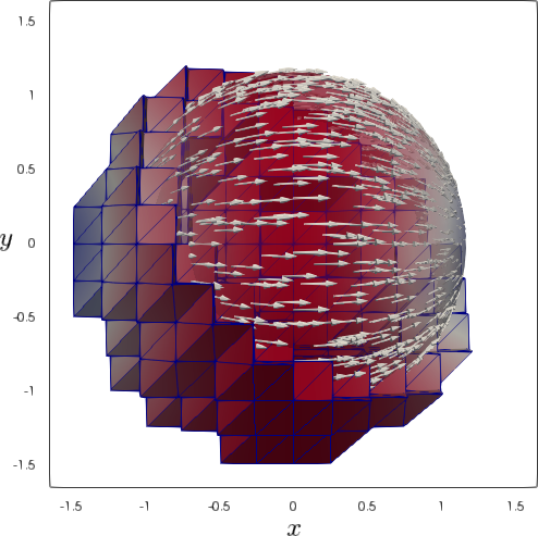
6.2 Tangential flow on a deforming sphere

In this numerical example we consider a deforming unit sphere and compute the induced tangential flow, i.e., the numerical solution of the TSNSE (2.12). Denote by Γ0\Gamma_{0} the reference sphere of radius 11 with the center in the origin OO. Consider spherical coordinates (r,θ,φ)(0,)×[0,π]×[0,2π)(r,\theta,\varphi)\in(0,\infty)\times[0,\pi]\times[0,2\pi) and denote by nm(θ,φ)\mathcal{H}_{n}^{m}(\theta,\varphi), the spherical harmonic of degree nn and order mm. Assume that nm\mathcal{H}_{n}^{m} are normalized, i.e. nmL2(Γ0)=1\|\mathcal{H}_{n}^{m}\|_{L^{2}(\Gamma_{0})}=1. For the evolving surface we consider as ansatz

Γ(t)={𝐱=(r,θ,φ)|r=1+n=1N|m|nAn,m(t)nm(θ,φ)},\Gamma(t)=\left\{\,\mathbf{x}=(r,\theta,\varphi)~{}|~{}r=1+\sum_{n=1}^{N}\sum_{|m|\leq n}A_{n,m}(t)\mathcal{H}_{n}^{m}(\theta,\varphi)\,\right\}, (6.3)

with suitably chosen coefficients An(t)A_{n}(t). The function ξ:=n=1N|m|nAn,m(t)nm(θ,φ)\xi:=\sum_{n=1}^{N}\sum_{|m|\leq n}A_{n,m}(t)\mathcal{H}_{n}^{m}(\theta,\varphi) describes the radial deformation. We assume small oscillations, ξ1\|\xi\|\ll 1. Under this assumption, an accurate approximation of the normal velocity is given by 𝐰N=wN𝐧\mathbf{w}_{N}=w_{N}\mathbf{n}, with

wN=dξdt=n=1N|m|ndAn,mdtnm,𝐧(𝐱)=𝐱/|𝐱|.w_{N}=\frac{d\xi}{dt}=\sum_{n=1}^{N}\sum_{|m|\leq n}\frac{dA_{n,m}}{dt}\mathcal{H}_{n}^{m},\quad\mathbf{n}(\mathbf{x})=\mathbf{x}/|\mathbf{x}|. (6.4)

We want the surface to be inextensible, i.e., ddt|Γ(t)|=0\frac{d}{dt}|\Gamma(t)|=0. Appropriate coefficients An,m(t)A_{n,m}(t) such that we have inextensibility can be determined as follows. Application of the surface Reynolds transport formula and integration by parts gives for the variation of surface area:

ddt|Γ(t)|=ddtΓ(t)1𝑑s=Γ(t)divΓ𝐰N𝑑s=Γ(t)κwN𝑑s.\frac{d}{dt}|\Gamma(t)|=\frac{d}{dt}\int_{\Gamma(t)}1\,ds=\int_{\Gamma(t)}\mbox{div}_{\Gamma}\mathbf{w}_{N}\,ds=\int_{\Gamma(t)}\kappa w_{N}\,ds. (6.5)

For the doubled mean curvature we have, cf. [21],

κ\displaystyle\kappa =22ξΔΓξ=2n=1N|m|n{2An,mnmn(n+1)An,mnm}\displaystyle={2}-{2\xi}-\Delta_{\Gamma}\xi={2}-\sum_{n=1}^{N}\sum_{|m|\leq n}\left\{{2A_{n,m}\mathcal{H}_{n}^{m}}-{n(n+1)}A_{n,m}\mathcal{H}_{n}^{m}\right\}
=2+n=1N|m|nAn,m(n(n+1)2)nm.\displaystyle={2}+\sum_{n=1}^{N}\sum_{|m|\leq n}{A_{n,m}}(n(n+1)-2)\mathcal{H}_{n}^{m}.

Using Γ0nm=0\int_{\Gamma_{0}}\mathcal{H}_{n}^{m}=0, n1n\geq 1, and Γ0nmnm=δnnδmm\int_{\Gamma_{0}}\mathcal{H}_{n}^{m}\mathcal{H}_{n^{\prime}}^{m^{\prime}}=\delta_{n}^{n^{\prime}}\delta_{m}^{m^{\prime}}, we compute for the area variation:

ddt|Γ(t)|=Γ(t)κwN𝑑s=n=1N|m|n(n1)(n+2)dAn,mdtAn,m.\frac{d}{dt}|\Gamma(t)|=\int_{\Gamma(t)}\kappa w_{N}ds=\sum_{n=1}^{N}\sum_{|m|\leq n}{(n-1)(n+2)}\frac{dA_{n,m}}{dt}A_{n,m}. (6.6)

Based on this formula we set A2,0=ϵ2cos(ωt)A_{2,0}=\frac{\epsilon}{2}\cos(\omega t), A3,0=ϵ10sin(ωt)A_{3,0}=\frac{\epsilon}{\sqrt{10}}\sin(\omega t), and An,m=0A_{n,m}=0 for other coefficients. For this choice of coefficients one easily verifies ddt|Γ(t)|=0\frac{d}{dt}|\Gamma(t)|=0. The TSNSE equations (2.12) are then solved with the right hand side given by (2.13) with uN=wNu_{N}=w_{N} computed from (6.4). The initial velocity is zero.
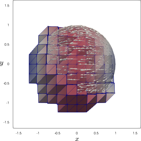
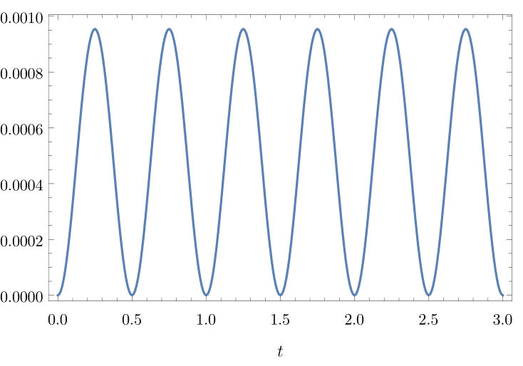
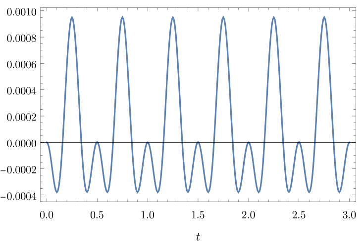
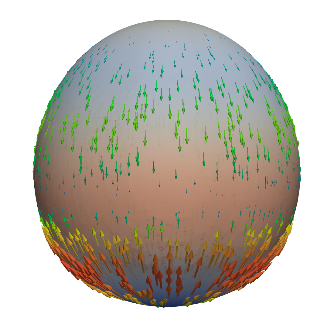
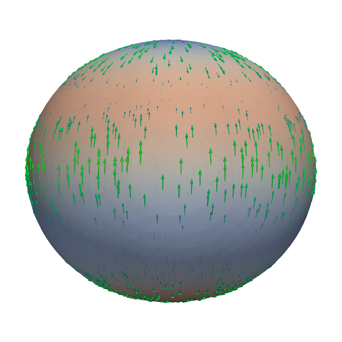
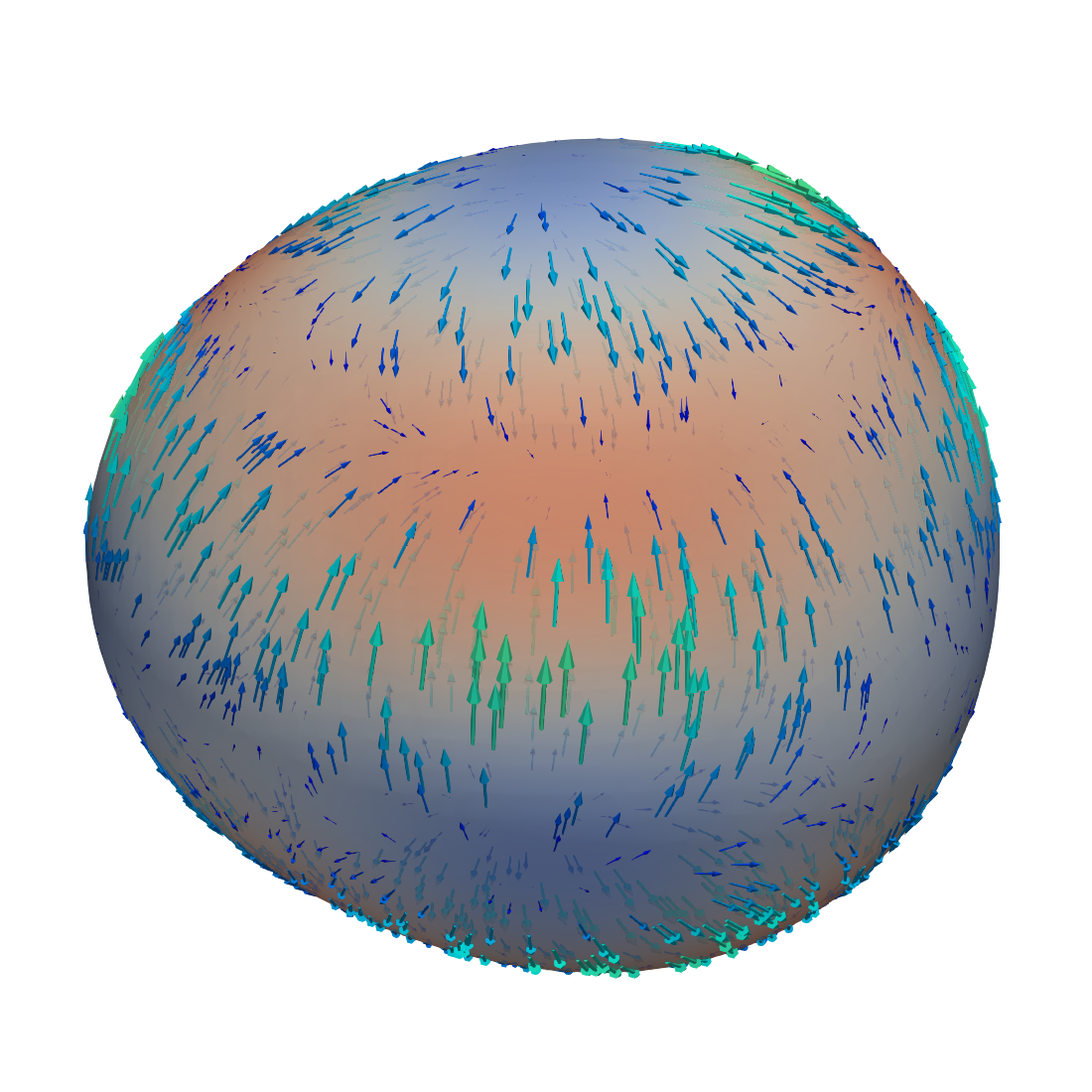
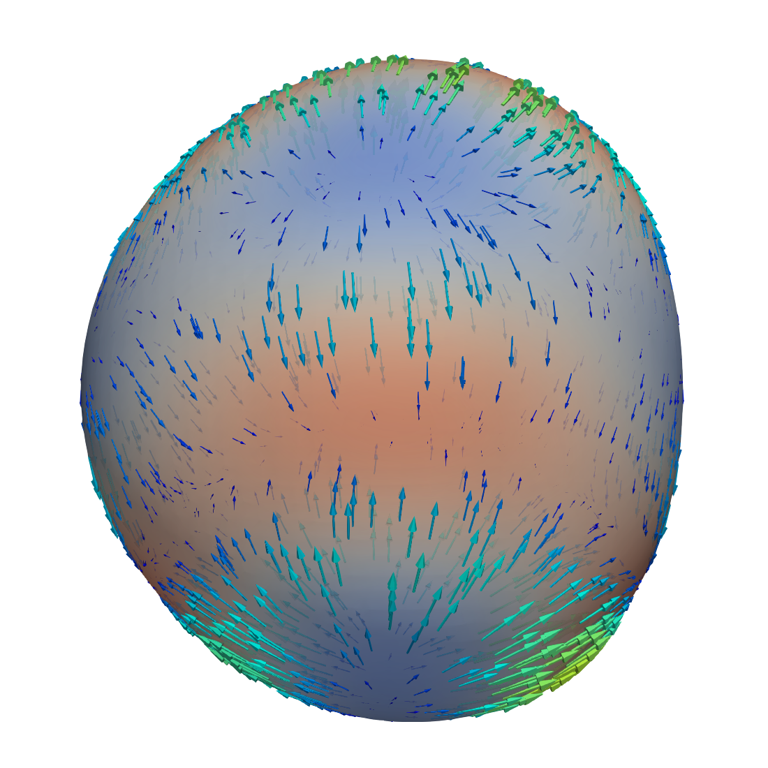
In the first numerical example we let ϵ=0.2\epsilon=0.2, ω=2π\omega=2\pi, μ=12104\mu=\frac{1}{2}10^{-4}, and include 20\mathcal{H}_{2}^{0} and 30\mathcal{H}_{3}^{0}, two zonal spherical harmonics of degree 2 and 3. The relative variation of the surface area Γ(t)\Gamma(t) in the left plot in Figure 2 shows less than 0.1%0.1\% of surface variation, which is due to approximation errors and finite (rather than infinitesimal) deformations. The latter causes an approximation error in (6.4).

Refer to caption
Refer to caption
Fig. 2: Relative surface area variation |Γ(0)||Γ(t)||Γ(0)|\frac{|\Gamma(0)|-|\Gamma(t)|}{|\Gamma(0)|} as a function of time for axisymmetric (left plot) and asymmetric (right plot) deformations of the sphere.

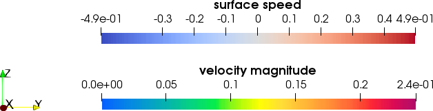
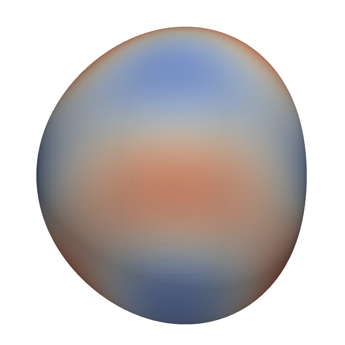
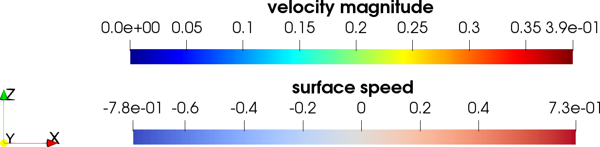
The velocity field induced by these axisymmetric deformations of the sphere is visualized in Figure 3. We see that the velocity pattern is dominated by a sink-and-source flow driven by the term κwN-\kappa w_{N} on the right-hand side of the divergence condition in (2.12).

t=0t=0 Refer to caption

t=0.1t=0.1 Refer to caption

t=0.3t=0.3 Refer to caption

t=0.5t=0.5 Refer to caption

t=0.7t=0.7 Refer to caption

t=0.9t=0.9 Refer to caption

t=1t=1 Refer to caption

Refer to caption
Fig. 3: Visualization of velocity field for axisymmetric deformations of the sphere ; mesh level =4\ell=4, Δt=0.01\Delta t=0.01. Click here to see the full animation.

t=0t=0 Refer to caption

t=0.1t=0.1 Refer to caption

t=0.3t=0.3 Refer to caption

t=0.5t=0.5 Refer to caption

t=0.7t=0.7 Refer to caption

t=0.9t=0.9 Refer to caption

t=1t=1 Refer to caption

Refer to caption
Fig. 4: Visualization of velocity field for asymmetric deformations of the sphere ; mesh level =4\ell=4, Δt=0.01\Delta t=0.01. Click here to see the full animation.

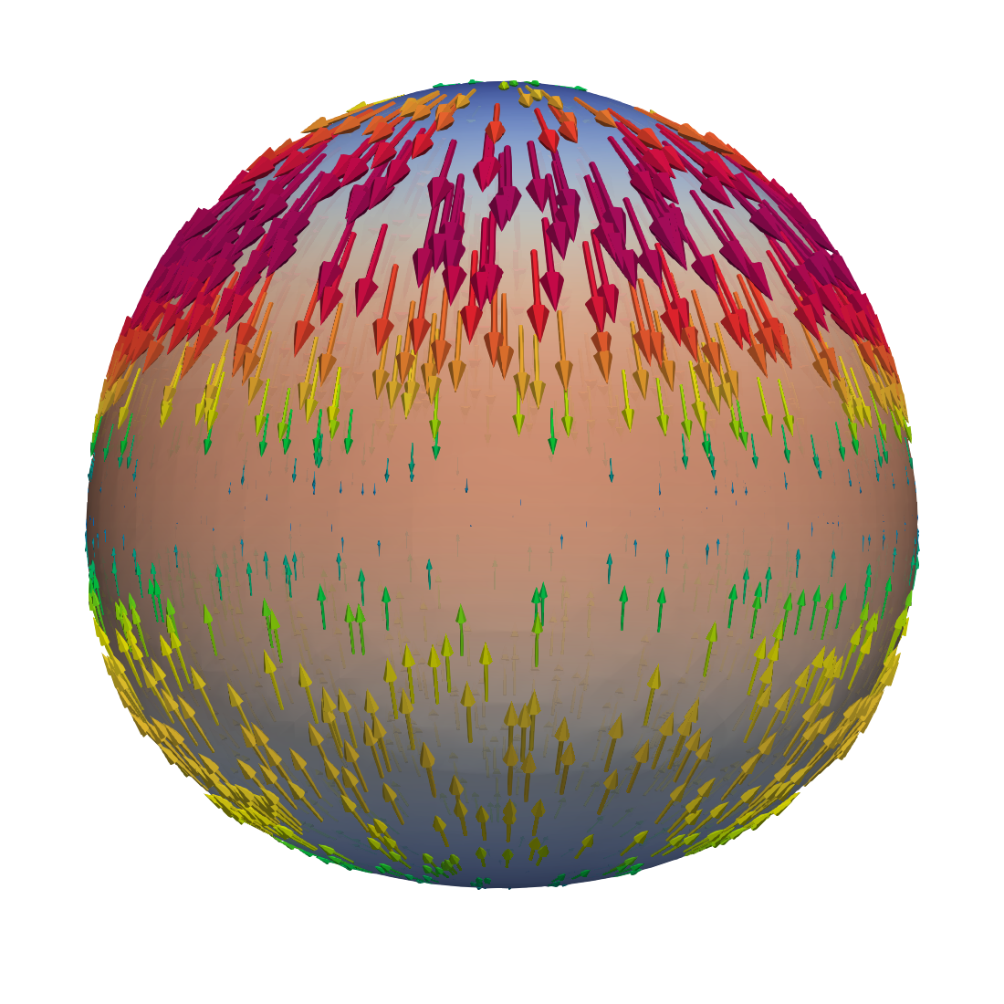
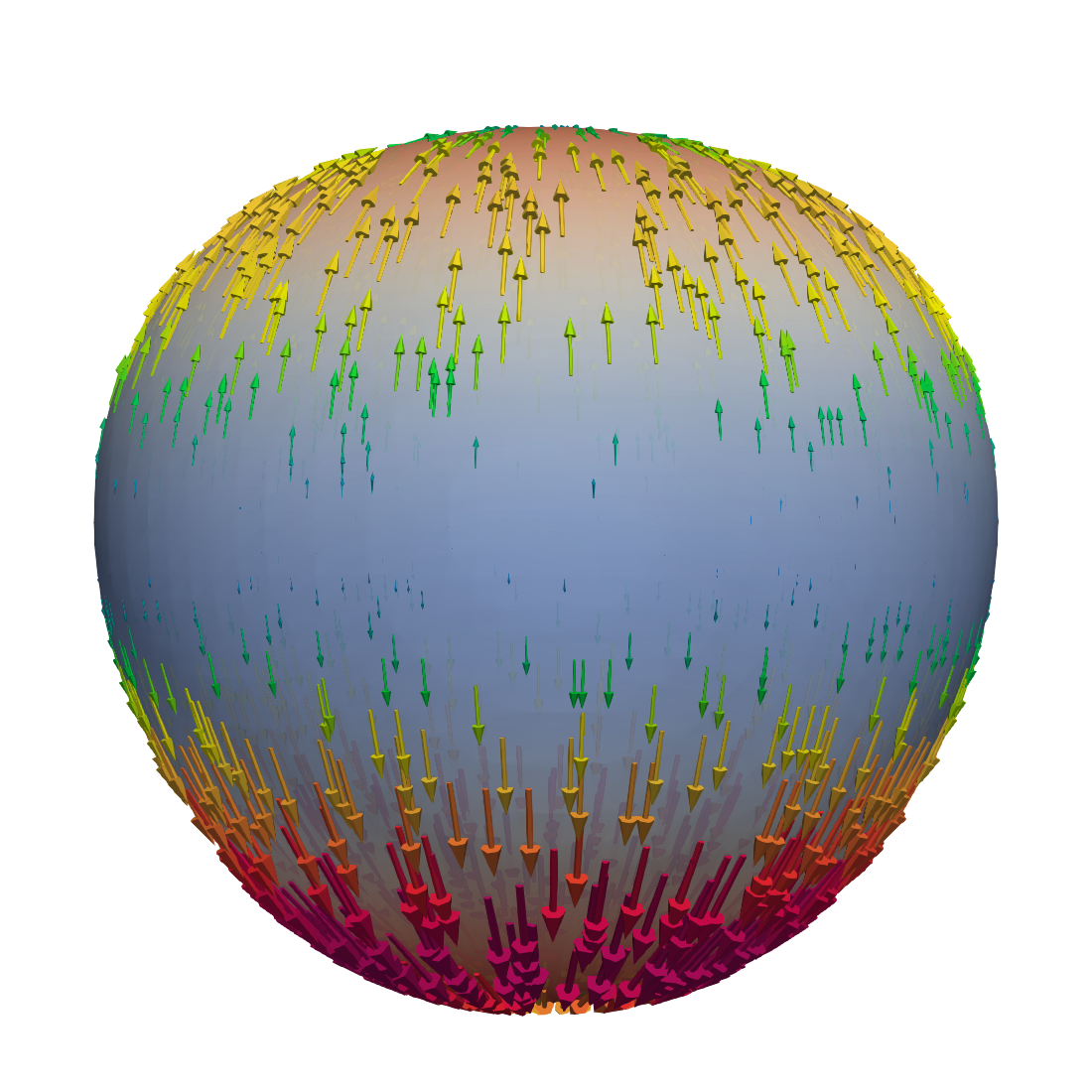
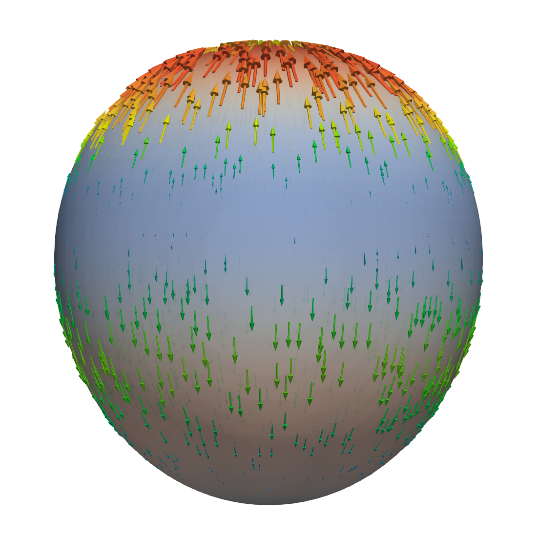
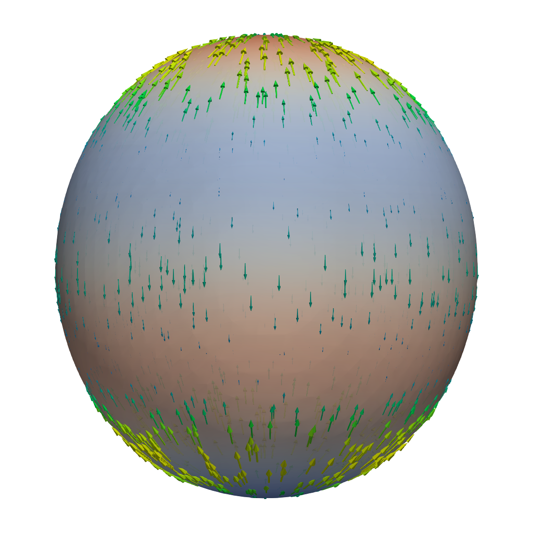
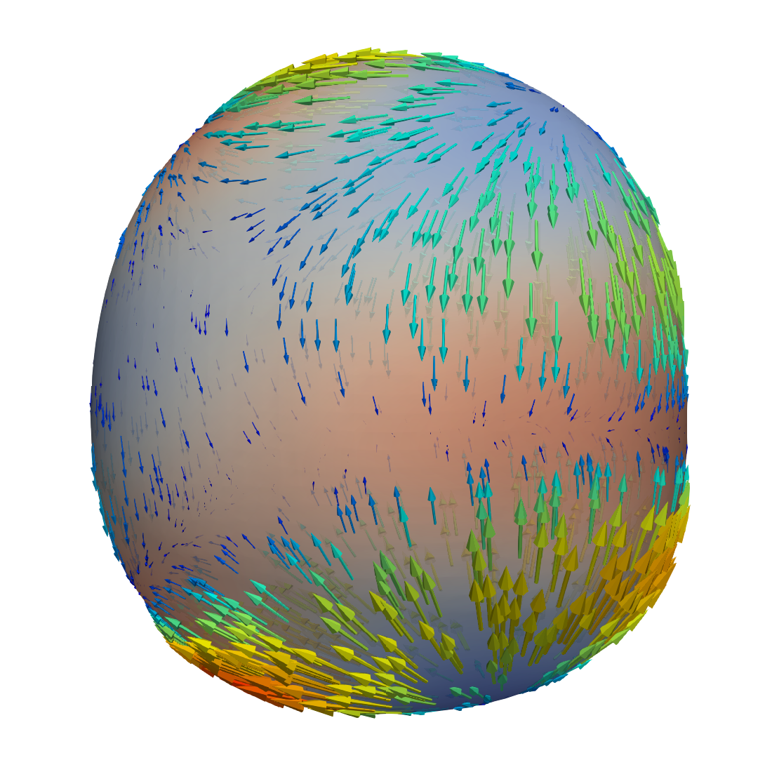
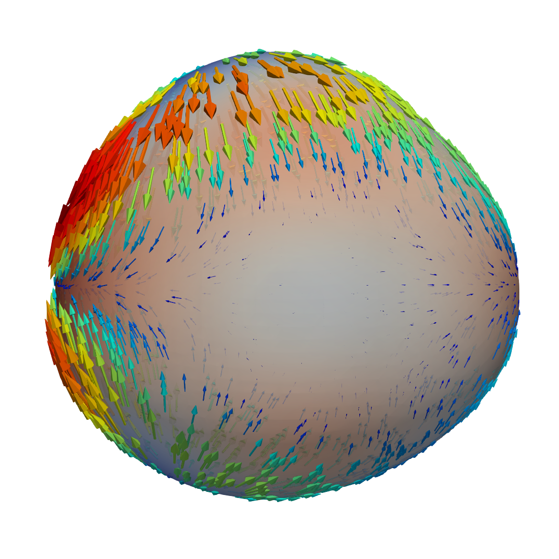
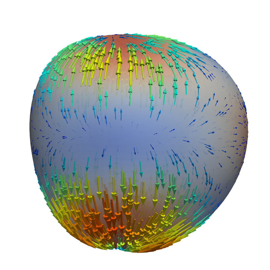
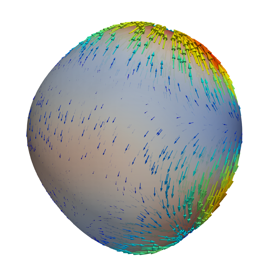
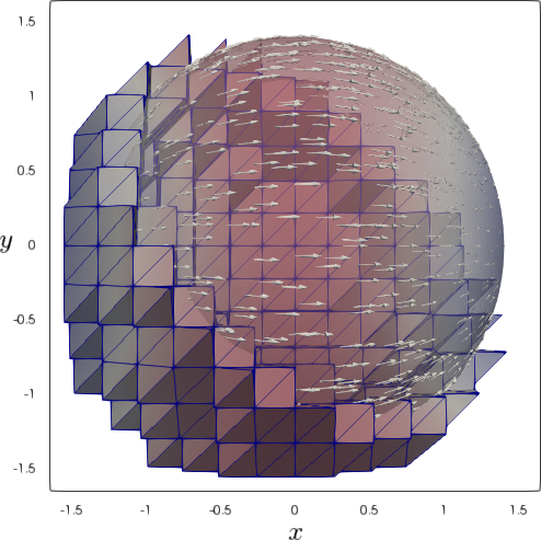
We repeat the experiment, but decrease the viscosity to μ=12105\mu=\frac{1}{2}10^{-5} and add two more spherical harmonics, the sectorial 31\mathcal{H}_{3}^{1} harmonic and the tesseral 42\mathcal{H}_{4}^{2} one, to make the deformation asymmetric. The radial displacement in this experiment is then given by

ξ=0.2(12cos(2πt)20(𝐱)+110sin(2πt)30(𝐱)),+0.1(12cos(4πt)31(𝐱)+518sin(4πt)42(𝐱)).\begin{split}\xi&=0.2\left(\tfrac{1}{2}\cos(2\pi\,t)\,\mathcal{H}_{2}^{0}(\mathbf{x})+\tfrac{1}{\sqrt{10}}\sin(2\pi\,t)\,\mathcal{H}_{3}^{0}(\mathbf{x})\right),\\ &+0.1\left(\tfrac{1}{2}\cos(4\pi\,t)\,\mathcal{H}_{3}^{1}(\mathbf{x})+\tfrac{5}{18}\sin(4\pi\,t)\,\,\mathcal{H}_{4}^{2}(\mathbf{x})\right).\end{split}

Again, the coefficients are such that ddt|Γ(t)|=0\frac{d}{dt}|\Gamma(t)|=0 according to equation (6.6). The resulting velocity field is visualized in Figure 4. The velocity pattern is still dominated by the sink-and-source flow. Note that in both cases there are no outer forces and the flow is completely “geometry driven”.

References

  • [1] A. Alphonse, C. M. Elliott, and B. Stinner, An abstract framework for parabolic PDEs on evolving spaces, Port. Math., (2015), pp. 1–46.
  • [2] V. Arnold, Sur la géométrie différentielle des groupes de lie de dimension infinie et ses applications à l’hydrodynamique des fluides parfaits, in Annales de l’institut Fourier, vol. 16, 1966, pp. 319–361.
  • [3] T. Aubin, Nonlinear analysis on manifolds. Monge-Ampere equations, Springer, Berlin, 1982.
  • [4] J. W. Barrett, H. Garcke, and R. Nürnberg, Numerical computations of the dynamics of fluidic membranes and vesicles, Physical review E, 92 (2015), p. 052704.
  • [5] A. Bonito, A. Demlow, and M. Licht, A divergence-conforming finite element method for the surface Stokes equation, SIAM Journal on Numerical Analysis, 58 (2020), pp. 2764–2798.
  • [6] P. Brandner, A. Reusken, and P. Schwering, On derivations of evolving surface Navier-Stokes equations, arXiv preprint arXiv:2110.14262, (2021).
  • [7] E. Burman, P. Hansbo, M. G. Larson, and A. Massing, Cut finite element methods for partial differential equations on embedded manifolds of arbitrary codimensions, ESAIM: Mathematical Modelling and Numerical Analysis, 52 (2018), pp. 2247–2282.
  • [8] C. Chan, M. Czubak, and M. Disconzi, The formulation of the Navier-Stokes equations on Riemannian manifolds, J. Geom. Phys., 121 (2017), pp. 335–346.
  • [9] G. Dziuk and C. Elliott, Finite elements on evolving surfaces, IMA J. Numer. Anal., 27 (2007), pp. 262–292.
  • [10] G. Dziuk and C. M. Elliott, Finite element methods for surface PDEs, Acta Numerica, 22 (2013), pp. 289–396.
  • [11] D. G. Ebin and J. Marsden, Groups of diffeomorphisms and the motion of an incompressible fluid, Annals of Mathematics, 92 (1970), pp. 102–163.
  • [12] J. Grande, C. Lehrenfeld, and A. Reusken, Analysis of a high-order trace finite element method for PDEs on level set surfaces, SIAM Journal on Numerical Analysis, 56 (2018), pp. 228–255.
  • [13] M. E. Gurtin and A. I. Murdoch, A continuum theory of elastic material surfaces, Archive for Rational Mechanics and Analysis, 57 (1975), pp. 291–323.
  • [14] P. Hansbo, M. G. Larson, and K. Larsson, Analysis of finite element methods for vector Laplacians on surfaces, IMA J. Numer. Anal., (2019).
  • [15] P. Hartman, Ordinary Differential Equations, vol. 590, John Wiley and Sons, 1964.
  • [16] T. Jankuhn, M. A. Olshanskii, and A. Reusken, Incompressible fluid problems on embedded surfaces: Modeling and variational formulations, Interfaces and Free Boundaries, 20 (2018), pp. 353–377.
  • [17] T. Jankuhn, M. A. Olshanskii, A. Reusken, and A. Zhiliakov, Error analysis of higher order trace finite element methods for the surface Stokes equations, Journal of Numerical Mathematics, 29 (2021), pp. 245–267.
  • [18] T. Jankuhn and A. Reusken, Higher order trace finite element methods for the surface Stokes equation, Preprint arXiv:1909.08327, (2019).
  • [19]  , Trace finite element methods for surface vector-Laplace equations, IMA Journal of Numerical Analysis, 41 (2020), pp. 48–83.
  • [20] H. Koba, C. Liu, and Y. Giga, Energetic variational approaches for incompressible fluid systems on an evolving surface, Quarterly of Applied Mathematics, (2016).
  • [21] H. Lamb, Hydrodynamics, University Press, 1924.
  • [22] C. Lehrenfeld and M. Olshanskii, An Eulerian finite element method for PDEs in time-dependent domains, ESAIM: M2AN, 53 (2019), pp. 585–614.
  • [23] C. Lehrenfeld, M. A. Olshanskii, and X. Xu, A stabilized trace finite element method for partial differential equations on evolving surfaces, SIAM Journal on Numerical Analysis, 56 (2018), pp. 1643–1672.
  • [24] T.-H. Miura, On singular limit equations for incompressible fluids in moving thin domains, Quart. Appl. Math., 76 (2018), pp. 215–251.
  • [25] A. Murdoch and H. Cohen, Symmetry considerations for material surfaces, Archive for Rational Mechanics and Analysis, 72 (1979), pp. 61–98.
  • [26] I. Nitschke, S. Reuther, and A. Voigt, Hydrodynamic interactions in polar liquid crystals on evolving surfaces, Phys. Rev. Fluids, 4 (2019), p. 044002.
  • [27] M. Olshanskii, A. Reusken, and J. Grande, A finite element method for elliptic equations on surfaces, SIAM J. Numer. Anal., 47 (2009), pp. 3339–3358.
  • [28] M. Olshanskii, A. Reusken, and A. Zhiliakov, Inf-sup stability of the trace P2-P1 Taylor–Hood elements for surface PDEs, Mathematics of Computation, 90 (2021), pp. 1527–1555.
  • [29] M. A. Olshanskii, A. Quaini, A. Reusken, and V. Yushutin, A finite element method for the surface Stokes problem, SIAM Journal on Scientific Computing, 40 (2018), pp. A2492–A2518.
  • [30] M. A. Olshanskii and A. Reusken, Trace finite element methods for PDEs on surfaces, in Geometrically Unfitted Finite Element Methods and Applications, S. P. A. Bordas, E. Burman, M. G. Larson, and M. A. Olshanskii, eds., Cham, 2017, Springer International Publishing, pp. 211–258.
  • [31] M. A. Olshanskii, A. Reusken, and X. Xu, An Eulerian space–time finite element method for diffusion problems on evolving surfaces, SIAM Journal on Numerical Analysis, 52 (2014), pp. 1354–1377.
  • [32] M. A. Olshanskii and V. Yushutin, A penalty finite element method for a fluid system posed on embedded surface, Journal of Mathematical Fluid Mechanics, 21 (2019), p. 14.
  • [33] J. Prüss, G. Simonett, and M. Wilke, On the Navier-Stokes equations on surfaces, J. Evol. Equ., 21 (2021), pp. 3153–3179.
  • [34] P. Rangamani, A. Agrawal, K. K. Mandadapu, G. Oster, and D. J. Steigmann, Interaction between surface shape and intra-surface viscous flow on lipid membranes, Biomechanics and modeling in mechanobiology, (2013), pp. 1–13.
  • [35] A. Reusken, Stream function formulation of surface Stokes equations, IMA Journal of Numerical Analysis, 40 (2020), pp. 109–139.
  • [36] S. Reuther and A. Voigt, The interplay of curvature and vortices in flow on curved surfaces, Multiscale Modeling & Simulation, 13 (2015), pp. 632–643.
  • [37]  , Erratum: The interplay of curvature and vortices in flow on curved surfaces, Multiscale Modeling & Simulation, 16 (2018), pp. 1448–1453.
  • [38]  , Solving the incompressible surface Navier–Stokes equation by surface finite elements, Physics of Fluids, 30 (2018), p. 012107.
  • [39] P. Saffman and M. Delbrück, Brownian motion in biological membranes, Proceedings of the National Academy of Sciences, 72 (1975), pp. 3111–3113.
  • [40] G. Simonett and M. Wilke, HH^{\infty}-calculus for the surface Stokes operator and applications, arXiv preprint arXiv:2111.12586, (2021).
  • [41] P. Steinmann, On boundary potential energies in deformational and configurational mechanics, Journal of the Mechanics and Physics of Solids, 56 (2008), pp. 772–800.
  • [42] M. E. Taylor, Analysis on Morrey spaces and applications to Navier-Stokes and other evolution equations, Communications in Partial Differential Equations, 17 (1992), pp. 1407–1456.
  • [43] R. Temam, Navier–Stokes equations, theory and numerical analysis, North-Holland, Amsterdam, 1977.
  • [44]  , Infinite-dimensional dynamical systems in mechanics and physics, Springer, New York, 1988.
  • [45] A. Torres-Sánchez, D. Millán, and M. Arroyo, Modelling fluid deformable surfaces with an emphasis on biological interfaces, Journal of Fluid Mechanics, 872 (2019), pp. 218–271.
  • [46] H. von Wahl, T. Richter, and C. Lehrenfeld, An unfitted Eulerian finite element method for the time-dependent Stokes problem on moving domains, IMA Journal of Numerical Analysis, (2021).
  • [47] A. Yavari, A. Ozakin, and S. Sadik, Nonlinear elasticity in a deforming ambient space, J. Nonlinear Sci., 26 (2016), pp. 1651–1692.