Task and Configuration Space Compliance of
Continuum Robots via Lie Group and Modal Shape Formulations
Abstract
Continuum robots suffer large deflections due to internal and external forces. Accurate modeling of their passive compliance is necessary for accurate environmental interaction, especially in scenarios where direct force sensing is not practical. This paper focuses on deriving analytic formulations for the compliance of continuum robots that can be modeled as Kirchhoff rods. Compared to prior works, the approach presented herein is not subject to the constant-curvature assumptions to derive the configuration space compliance, and we do not rely on computationally-expensive finite difference approximations to obtain the task space compliance. Using modal approximations over curvature space and Lie group integration, we obtain closed-form expressions for the task and configuration space compliance matrices of continuum robots, thereby bridging the gap between constant-curvature analytic formulations of configuration space compliance and variable curvature task space compliance. We first present an analytic expression for the compliance of a single Kirchhoff rod. We then extend this formulation for computing both the task space and configuration space compliance of a tendon-actuated continuum robot. We then use our formulation to study the tradeoffs between computation cost and modeling accuracy as well as the loss in accuracy from neglecting the Jacobian derivative term in the compliance model. Finally, we experimentally validate the model on a tendon-actuated continuum segment, demonstrating the model’s ability to predict passive deflections with error below 11.5% percent of total arc length.
I Introduction
In this paper, we consider how to compute the passive compliance matrix of continuum and soft robots modeled as Kirchhoff rods (i.e. Cosserat rods with negligible shear strains and extension). The local compliance matrix provides a local prediction of the robot’s passive deflections as a result of small changes in external loads, so it is useful for design and planning to ensure accurate physical interaction with the environment. The compliance matrix also needs to be computed for online passive stiffness modulation [1, 2, 3] and active stiffness/compliant motion control [4, 5, 6].
Many prior works presented mechanics models to predict the overall deflection of a continuum or soft robot for a given set of actuation and external loads [7, 8, 9]. However, relatively few studied the local compliance, i.e. the small change in shape due to small changes in the applied forces [10, 11, 6, 12]. These prior works on local compliance have defined the compliance matrix in two different ways: configuration space or task space compliance, depending on the application need.
The configuration space compliance relates external wrenches projected into the robot’s configuration space to the ensuing changes in the configuration variables. This notion of compliance was used in [6] for compliant motion control, in [13, 14] for force regulation without dedicated end-effector force sensing, and in [15] for force-controlled shape scanning of organs. Configuration space compliance can be computed analytically, but prior work has only presented it under the assumption of a constant-curvature shape.
The task space compliance is the more conventional notion of compliance that provides the twist that a robot experiences as a result of a small change in an applied external wrench. While using finite differences to compute this compliance is possible, this approach is computationally expensive and does not provide analytic expressions of the compliance. Another method, applied to a concentric tube robot in [11], integrates an additional set of differential equations together with the standard Cosserat rod equations. This can be combined with finite difference steps to compute the compliance matrix of a parallel continuum robot[12]. In the mechanics literature, variational formulations were also used to derive stiffness matrices for geometrically exact mechanics models [16, 17], but these methods have not been translated into a robotics context. Finally, [10] presented the task-space compliance of a continuum segment with discrete actuators applying moment loads along the segment’s body. This work used modal basis functions to describe the backbone bending angle, resulting in an analytic expression for the task-space compliance, but it was limited to planar deflections.
The contribution of this paper is a compliance matrix formulation that bridges the gap between constant-curvature configuration space compliance and geometrically-exact task space compliance. We present analytic expressions for both configuration and task space compliance. The analytic nature of the formulation enables sensitivity analysis of individual model parameters on the resulting configuration. As an example, we show how the term associated with the derivatives of the task space Jacobian and the external loading has a significant effect on the accuracy of the compliance model. We also show how our approach enables a tradeoff to be made to between model accuracy and computation cost, which is more difficult to achieve using prior geometrically exact mechanics models.
In Section II, we present the kinematic equations describing the variable curvature kinematic shape of the robot. In Section III, we then show how to derive the task space compliance of a single Kirchhoff rod from the modal shape kinematics and local rod stiffness. We then extend this to the task space and configuration space compliance of a tendon-actuated continuum segment in Section IV. Finally, in Section V, we present a simulation case study of a single Kirchhoff rod and an experimental validation of the compliance matrix on a tendon-actuated continuum segment.
II Lie Group Kinematics Preliminaries
In this section, we summarize the kinematic expressions that underpin our proposed compliance matrix formulation in this paper. The Lie group kinematics was presented in [18] as part of a formulation for continuum robot shape estimation from intrinsic string encoder measurements. Prior works have used modal shape functions to model hyper-redundant [19] and continuum/soft robots [20, 21, 22, 23, 24, 25], but the kinematic expressions presented herein are most similar to those used in [26, 27] for continuum robot mechanics, where the modal shape functions approximate the local backbone curvature.
II-A Central Backbone Kinematics
Referring to Fig. 1, we define the arc length distance along the central backbone as , where is the total length of the central backbone. We also assume the central backbone has a high slenderness ratio consistent with the assumption of negligible shear strains, i.e. a Kirchhoff rod. The central backbone can therefore be described by the curvature distribution along the backbone in three directions, . At a given arc length , we assign a local body frame with its z-axis tangent to the central backbone curve:
| (1) |
where and are the orientation111We use the notation to denote the orientation of frame {A} with respect to frame {B}. Also, frame {A} has its origin denoted by . of the local body frame in the base frame {0} and the position of the origin of frame {T} in frame {0}. As the body frame traverses the central backbone curve, it undergoes a twist , where denotes the local tangent unit vector. Furthermore, it satisfies the following differential equation [28]:
| (2) |
where denotes the derivative with respect to and the hat operator forms the standard matrix representations of and from the vector forms and , respectively.
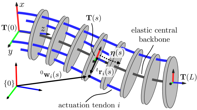
We now make a choice to express the curvature distribution as a weighted sum of polynomial functions. We denote the polynomial functions as , , and and the weights as , , and , for the , , and directions, respectively. The curvature is therefore:
| (3) |
where the columns of form a modal shape basis, and is a vector of constant modal coefficients.
We choose the Chebyshev polynomials of the first kind for the modal functions since their roots are also the Chebyshev nodes, resulting in optimal approximation. They can be computed recursively:
| (4) |
where we shift the domain to via the transformation . The benefit of this modal shape approach to modeling the kinematics of continuum robots is that variable curvature shapes with any desired choice of fidelity can be modeled by a suitable choice of the modal shape basis order. We will show below how this approach bridges the gap between prior constant-curvature configuration-space compliance and Kirchhoff rod task-space compliance models.
For a given configuration , the body frame is found by integrating (2). As reviewed in [29], a variety of Lie group integration methods could be used for this, including an approach based on the Magnus expansion that we use here, following our result in [30]. After integrating (2), the spatial curve is given via a product of matrix exponentials:
| (5) |
where the particular form of depends on the choice of integration method [29, 30].
II-B Tendon Routing Kinematics
To model the kinematics of the tendon paths, we follow the approach used in [31]. Assuming tendons, the tendon path is expressed in the moving frame and is given by:
| (6) |
The position of a point along the tendon path is given in the world frame by:
| (7) |
Noting that vector norms are invariant under rotations, the length of the tendon is therefore given by:
| (8) |
where is the central backbone arc length at which the tendon is anchored to the spacer disk/end disk, and is found by taking the derivative of (7) with respect to and substituting (3), , and :
| (9) |
II-C Instantaneous Kinematics Jacobians
Using the equations above, we also define two instantaneous kinematics Jacobians that will be used to formulate the configuration space and task space compliance matrices. Noting that the vector of modal coefficients uniquely defines the configuration of the robot, we define the configuration space Jacobian as the Jacobian relating small changes in the tendon lengths to small changes in the modal coefficients:
| (10) |
III Compliance Matrix of a Kirchhoff Rod
We now build on the kinematic equations above to formulate the compliance matrix of a Kirchhoff rod. We follow a similar set of steps as the derivation of the stiffness matrix for a parallel robot in [1] and the statics [32] and stiffness of multi-backbone robots [6]. We begin by defining a small perturbation (i.e. a twist) in the end effector pose , denoted as , which we find by computing the body twist and then transforming into the hybrid frame that is coincident with the body frame but aligned with the world frame:
| (12) |
where is the rotation matrix of the body frame expressed in the world frame and the “vee" operator extracts a vector from its corresponding skew-symmetric cross-product matrix . We then define the task-space compliance matrix of a single rod as:
| (13) |
where is a small change in the applied wrench written in the hybrid frame222The hybrid frame has its origin coincident with the origin of the local frame {T} and its axes parallel to the base frame {0}. and with the moment followed by the force.
We assume here the rod is massless, and that shear strains and extension are negligible. We denote as the diagonal bending/torsion stiffness matrix of the rod’s cross section. The bending energy in the rod is given by
| (14) |
where we have substituted the modal shape basis curvature from (3). Note that the matrix can be computed offline if the modal shape functions are chosen a priori.
For the work done by the applied wrench as it produces a small displacement , there is a corresponding small change in bending energy :
| (15) |
Recalling the body Jacobian from (11), we denote the relationship between and as:
| (16) |
and substitute this into (15):
| (17) |
By the principle of virtual work, to be in static equilibrium we require the virtual displacements associated with to vanish, resulting in:
| (18) |
Denoting as the element of and taking small perturbations about the equilibrium configuration:
| (19) |
By substituting and and solving for we obtain:
| (20) |
Recalling (13) and substituting (20) into results in the analytic expression for the compliance matrix:
| (21) |
The above result matches with the congruence transformation of stiffness as discussed in [33] for serial robots. The energy Hessian , which can be computed offline, is found by differentiating (14) twice:
| (22) |
IV Compliance Matrices of a Tendon-actuated Continuum Segment
We now extend the example above for a single rod to the case of a tendon-actuated continuum segment. We first derive a statics model similar to the constant curvature model in [34] but for a variable curvature segment. We then use this statics model to arrive at the task-space compliance matrix, in an analytic form as a result of our Lie group modal shape formulation. Finally, we present the variable curvature configuration-space compliance matrix.
IV-A Task-space compliance
For a given external wrench on the tip of the segment and a perturbation in the end pose, we have a corresponding change in the forces applied to the actuation tendons and a corresponding change in the bending energy stored in the segment, where the bending energy is given by (14). Following the principle of virtual work, we have:
| (23) |
where is a change in the tendon length. Referring to (11) and (10), we substitute (16) and to arrive at the statics of the segment about a given configuration:
| (24) |
We then take small perturbations of this statics expression:
| (25) |
where and are defined as:
| (26) |
| (27) |
The matrix is the contribution to the compliance matrix of the forces on the tendons at the current configuration, and is the contribution due to the external wrench. can be readily affected by using actuation redundancy (internal preload) and depends only on the external load. In a robot without actuation redundancy, is determined by through the statics equation. Therefore and are not completely independent. In a robot with actuation redundancy, these two matrices are independent.
By defining the joint-level stiffness as a diagonal stiffness matrix containing the stiffness of individual actuation lines, i.e., , we can use and in (25), combine like terms, and solve for :
| (28) |
We then substitute this expression into to arrive at the compliance matrix:
| (29) |
As a result of our analytic kinematic expressions, (29) bears resemblance to the results of prior works on stiffness modulation of rigid-link parallel robots, where one defines an active stiffness term dependent on the joint-level forces and the derivative of the Jacobian. and a passive stiffness term dependent on joint-level stiffness [35, 36, 37]. Compared to a rigid-link parallel robot stiffness matrix model, additional terms for tendon-actuated continuum robots include the Hessian of the bending energy and a term with the joint forces multiplied by the derivatives of the configuration-space Jacobian.
IV-B Configuration-space compliance
We now present the configuration space compliance matrix for a tendon-actuated continuum segment with variable curvature deflections. Our formulation can be seen as an extension of the compliance matrix in [6] to the case of variable curvature continuum robots. The resulting expression does not require computation of the task space Jacobian and its derivatives, and is therefore less computationally expensive. Furthermore, it does not require knowledge of the external wrench as required by the task-space compliance, so we believe it can be used for compliant motion control as done in [6], but for cases where large external loads produce variable curvature deflections.
Referring to (24), we first define the external wrench projected into the configuration space, denoted as :
| (30) |
Taking small perturbations of (30) results in
| (31) |
where was given in (25). We now substitute , combine like terms, and solve for :
| (32) |
Computing the change in the configuration for a small change in the projected wrench, i.e. , results in the following configuration-space compliance matrix:
| (33) |
Note that (33) does not require that the task-space Jacobian and its derivatives be computed. It also does not require knowledge of the external wrench. It does, however, in the general case require knowledge of the actuation tendon forces. These forces can come either directly from force sensors placed in series with the actuation tendons [6, 12] or from estimates obtained via the commanded motor current. In special cases where constant, e.g. segments with constant pitch tendon routing and negligible torsional deflections as in Section V, is zero and the actuation tendon forces do not need to be measured.
IV-C Determining the configuration modal coefficients
Both the configuration-space and task-space compliance matrices require the modal coefficients to define the segment’s configuration. There are two ways to obtain . The first is using the shape sensing approach presented in [18]. This approach requires integration of shape-sensing hardware, but the benefit is that it does not require a potentially computationally expensive mechanics model.
The second way to obtain is with a mechanics model like the ones presented in [30, 9]. After solving the mechanics model, can be obtained by converting the collocation values into modal coefficients, as shown in [38]. Using a mechanics model to obtain does not require shape-sensing, but does require an estimate of the external wrench applied to the segment, which may be known a-priori in some cases or can be measured using a load cell attached to the end effector.
V Simulation and Experimental Results
In this section, we present a simulation-based analysis of the Kirchhoff rod compliance matrix model, as well as an experimental validation and analysis of the compliance matrix for a tendon-actuated continuum segment.
V-A Kirchhoff rod model validation and analysis in simulation
We first compare the deflections predicted by our compliance matrix in (21) to the deflections predicted by a Kirchhoff rod model, solved following the method in [38] which combined orthogonal collocation and Lie group integration. We considered a 2 mm diameter Nitinol rod with a length of 200 mm and combinations of 1 N tip forces and 0.5 Nm tip wrenches, generating a set of 2187 rod shapes. For each shape, we applied small steps of 0.1 N and 0.05 Nm to increment the applied force/moment (6 deflections for each shape) and recomputed the Kirchhoff rod model. We then used (21) to predict the deflection for each wrench increment. For (21), we used the same Chebyshev series for the , , and directions, but varied the order of the Chebyshev series from to , i.e. when , had three columns, and when , had 33 columns. We used 10 integration steps when computing regardless of . We then computed the tip translational deflection error:
| (34) |
where is the deflection predicted by the Kirchhoff rod model and is the deflection from (21). The solvers were run using MATLAB 2021a on an Intel i7-11700 CPU.
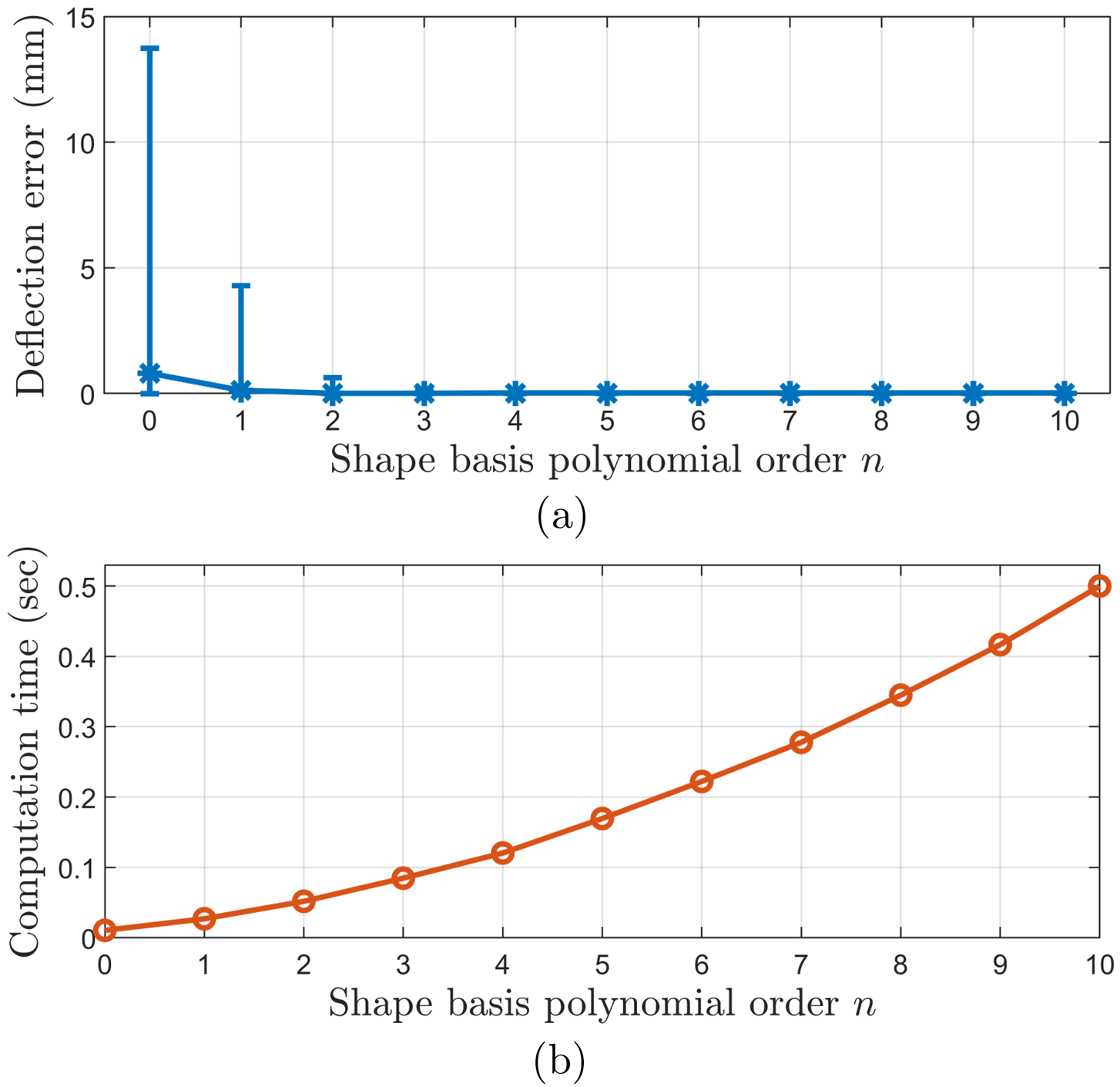
| Position error (mm) | Rotation error (deg) | ||||
|---|---|---|---|---|---|
| Avg. | Max. | Avg. | Max. | Speed (Hz) | |
| 0.8 | 13.7 | 0.2 | 6.3 | 94.6 | |
| 1.3e-2 | 0.6 | 2.2e-3 | 0.10 | 19.3 | |
| 6.7e-5 | 6.3e-3 | 2.0e-5 | 1.2e-3 | 8.3 | |
| 1.5e-5 | 3.8e-4 | 1.3e-5 | 4.4e-4 | 4.5 | |
The mean/max absolute deflection error results are shown in Table I and Fig. 2. We see that as is increased, the analytic expression rapidly converges to the simulated Kirchhoff rod deflection. We also observe that computation time increases with , showing a tradeoff between the compliance matrix accuracy and computation cost.
The primary source of computational cost is in computing the derivatives of . For , estimating these derivatives accounts for approximately 95% of the computation time. We are currently using finite differences to estimate these derivatives, but we believe it is possible to derive these derivatives analytically and reduce computation cost. Methods from [29] to reduce the number of Lie brackets needed to calculate could also reduce computation cost.
A benefit of our formulation, in contrast to other approaches to computing the compliance matrix, is that it allows a trade-off between computation cost and accuracy to be made depending on the application need. A high-order model (large ) to be used when computing the statics model to accurately predict the spatial shape of the continuum robot, but use a lower-order model (small ) to compute the compliance matrix for online compliant motion control or predicting local deflections.
| Position error (mm) | Rotation error (deg) | ||||
|---|---|---|---|---|---|
| Avg. | Max. | Avg. | Max. | Speed (Hz) | |
| 3.23 | 30.5 | 0.94 | 14.3 | 665.3 | |
| 2.82 | 37.1 | 1.05 | 10.1 | 335.0 | |
| 2.83 | 37.1 | 1.06 | 10.2 | 237.0 | |
| 2.83 | 37.1 | 1.06 | 10.2 | 184.8 | |
To reduce computation cost, one may ask whether it is possible to neglect the term that includes the derivatives of the task-space Jacobian and external wrench. While this term is typically negligible for stiff rigid-link robots [39], it was shown in [40] that this term is not negligible for robots with compliant actuators. Here we show a similar result for continuum robots, by computing (21) while neglecting this term using the same set of 2187 rod shapes and increments in wrench described above, and comparing again to the local deflections predicted by the Kirchhoff rod model. The mean absolute position and orientation errors are given in Table. II. We observe that while the speed of computing (21) increases significantly, the maximum position and orientation errors are high when neglecting this term. We also observe that increasing the number of modal coefficients does not significantly improve the modeling error when neglecting the task space Jacobian derivatives.
V-B Experimental validation
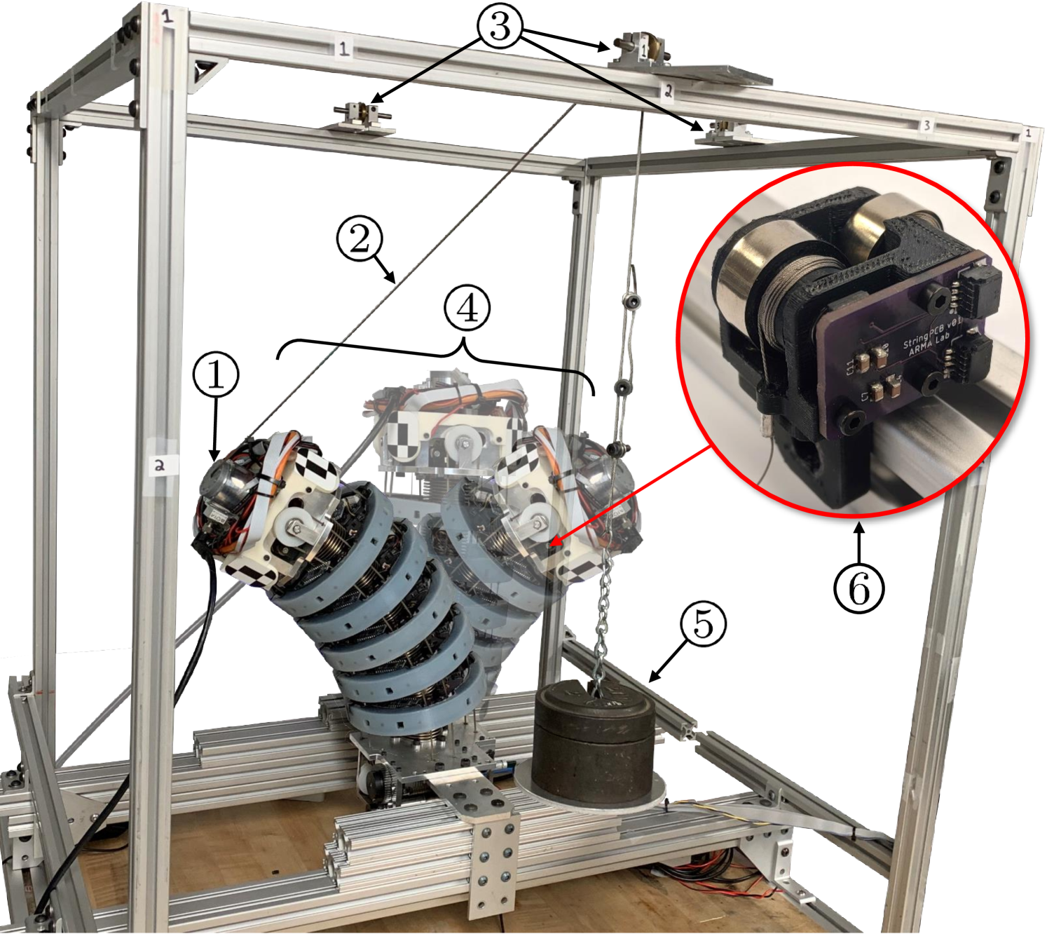
In this section, we describe the experimental validation of our method on a tendon-actuated continuum segment, shown in Fig. 3. The continuum segment central backbone is 300.6 mm in length and the kinematic radius of the actuation tendons is 65.2 mm. Two actuators are integrated into the base, which drive the actuation tendons that bend the segment. In the end-disk are four string encoders that measure the deflections of the segment to estimate . In [18], it was shown that this shape sensing approach, which is purely kinematic and does not require a mechanics model, can estimate the end disk position to within 5% of total arc length, or 14.4 mm of position error.
Metal bellows in the segment’s flexible backbone structure make it approximately 1950 times stiffer in torsion that in bending, so we neglect the torsional deflections and use the following modal shape basis:
| (35) |
where . With this choice of and since the strings and actuaton tendons are routed in constant-pitch radius paths, is constant, and .
| Configuration | 1 | 2 | 3 | 4 | 5 |
|---|---|---|---|---|---|
| 0° | 500° | -500° | 500° | 0° | |
| 500° | 0° | 500° | -500° | 0° |
The experimental setup used to validate the compliance matrix model is shown in Fig. 3. In order to experimentally validate our approach, we attached a force/torque sensor (Bota Systems Rokubi™) to the end effector of the segment. The segment was actuated to five different joint space configurations in the segment’s workspace. The angles of the first and second actuators, denoted as and , respectively, are given in Table III. At each configuration, the unloaded configuration of the segment was measured using the string encoders. A mass was then attached to the force/torque sensor via a wire-rope hung over a pulley. The segment’s new deflected configuration and the applied wrench was then measured. This was repeated for each configuration using 10 different combinations of wire rope direction and masses ranging from 2 lbs to 10 lbs, resulting in a total of 50 measured deflections.
Across the 50 deflections, the mean and maximum deflection was 14.3 mm and 66.7 mm, respectively. The first 10 deflections used for the first joint-space configuration were used to calibrate the model parameters and . We did this by solving for the values of these parameters that minimized the least-squared error between the model predicted deflection and the experimentally measured deflection, solved with lsqnonlin() in MATLAB. The resulting calibrated values were Nm2 and N/m.
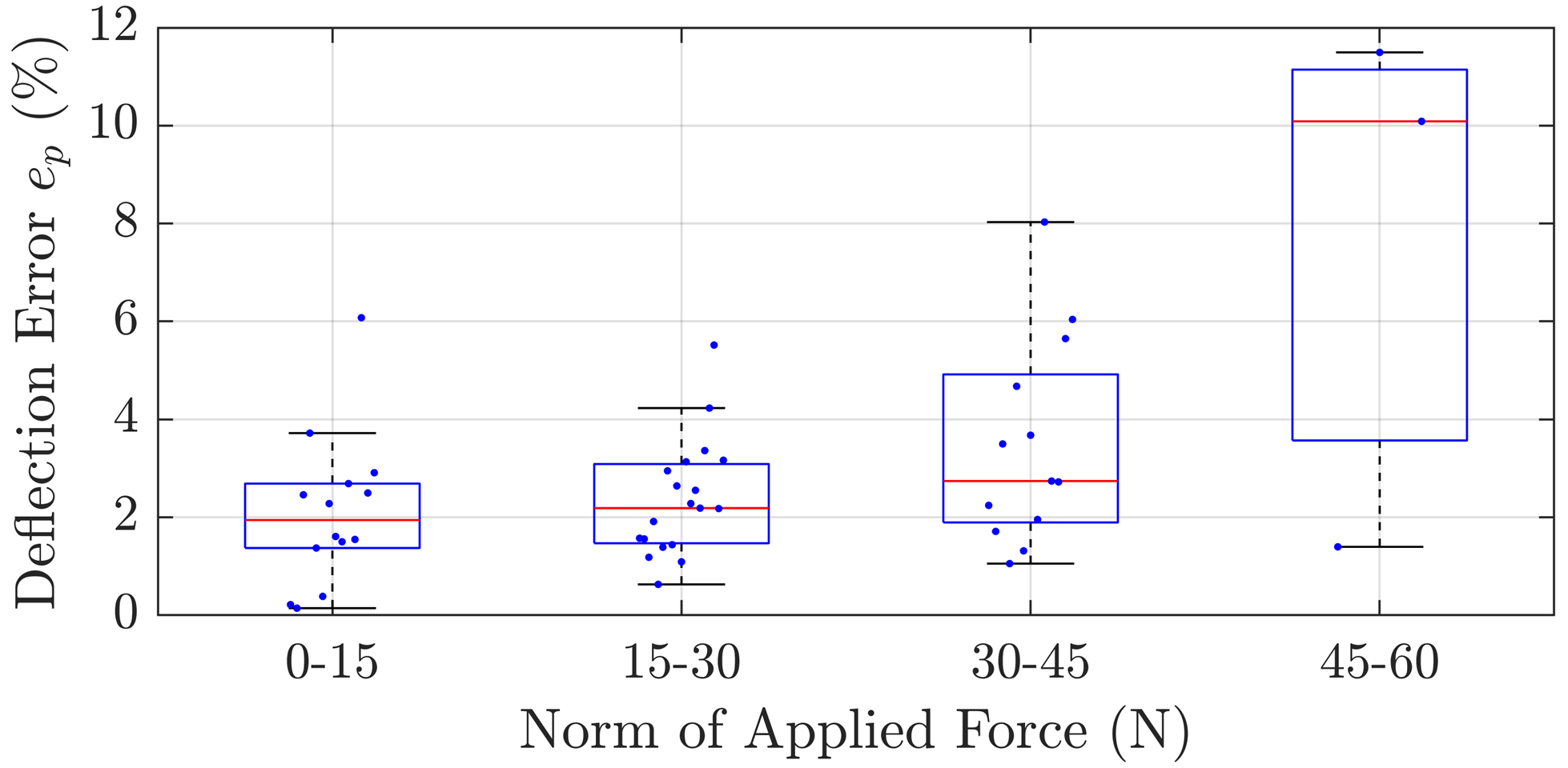
The remaining 40 deflections were used to validate the model. Comparing the measured and model-predicted deflections, the mean and max absolute error from 34 was 9.1 mm and 34.6 mm, respectively, or 3.0% and 11.5% of the backbone length. Since the compliance matrix is only a local estimate of the deflection behavior, it is expected that larger deflections result in larger error in the predicted deflection. Figure 4 shows predicted deflection error for different norms of applied force. We observe that, as expected, predicted deflection error tends to increase as the applied force increases.
VI Conclusions
In this paper, we presented a method for computing the compliance matrix of continuum and soft robots utilizing a modal shape basis Lie group formulation. Compared to prior work, our approach does not rely on a constant-curvature assumption and leads to analytic expressions for both configuration space and task space compliance. We presented the compliance of a single Kirchhoff rod, and we highlighted through a simulation study the tradeoff between computational cost and modeling accuracy as well as the importance of including the Jacobian derivatives when computing compliance. We also presented the compliance for a tendon-actuated continuum segment, and performed an experimental validation of the task-space compliance, showing predicted deflection errors below 11.5% of arc length. Future work includes applying this formulation to passive stiffness modulation and compliant motion control of variable curvature continuum and soft robots.
References
- [1] A. L. Orekhov and N. Simaan, “Directional stiffness modulation of parallel robots with kinematic redundancy and variable stiffness joints,” Journal of Mechanisms and Robotics, vol. 11, no. 5, Jul. 2019.
- [2] J. J. Rice and J. M. Schimmels, “Passive compliance control of redundant serial manipulators,” Journal of Mechanisms and Robotics, vol. 10, no. 4, p. 041009, 2018.
- [3] A. Alamdari, R. Haghighi, and V. Krovi, “Stiffness modulation in an elastic articulated-cable leg-orthosis emulator: Theory and experiment,” IEEE Transactions on Robotics, vol. 34, no. 5, pp. 1266–1279, 2018.
- [4] J. K. Salisbury, “Active stiffness control of a manipulator in cartesian coordinates,” in 1980 19th IEEE Conference on Decision and Control including the Symposium on Adaptive Processes, Dec. 1980, pp. 95–100.
- [5] M. Mahvash and P. E. Dupont, “Stiffness control of surgical continuum manipulators,” IEEE Transactions on Robotics, vol. 27, no. 2, pp. 334–345, 2011.
- [6] R. E. Goldman, A. Bajo, and N. Simaan, “Compliant motion control for multisegment continuum robots with actuation force sensing,” IEEE Transactions on Robotics, vol. 30, no. 4, pp. 890–902, 2014.
- [7] J. Burgner-Kahrs, D. C. Rucker, and H. Choset, “Continuum robots for medical applications: A survey,” IEEE Transactions on Robotics, vol. 31, no. 6, pp. 1261–1280, 2015.
- [8] M. Mahvash and P. E. Dupont, “Stiffness control of surgical continuum manipulators,” IEEE Transactions on Robotics, vol. 27, no. 2, pp. 334–345, 2011.
- [9] K. Oliver-Butler, J. Till, and C. Rucker, “Continuum robot stiffness under external loads and prescribed tendon displacements,” IEEE Transactions on Robotics, vol. 35, no. 2, pp. 403–419, 2019.
- [10] I. Gravagne and I. Walker, “Manipulability, force, and compliance analysis for planar continuum manipulators,” IEEE Transactions on Robotics and Automation, vol. 18, no. 3, pp. 263–273, 2002.
- [11] D. C. Rucker and R. J. Webster, “Computing Jacobians and compliance matrices for externally loaded continuum robots,” in 2011 IEEE International Conference on Robotics and Automation. IEEE, 2011, pp. 945–950.
- [12] C. B. Black, J. Till, and D. C. Rucker, “Parallel continuum robots: Modeling, analysis, and actuation-based force sensing,” IEEE Transactions on Robotics, vol. 34, no. 1, pp. 29–47, 2017.
- [13] A. Bajo and N. Simaan, “Hybrid motion/force control of multi-backbone continuum robots,” The International journal of robotics research, vol. 35, no. 4, pp. 422–434, 2016.
- [14] R. Yasin and N. Simaan, “Joint-level force sensing for indirect hybrid force/position control of continuum robots with friction,” The International Journal of Robotics Research, vol. 40, no. 4-5, pp. 764–781, 2021.
- [15] R. Yasin, L. Wang, C. Abah, and N. Simaan, “Using continuum robots for force-controlled semi autonomous organ exploration and registration,” in 2018 International Symposium on Medical Robotics (ISMR), 2018, pp. 1–6.
- [16] G. Jelenić and M. Saje, “A kinematically exact space finite strain beam model—finite element formulation by generalized virtual work principle,” Computer Methods in Applied Mechanics and Engineering, vol. 120, no. 1-2, pp. 131–161, 1995.
- [17] J. Simo, “The (symmetric) hessian for geometrically nonlinear models in solid mechanics: intrinsic definition and geometric interpretation,” Computer Methods in Applied Mechanics and Engineering, vol. 96, no. 2, pp. 189–200, 1992.
- [18] A. L. Orekhov, E. Z. Ahronovich, and N. Simaan, “Lie group formulation and sensitivity analysis for shape sensing of variable curvature continuum robots with general string encoder routing,” IEEE Transactions on Robotics, 2023.
- [19] G. S. Chirikjian and J. W. Burdick, “A modal approach to hyper-redundant manipulator kinematics,” IEEE Transactions on Robotics and Automation, vol. 10, no. 3, pp. 343–354, 1994.
- [20] R. Jödicke, U. Jungnickel, and A. Müller, “Lie group modeling of nonlinear helical beam elements,” in International Design Engineering Technical Conferences and Computers and Information in Engineering Conference, vol. 46391. American Society of Mechanical Engineers, 2014, p. V006T10A030.
- [21] L. Wang and N. Simaan, “Investigation of error propagation in multi-backbone continuum robots,” Advances in robot kinematics, pp. 385–394, 2014.
- [22] S. M. H. Sadati, S. E. Naghibi, I. D. Walker, K. Althoefer, and T. Nanayakkara, “Control space reduction and real-time accurate modeling of continuum manipulators using Ritz and Ritz-Galerkin methods,” IEEE Robotics and Automation Letters, vol. 3, no. 1, pp. 328–335, Jan. 2018.
- [23] P. S. Gonthina, A. D. Kapadia, I. S. Godage, and I. D. Walker, “Modeling variable curvature parallel continuum robots using Euler curves,” in 2019 International Conference on Robotics and Automation (ICRA). IEEE, 2019, pp. 1679–1685.
- [24] P. Rao, Q. Peyron, and J. Burgner-Kahrs, “Using Euler curves to model continuum robots,” in 2021 IEEE International Conference on Robotics and Automation (ICRA), 2021, pp. 1402–1408.
- [25] S. H. Sadati, Z. Mitros, R. Henry, L. Zeng, L. Da Cruz, and C. Bergeles, “Real-time dynamics of concentric tube robots with reduced-order kinematics based on shape interpolation,” IEEE Robotics and Automation Letters, vol. 7, no. 2, pp. 5671–5678, 2022.
- [26] F. Renda, C. Armanini, V. Lebastard, F. Candelier, and F. Boyer, “A geometric variable-strain approach for static modeling of soft manipulators with tendon and fluidic actuation,” IEEE Robotics and Automation Letters, vol. 5, no. 3, pp. 4006–4013, Jul. 2020.
- [27] F. Boyer, V. Lebastard, F. Candelier, and F. Renda, “Dynamics of continuum and soft robots: A strain parameterization based approach,” IEEE Transactions on Robotics, vol. 37, no. 3, pp. 847–863, 2020.
- [28] K. M. Lynch and F. C. Park, Modern Robotics. Cambridge University Press, 2017.
- [29] A. Iserles, H. Z. Munthe-Kaas, S. P. Nørsett, and A. Zanna, “Lie-group methods,” Acta numerica, vol. 9, pp. 215–365, 2000.
- [30] A. L. Orekhov and N. Simaan, “Solving Cosserat rod models via collocation and the Magnus expansion,” in IEEE/RSJ International Conference on Robots and Systems (IROS), Oct. 2020.
- [31] D. C. Rucker and R. J. Webster, “Statics and dynamics of continuum robots with general tendon routing and external loading,” IEEE Transactions on Robotics, vol. 27, no. 6, pp. 1033–1044, Dec. 2011.
- [32] N. Simaan, “Snake-like units using flexible backbones and actuation redundancy for enhanced miniaturization,” in Proceedings of the 2005 IEEE International Conference on Robotics and Automation. IEEE, 2005, pp. 3012–3017.
- [33] S.-F. Chen and I. Kao, “Conservative congruence transformation for joint and cartesian stiffness matrices of robotic hands and fingers,” The International Journal of Robotics Research, vol. 19, no. 9, pp. 835–847, 2000.
- [34] N. Simaan, R. Taylor, and P. Flint, “A dexterous system for laryngeal surgery,” in IEEE International Conference on Robotics and Automation, 2004. Proceedings. ICRA’04. 2004, vol. 1, 2004, pp. 351–357.
- [35] B. J. Yi, R. A. Freeman, and D. Tesar, “Open-loop stiffness control of overconstrained mechanisms/robotic linkage systems,” in 1989 International Conference on Robotics and Automation Proceedings, May 1989, pp. 1340–1345 vol.3.
- [36] B.-J. Yi and R. A. Freeman, “Geometric analysis of antagonistic stiffness in redundantly actuated parallel mechanisms,” Journal of Robotic Systems, vol. 10, no. 5, pp. 581–603, Jul. 1993.
- [37] N. Simaan and M. Shoham, “Geometric interpretation of the derivatives of parallel robots’ jacobian matrix with application to stiffness control,” Journal of Mechanical Design, vol. 125, no. 1, p. 33, 2003.
- [38] A. L. Orekhov, V. A. Aloi, and D. C. Rucker, “Modeling parallel continuum robots with general intermediate constraints,” in 2017 IEEE International Conference on Robotics and Automation (ICRA), May 2017, pp. 6142–6149.
- [39] G. Alici and B. Shirinzadeh, “Enhanced stiffness modeling, identification and characterization for robot manipulators,” IEEE Transactions on Robotics, vol. 21, no. 4, pp. 554–564, 2005.
- [40] E. B. Pitt, N. Simaan, and E. J. Barth, “An investigation of stiffness modulation limits in a pneumatically actuated parallel robot with actuation redundancy,” in ASME/BATH 2015 Symposium on Fluid Power and Motion Control. American Society of Mechanical Engineers, 2015, p. V001T01A063.