TCL: an ANN-to-SNN Conversion with Trainable Clipping Layers
Abstract
Spiking-neural-networks (SNNs) are promising at edge devices since the event-driven operations of SNNs provides significantly lower power compared to analog-neural-networks (ANNs). Although it is difficult to efficiently train SNNs, many techniques to convert trained ANNs to SNNs have been developed. However, after the conversion, a trade-off relation between accuracy and latency exists in SNNs, causing considerable latency in large size datasets such as ImageNet. We present a technique, named as TCL, to alleviate the trade-off problem, enabling the accuracy of 73.87% (VGG-16) and 70.37% (ResNet-34) for ImageNet with the moderate latency of 250 cycles in SNNs.
Index Terms:
ANN-to-SNN conversion, trainable clipping layer, Spiking Neural NetworkI Introduction
During the last decade, analog neural networks (ANNs) have shown rapid and extensive progresses. ANNs demonstrates their outstanding performance by surpassing the human-level accuracy for many applications such as image processing, voice recognition, and language translation. However, such ANN performance can be obtained at the cost of considerable power consumption. This makes it difficult to operate ANNs at resource-constraint edge devices. Unlike ANNs, spiking neural networks (SNNs) have event-driven behaviors, delivering significantly lower power dissipation. Consequently, researchers have considered SNNs as one of alternatives to ANNs for the resource-constraint edge devices.
Nonetheless, the deployment of SNNs is limited since it is difficult to efficiently train SNNs. Due to the non-differential and discontinuous properties of SNNs, back-propagation cannot be applied for the training of SNNs. Some researchers have overcome this problem by using approximate techniques such as spike-base back-propagation [1, 2, 3, 4] and surrogate gradient [5, 6, 7]. However, these techniques are only applicable to the training of small size networks for small size datasets. Further, when SNNs are trained based on the above techniques, forward and backward propagations need to be computed every time-step, unlike ANNs. As a result, the direct training approaches of SNNs suffer from considerably large overhead with respect to computational complexity and training time.
Recently, some indirect training approaches of SNNs have been proposed, where the training results of ANNs are converted to SNN. For instance, Y. Cao et al. [8] succeeded in converting ANNs to SNNs by mapping the output of rectified linear unit (ReLU) in ANNs to the spike rate in SNNs. Their technique shows good performances for the datasets of MNIST and CIFAR-10. P. U. Diehl et al. [9] developed the data-normalization technique that uses the model and the dataset of ANNs to estimate the normalization factors, leading to more improved conversion results. The authors of [10, 11, 12, 13] decided more accurate normalization factors by closely analyzing the relation between the activation of ANNs and the spike rate of SNNs. As a result, they successfully converted even large ANNs trained with the ImageNet dataset to SNNs. However, there is a trade-off relation between the accuracy and the latency of the converted SNNs, more problematic at the ImageNet dataset. As a result, the SNNs, converted by the above techniques, suffer from considerable accuracy degradation under low latency constraints. N. Rathi et al. [14, 15] presented a novel technique, so called hybrid training, that retrains the SNNs obtained by ANN-to-SNN conversion, alleviating the trade-off relation. However, the addional SNN training phase of the hybrid training technique suffers from extremely heavy computations, as mentioned before, roughly 10 times larger compared to that of the ANN training [14].
Compared to [8, 9, 10, 11, 12, 13, 14, 15], our work has significant contributions as follows.
-
•
We formulate the reason why the trade-off relation between the accuracy and the latency of the converted SNNs exists, indicating how to mitigate the trade-off relation.
-
•
We propose a fundamental technique to ameliorate the trade-off relation between the accuracy and the latency of SNNs, trainable clipping layer (TCL), where the direct training of SNN is not required unlike [14, 15]. We ensure that a clipping layer, whose clipping region is trained, follows a ReLU layer, finding the optimal data-normalization factor to consider both accuracy and latency in SNNs.
-
•
We further enhance the SNN accuracy under very low latency constraints by properly controlling a L2-regularization coefficient.
From our experiments, SNNs based on our TCL technique show the following classification accuracies of CIFAR-10, 93.33% at VGG-16 with 100-cycle latency and 92.06% at ResNet-20 with 150 cycle latency. For the ImageNet dataset, the accuracies of VGG-16 and ResNet-34 are 73.87% and 70.37% respectively, with the latency of 250 cycles. At the very low latency below 40 cycles, VGG-16 provides the SNN accuracies of 92.60% for CIFAR-10 and 70.75% for ImageNet, well validating our proposed technique.
II Preliminary backgrounds
II-A Spiking Neural Networks theory
We can consider two representative SNN models, integrate-and-fire (IF), and leaky-integrate-and-fire (LIF) ones. It is well-known that the IF model is easily converted from an ANN, considered as the SNN model throughout our work. In the IF model, at time step , the neuron in the layer has the summation of weighted spike input, , as follows.
| (1) |
, where is the synaptic weight, refers to the bias of the neuron, and is the spike input from the neuron that is in the previous layer. In the layer, the spike output of the neuron, , remains zero until the membrane potential, , reaches the threshold . At the time that becomes larger than or equal to , the spike output is fired. Hence,
| (2) |
After the firing, the membrane potential, , is reset. There are two approaches to reset : reset-to-zero and reset-by-subtraction. Since the reset-to-zero suffers from considerable information loss [10], the reset-by-subtraction is employed throughout this work. Under this situation, at the time step of , can be modeled as follows.
| (3) |
II-B ANN to SNN conversion
The ReLU function is widely used as the activation function of ANNs, given by the following one.
| (4) |
By comparing (4) to (1), an ANN-to-SNN converting algorithm can be obtained. In SNNs, spike output signals are binary, only ’1’ or ’0’, implying that the spike outputs do not have negative values. Therefore, (4) can be simply mapped to (1) by converting the ReLU output to the spike rates of SNNs. For the conversion, both weights and biases need to be normalized, namely data-normalization, where weights () and biases () are normalized by (5), and then, the threshold voltage of neurons is set to .
| (5) |
, where is the normalization factor of the current layer, so called norm-factor, is the norm-factor of the previous layer. The decision of norm-factors is more discussed in Section III-A.
It is well-known that it is difficult to model max-pooling and batch-normalization in SNNs [10]. The max-pooling can be replaced with the other pooling techniques such as average-pooling, well-modeled in SNNs. The authors of [10] remove the batch-normalization, of (6) after the training of ANNs.
| (6) |
, where is the input, and are mean and variance of mini-batch, and and are two learned parameters of batch-normalization. To prevent the accuracy loss of ANNs due to the removal of the batch-normalization, they scale weights and biases of corresponding convolution layers by using the following equation:
| (7) |
Our ANN-to-SNN conversion is based on the above discussion. We apply the data-normalization based on (5) and remove batch-normalization by using (7). We replace max-pooling layers with average-pooling ones. Instead of using a soft-max layer, not modeled in SNNs, we simply count the number of spiking signals and take the maximum to classify outputs. At the first SNN layer, we feed input signals with analog values, so called real coding, same as the technique which is used in [10, 13, 15].
III Our contribution
In this section, we discuss how our TCL technique alleviates the trade-off relation latency and accuracy of SNNs. Before this, we explain the reason why the trade-off relation exists after ANN-to-SNN conversion.
III-A The trade-off between accuracy and latency
In ANN-to-SNN conversion, an activation of ANNs, , is mapped to a spike rate of SNNs, , as mentioned above. The spike rate, , can be estimated by following equation.
| (8) |
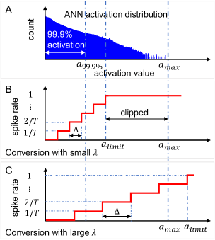
, where is the maximum value of activations mapped to the maximum spike rate (), and is the quantization resolution. In ANN-to-SNN conversion, the activations of ANNs are quantized and then, the quantized activations are mapped to their corresponding spike rate, where some quantization error is unavoidable. To reduce the quantization error due to ANN-to-SNN conversion, we need to make smaller , which can be obtained by increasing the latency, , or decreasing . This is the reason why after ANN-to-SNN conversion, latency and accuracy have trade-off relation. In the ANN-to-SNN conversion with data-normalization, is proportional to , where smaller with the fixed tends to reduce . This results in the reduction of the quantization error. However, from a certain point, is lower than and then, we have the conversion loss due to the clipping of activations, shown in Fig. 1.B, degrading the accuracy of converted SNNs as well. On the other hand, larger accompanies the increment of the quantization error, as shown in Fig. 1.C.
The work in [9] determined the norm-factor of each layer by taking the maximum value among the activation parameters of the layer. However, in order to reduce quantization error, this approach requires large latency in SNNs. The authors of [10] and [13] decreased by the following technique. In ANNs, most activations, roughly 99.0% to 99.99%, are placed in the range of of . From this observation, they decide by selecting the value of 99.9%. The authors of [11] and [12] chose based on the operation of SNN. They sequentially run SNN layers and take the maximum weighted spike output for , then scaled with the factor of . Although the smaller due to these techniques reduces quantization error, the conversion loss due to clipping error still causes significant accuracy degradation in SNNs.
In this work, we propose a novel technique to alleviate the trade off between quantization and clipping errors, where we decrease as small as possible while maintaining the accuracy of ANNs accuracy. Such an approach provides both low latency and high accuracy in SNNs, discussed in Section III-B.
III-B Trainable Clipping Layer
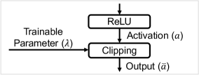
To decide the norm-factor of a certain layer, instead of analyzing activations of the corresponding ANN layer, we add a clipping layer after the ReLUs of the ANN layer, shown in Fig. 2. The forward function of the clipping layer is described in (9). Please, note that the clipping layer has a trainable parameter, , which becomes the norm-factor for the data-normalization. When backward computations of ANNs are processed, the gradients of are formulated as (10). is trained based on the learning rule of (11), where L2-regularization is used to optimize .
| (9) |
| (10) |
| (11) |
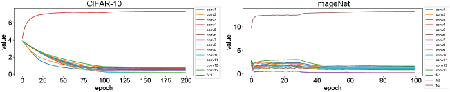
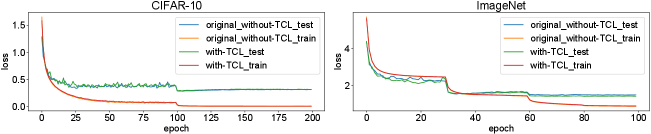
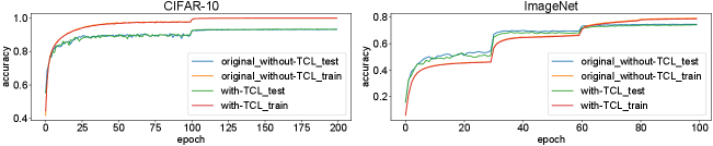
, where is the learning rate, is the L2-regularization coefficient, and is the ANN loss. We visualize the training process of norm-factors, shown in Fig. 3. The results are obtained from the training of VGG-16 for two datasets, CIFAR-10 and ImageNet. In (11), the L2-regularization term () tends to decrease , the norm-fact of the current layer, as already mentioned. From a certain point, the decrement of causes training loss. Under this situation, the optimization term () increases to complement the training loss. After some epochs, starts to be stabilized to the optimal value with respect to the training loss. Fig. 4 shows training and test losses of each training epoch. We compare training and test losses of the original ANN training, where our TCL is not used, to those of our TCL-based ANN training. Further, we observe validation accuracies of each epoch, shown in Fig. 5, clearly demonstrating that our TCL hardly affect the training results of VGG-16.
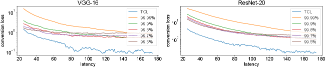
To further prove the efficacy of our TCL, we investigate how our TCL affect the loss of ANN-to-SNN conversion by comparing the conversion loss due to our TCL to those due to various norm-factors, 99.99%, 99.9%, 99.8%, 99.7%, and 99.5%, shown in Fig. 6. The conversion loss due to our TCL is significantly lower compared to the others, well showing that our TCL improves the accuracy of SNNs compared to [10, 11, 12, 13].
IV Experimental results
We implemented our TCL on a Pytorch framework [16]. We trained ANNs by using a stochastic gradient descent algorithm. We ensured that the total training epochs are 200 for CIFAR-10, and 100 for ImageNet. We initialize learning rates to besides VGG-16 and CNET with CIFAR-10, whose initial learning rates are . We scaled the learning rates by at the training epochs of [100, 150] for CIFAR-10 and [30, 60, 80] for ImageNet. The initial value of is set to for all networks with both CIFAR-10 and ImageNet datasets.
IV-A The Effect of a L2-regularization Coefficient
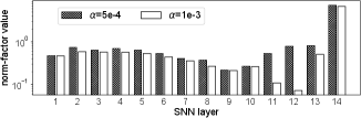
In our TCL, the L2-regularization coefficient of (11), , affects the accuracy of SNNs with the following two styles. Firstly, as shown in Fig. 7, larger tends to provide smaller norm-factors, resulting in enhanced SNN accuracy under very small latency constraints below 50 cycles. Secondly, in our TCL-based training the accuracy of ANNs shows the trend to become lower as increases, potentially lowering corresponding SNN accuracies with moderate latency conditions above 200 cycles. The above two trends clearly appear in our experiment results, shown in Table I. Since the above two trends oppositely influence the accuracy of SNNs, we need to find the optimal , the largest value not to affect the accuracy of ANNs. However, the algorithm to find the optimal values of hyper-parameters such as the L2-regularization coefficient is not well-established in previous researches yet, not explored in this work. From some trial and errors, we properly selected the values of in this work.
| Network | ANN accuracy | SNN accuracy | ||||
| T=20 | T=25 | T=30 | T=35 | |||
| CIFAR-10 | ||||||
| VGG-16 | 5e-4 | 93.49 | 88.33 | 92.02 | 92.48 | 92.66 |
| 1e-3 | 93.25 | 92.60 | 93.03 | 93.07 | 93.12 | |
| ResNet-20 | 1e-4 | 92.20 | 85.55 | 87.88 | 89.30 | 89.88 |
| 5e-4 | 91.58 | 89.63 | 90.50 | 90.98 | 91.22 | |
| MobileNet | 1e-4 | 91.68 | - | - | 10.02 | 20.53 |
| 5e-4 | 91.17 | - | - | 64.29 | 87.50 | |
| ImageNet | ||||||
| VGG-16 | 1e-4 | 73.91 | - | 57.42 | 64.20 | 67.59 |
| 1e-3 | 73.22 | - | 65.72 | 69.36 | 70.75 | |
IV-B Experiment results and discussion
| Model | Architecture | ANN accuracy | ANN accuracy | SNN | Latency | Conversion |
| (without TCL) | (with TCL) | accuracy | loss | |||
| CIFAR-10 | ||||||
| Cao et al. (2015)[8] | CNN (3Conv, 2Linear) | 79.12 | - | 77.43 | 400 | 1.69 |
| Rueckaur et al. (2017) [10] | CNN (4Conv, 2Linear) | 91.91 | - | 90.85 | 400 | 1.06 |
| Sengupta et al. (2019) [11] | VGG-16 | 91.70 | - | 91.55 | 2500 | 0.15 |
| ResNet-20 | 89.10 | - | 87.46 | 2500 | 1.64 | |
| Han et al. (2020) [12] | VGG-16 | 93.63 | - | 93.51 | 1024 | 0.12 |
| ResNet-20 | 91.47 | - | 91.36 | 2048 | 0.11 | |
| Rathi et al. (2020) [14] | VGG-16 | 92.81 | - | 92.02 | 200 | 0.79 |
| ResNet-20 | 93.15 | - | 92.22 | 250 | 0.93 | |
| Rathi & Roy (2020) [15] | VGG-16 | 93.72 | - | 92.64 | 20 | 1.08 |
| ResNet-20 | 92.79 | - | 92.14 | 25 | 0.65 | |
| Ours | CNET (4Conv, 2Linear) | 89.96 | 90.05 () | 90.04 | 100 | 0.01 |
| VGG-16 | 93.28 | 93.49 () | 93.33 | 100 | 0.16 | |
| 93.25 () | 92.60 | 20 | 0.65 | |||
| ResNet-20 | 92.26 | 92.20 () | 91.78 | 100 | 0.42 | |
| 92.06 | 150 | 0.14 | ||||
| 91.58 () | 90.50 | 25 | 1.08 | |||
| MobileNet | 91.81 | 91.68 () | 91.26 | 150 | 0.42 | |
| 91.48 | 200 | 0.20 | ||||
| 91.17 () | 87.50 | 35 | 3.67 | |||
| ImageNet | ||||||
| Rueckaur et al. (2017) [10] | VGG-16 | 63.89 | - | 49.61 | 400 | 14.28 |
| Inception-V3 | 76.12 | - | 74.60 | 550 | 1.52 | |
| Sengupta et al. (2019) [11] | VGG-16 | 70.52 | - | 69.96 | 2500 | 0.56 |
| ResNet-34 | 70.69 | - | 65.47 | 2500 | 5.22 | |
| Lu & Sengupta (2020) [13] | VGG-15 | 69.05 | - | 66.56 | 64 | 2.49 |
| Han et al. (2020) [12] | VGG-16 | 73.49 | - | 73.09 | 4096 | 0.40 |
| ResNet-34 | 70.64 | - | 69.89 | 4096 | 0.75 | |
| Rathi et al. (2020) [14] | VGG-16 | 69.35 | - | 65.19 | 250 | 4.16 |
| ResNet-34 | 70.02 | - | 61.48 | 250 | 8.54 | |
| Rathi & Roy (2020) [15] | VGG-16 | 70.08 | - | 66.52 | 25 | 3.56 |
| Ours | VGG-16 | 73.85 | 73.91 () | 73.79 | 150 | 0.12 |
| 73.87 | 250 | 0.04 | ||||
| 73.22 () | 70.75 | 35 | 2.47 | |||
| ResNet-34 | 70.87 | 70.85 () | 70.37 | 250 | 0.48 | |
| 70.66 | 300 | 0.19 | ||||
| ResNet-50 | 75.42 | 75.33 () | 74.59 | 350 | 0.74 | |
| MobileNet | 70.54 | 66.82 () | 66.57 | 350 | 0.25 | |
Our experiment results are summarized and compared to those of state-of-the-arts (SOTAs) related to ANN-to-SNN conversion in Table II. For CIFAR-10, [8], [10], [11], and [12] achieve good SNN accuracies after the ANN-to-SNN conversion. However, large latencies are required for those techniques. Although the authors of [14, 15] alleviate the large latency problem by using their proposed hybrid training technique, where they reduce their latency to the cycles of 20250, the accuracy loss due to the ANN-to-SNN conversion is still significant, larger than . Our TCL technique makes the following two significant accomplishments compared to SOTAs.
-
•
In spite of limiting the range of activations, our TCL technique hardly affect the accuray of ANNs.
-
•
After ANN-to-SNN conversion, SNNs show accuracies comparable to their ANN counterparts with moderate latency conditions.
In the dataset of CIFAR-10, with the latency of 100150 cycles, the accuracy loss due to the ANN-to-SNN conversion is almost negligible, less than . The results of ImageNet further validate our contributions, where the training results of ANNs based on our TCL are almost same to their original accuracies. In addition, with the moderate latency of 250 cycles, we obtain good SNN accuracies, almost comparable to their ANN counterparts.
For very low latencies below 50 cycles , we train ANNs with a little larger . The results show almost comparable accuracy to the hybrid training of [15], optimized for small latency constraints. Unlike [15], where the direct SNN training phase in addition to the training one of ANN requires very large computational overhead, our TCL delivers good SNN accuracy with the only ANN training phase, our significant contribution as well.
V Conclusion
Many researches have shown that ANN-to-SNN conversion can become a realistic alternative to the direction training of SNNs. However, SNNs suffer from large latency, more problematic for large size dataset such as ImageNet, limiting the possibility of SNNs. In this work, we present a trainable clipping layer technique based on the ANN-to-SNN conversion, namely TCL, alleviating the trade-off relation between accuracy and latency of SNNs. Our experiment results shows that our TCL-based SNNs obtain almost comparable accuracy to their ANN counterpart for ImageNet even with the small latency of 250 clock cycles, well validating the efficacy of our TCL technique.
References
- [1] Dongsung Huh and Terrence J. Sejnowski. Gradient descent for spiking neural networks. In NIPS, page 1440–1450. Curran Associates Inc., 2018.
- [2] Chankyu Lee, Syed Shakib Sarwar, and Kaushik Roy. Enabling spike-based backpropagation in state-of-the-art deep neural network architectures. CoRR, abs/1903.06379, 2019.
- [3] Chankyu Lee, Syed Shakib Sarwar, Priyadarshini Panda, Gopalakrishnan Srinivasan, and Kaushik Roy. Enabling spike-based backpropagation for training deep neural network architectures. Frontiers in Neuroscience, 14:119, 2020.
- [4] Yingyezhe Jin, Wenrui Zhang, and Peng Li. Hybrid macro/micro level backpropagation for training deep spiking neural networks. In S. Bengio, H. Wallach, H. Larochelle, K. Grauman, N. Cesa-Bianchi, and R. Garnett, editors, NIPS, volume 31. Curran Associates, Inc., 2018.
- [5] Yujie Wu, Lei Deng, Guoqi Li, Jun Zhu, and Luping Shi. Spatio-temporal backpropagation for training high-performance spiking neural networks. Frontiers in Neuroscience, 12:331, 2018.
- [6] Guillaume Bellec, Darjan Salaj, Anand Subramoney, Robert Legenstein, and Wolfgang Maass. Long short-term memory and learning-to-learn in networks of spiking neurons. In NIPS, page 795–805. Curran Associates Inc., 2018.
- [7] Emre Ozgur Neftci, Hesham Mostafa, and Friedemann Zenke. Surrogate gradient learning in spiking neural networks. CoRR, abs/1901.09948, 2019.
- [8] Yongqiang Cao, Yang Chen, and Deepak Khosla. Spiking deep convolutional neural networks for energy-efficient object recognition. Int. J. Comput. Vision, 113(1):54–66, 2015.
- [9] Peter U. Diehl, Daniel Neil, Jonathan Binas, Matthew Cook, Shih-Chii Liu, and Michael Pfeiffer. Fast-classifying, high-accuracy spiking deep networks through weight and threshold balancing. In IJCNN, pages 1–8, 2015.
- [10] Bodo Rueckauer, Iulia-Alexandra Lungu, Yuhuang Hu, Michael Pfeiffer, and Shih-Chii Liu. Conversion of continuous-valued deep networks to efficient event-driven networks for image classification. Frontiers in Neuroscience, 11:682, 2017.
- [11] Abhronil Sengupta, Yuting Ye, Robert Wang, Chiao Liu, and Kaushik Roy. Going deeper in spiking neural networks: Vgg and residual architectures. Frontiers in Neuroscience, 13:95, 2019.
- [12] Bing Han, G. Srinivasan, and K. Roy. Rmp-snn: Residual membrane potential neuron for enabling deeper high-accuracy and low-latency spiking neural network. CVPR, pages 13555–13564, 2020.
- [13] Sen Lu and Abhronil Sengupta. Exploring the connection between binary and spiking neural networks. arXiv preprint arXiv:2002.10064, 2020.
- [14] Nitin Rathi, Gopalakrishnan Srinivasan, Priyadarshini Panda, and Kaushik Roy. Enabling deep spiking neural networks with hybrid conversion and spike timing dependent backpropagation. In ICLR, 2020.
- [15] Nitin Rathi and Kaushik Roy. Diet-snn: Direct input encoding with leakage and threshold optimization in deep spiking neural networks, 2020.
- [16] Adam Paszke, Sam Gross, Francisco Massa, Adam Lerer, James Bradbury, Gregory Chanan, Trevor Killeen, Zeming Lin, Natalia Gimelshein, Luca Antiga, Alban Desmaison, Andreas Kopf, Edward Yang, Zachary DeVito, Martin Raison, Alykhan Tejani, Sasank Chilamkurthy, Benoit Steiner, Lu Fang, Junjie Bai, and Soumith Chintala. Pytorch: An imperative style, high-performance deep learning library. In NIPS, pages 8024–8035. Curran Associates, Inc., 2019.