Technical Report # KU-EC-08-5:
QR-Adjustment for Clustering Tests Based on Nearest Neighbor Contingency Tables

NNCTs are constructed using the NN frequencies of classes. I describe the construction of NNCTs for two classes; extension to multi-class case is straightforward. Consider two classes with labels $\{1,2\}$. Let $N_{i}$ be the number of points from class $i$ for $i\in\{1,2\}$ and $n$ be the total sample size, so $n=N_{1}+N_{2}$. If I record the class of each point and the class of its NN, the NN relationships fall into four distinct categories: $(1,1),\,(1,2);\,(2,1),\,(2,2)$ where in cell $(i,j)$, class $i$ is the base class, while class $j$ is the class of its NN. That is, the $n$ points constitute $n$ (base, NN) pairs. Then each pair can be categorized with respect to the base label (row categories) and NN label (column categories). Denoting $N_{ij}$ as the frequency of cell $(i,j)$ for $i,j\in\{1,2\}$, I obtain the NNCT in Table 1 where $C_{j}$ is the sum of column $j$; i.e., number of times class $j$ points serve as NNs for $j\in\{1,2\}$. Furthermore, $N_{ij}$ is the cell count for cell $(i,j)$ that is the sum of all (base, NN) pairs each of which has label $(i,j)$. Note also that $n=\sum_{i,j}N_{ij}$; $n_{i}=\sum_{j=1}^{2}\,N_{ij}$; and $C_{j}=\sum_{i=1}^{2}\,N_{ij}$. By construction, if $N_{ij}$ is larger (smaller) than expected, then class $j$ serves as NN more (less) to class $i$ than expected, which implies (lack of) segregation if $i=j$ and (lack of) association of class $j$ with class $i$ if $i\not=j$. Hence, column sums, cell counts are random, while row sums and the overall sum are fixed quantities in a NNCT.

Observe that, under segregation, the diagonal entries, $N_{ii}$ for $i=1,2$, tend to be larger than expected; under association, the off-diagonals tend to be larger than expected. The general alternative is that some cell counts are different than expected under CSR independence or RL.

In the two-class case, Pielou, (1961) used Pearson’s $\chi^{2}$-test of independence to detect any deviation from CSR independence or RL. But, under CSR independence or RL, this test is liberal, i.e., has larger size than the nominal level (Ceyhan, (2006)), hence not considered in this article. Dixon, (1994) proposed a series of tests for segregation based on NNCTs. He first devised four cell-specific tests in the two-class case, and then combined them to form an overall test. For his tests, the probability of an individual from class $j$ serving as a NN of an individual from class $i$ depends only on the class sizes (i.e., row sums), but not the total number of times class $j$ serves as NNs (i.e., column sums).

The level of segregation is estimated by comparing the observed cell counts to the expected cell counts under RL of points that are fixed. Dixon demonstrates that under RL, one can write down the cell frequencies as Moran join count statistics (Moran, (1948)). He then derives the means, variances, and covariances of the cell counts (frequencies) in a NNCT (Dixon, (1994, 2002)).

The null hypothesis under RL is given by

Observe that the expected cell counts depend only on the size of each class (i.e., row sums), but not on column sums.

The cell-specific test statistics suggested by Dixon are given by

where

with $p_{xx}$, $p_{xxx}$, and $p_{xxxx}$ are the probabilities that a randomly picked pair, triplet, or quartet of points, respectively, are the indicated classes and are given by

Furthermore, $Q$ is the number of points with shared NNs, which occur when two or more points share a NN and $R$ is twice the number of reflexive pairs. Then $Q=2\,(Q_{2}+3\,Q_{3}+6\,Q_{4}+10\,Q_{5}+15\,Q_{6})$ where $Q_{k}$ is the number of points that serve as a NN to other points $k$ times. One-sided and two-sided tests are possible for each cell $(i,j)$ using the asymptotic normal approximation of $Z^{D}_{ij}$ given in Equation (2) (Dixon, (1994)). The test in Equation (2) is the same as Dixon’s $Z_{AA}$ when $i=j=1$; same as $Z_{BB}$ when $i=j=2$ (Dixon, (1994)). Note also that in Equation (2) four different tests are defined as there are four cells and each is testing the deviation from the null case in the respective cell. These four tests are combined and used in defining an overall test of segregation in Section 2.4.

Under CSR independence, the null hypothesis, the test statistics, and the variances are as in the RL case for the cell-specific tests, except for the fact that the variances are conditional on $Q$ and $R$.

Note the difference in status of the variables $Q$ and $R$ under CSR independence and RL models. Under RL, $Q$ and $R$ are fixed quantities; while under CSR independence, they are random. The quantities given in Equations (1), (3), and all the quantities depending on these expectations also depend on $Q$ and $R$. Hence these expressions are appropriate under the RL pattern. Under CSR independence pattern they are conditional variances and covariances obtained by using the observed values of $Q$ and $R$. The unconditional variances and covariances can be obtained by replacing $Q$ and $R$ with their expectations.

Unfortunately, given the difficulty of calculating the expectations of $Q$ and $R$ under CSR independence, Ceyhan, (2007) employed the conditional variances and covariances (i.e., the variances and covariances for which observed $Q$ and $R$ values are used) even when assessing their behavior under CSR independence pattern. Alternatively, I can estimate the values of $Q$ and $R$ empirically as follows. I generate $n\in\{10,20,30,40,50,100,500,1000\}$ points that are iid (independently and identically distributed) from $\mathcal{U}((0,1)\times(0,1))$, the uniform distribution on the unit square. I repeat this procedure $N_{mc}=1000000$ times. At each Monte Carlo replication, I calculate $Q$ and $R$ values, and record the ratios $Q/n$ and $R/n$. I plot these ratios in Figure 1 as a function of sample size $n$. Observe that the ratios seem to converge as $n$ increases. For homogeneous planar Poisson pattern, I have $\mathbf{E}[Q/n]\approx.6327860$ and $\mathbf{E}[R/n]\approx 0.6211200$. Hence, I replace $Q$ and $R$ by $0.63\,n$ and $0.62\,n$, respectively, to obtain the QR-adjusted variances and covariances.

Dixon’s overall test of segregation tests the hypothesis that expected cell counts in the NNCT are as in Equation (1). In the two-class case, he calculates $Z_{ii}=(N_{ii}-\mathbf{E}[N_{ii}])\big{/}\sqrt{\mathbf{Var}[N_{ii}]}$ for both $i\in\{1,2\}$ and combines these test statistics into a statistic that is asymptotically distributed as $\chi^{2}_{2}$ under RL (Dixon, (1994)). The suggested test statistic is given by

where $\mathbf{E}[N_{ii}]$ are as in Equation (1), $\mathbf{Var}[N_{ii}]$ are as in Equation (3), and

Dixon’s $C$ statistic given in Equation (5) can also be written as

where $r=\mathbf{Cov}[N_{11},N_{22}]\Big{/}\sqrt{\mathbf{Var}[N_{11}]\mathbf{Var}[N_{22}]}$ (Dixon, (1994)).

Under CSR independence, the expected values, variances and covariances are as in the RL case. However, the variance and covariance terms include $Q$ and $R$ which are random under CSR independence and fixed under RL. Hence Dixon’s test statistic $C$ asymptotically has a $\chi^{2}_{1}$-distribution under CSR independence conditional on $Q$ and $R$. Replacing $Q$ and $R$ by their empirical estimates given in Section 2.3, I obtain the QR-adjusted version of Dixon’s test which is denoted by $C_{qr}$.

Ceyhan, (2007) proposed tests based on the correct sampling distribution of the cell counts in a NNCT under CSR independence or RL. In defining the new segregation or clustering tests, I follow a track similar to that of Dixon’s (Dixon, (1994)) where he defines a cell-specific test statistic for each cell and then combines these four tests into an overall test.

For cell $(i,j)$, let

Furthermore, let $\mathbf{N_{I}}$ be the vector of $N^{I}_{ij}$ values concatenated row-wise and let $\Sigma_{I}$ be the variance-covariance matrix of $\mathbf{N_{I}}$ based on the correct sampling distribution of the cell counts. That is, $\Sigma_{I}=\left(\mathbf{Cov}\left[N^{I}_{ij},N^{I}_{kl}\right]\right)$ where

with $\mathbf{Cov}\left[N_{ij},N_{kl}\right]$ is as in Equation (3) if $(i,j)=(k,l)$ and as in Equation (6) if $(i,j)=(1,1)$ and $(k,l)=(2,2)$. Since $\Sigma_{I}$ is not invertible, I use its generalized inverse which is denoted by $\Sigma_{I}^{-}$ (Searle, (2006)). Then the first version of segregation tests suggested by Ceyhan, (2007) is

which asymptotically has a $\chi^{2}_{1}$ distribution.

Under CSR independence, the expected values, variances, and covariances related to $\mathcal{X}_{I}^{2}$ are as in the RL case, except they are not only conditional on column sums (i.e., on $C_{j}=c_{j}$), but also conditional on $Q$ and $R$. Hence $\mathcal{X}_{I}^{2}$ has asymptotically $\chi^{2}_{1}$ distribution conditional on column sums, $Q$ and $R$ under CSR independence. Replacing $Q$ and $R$ by their empirical estimates given in Section 2.3, I obtain the QR-adjusted version of this test which is denoted by $\mathcal{X}_{I,qr}^{2}$, which is still conditional on column sums.

For cell $(i,j)$, let

Furthermore, let $\mathbf{N_{II}}$ be the vector of $N^{II}_{ij}$ concatenated row-wise and let $\Sigma_{II}$ be the variance-covariance matrix of $\mathbf{N_{II}}$ based on the correct sampling distribution of the cell counts. That is, $\Sigma_{II}=\left(\mathbf{Cov}\left[N^{II}_{ij},N^{II}_{kl}\right]\right)$ where

Since $\Sigma_{II}$ is not invertible, I use its generalized inverse $\Sigma_{II}^{-}$. Then second version of the tests proposed by Ceyhan, (2007) is

which asymptotically has a $\chi^{2}_{2}$ distribution under RL. Note that $\Sigma_{II}$ can be obtained from $\Sigma$ used in Equation (5) by multiplying $\Sigma$ entry-wise with the matrix $C^{II}_{M}=\left(\frac{n}{\sqrt{n_{i}\,n_{j}\,n_{k}\,n_{l}}}\right)$. This version of the segregation test is asymptotically equivalent to Dixon’s segregation test.

Under CSR independence, the expectations, variances, and covariances related to $\mathcal{X}^{2}_{II}$ are as in the RL case, but the variances and covariances are conditional on $Q$ and $R$. Hence, the asymptotic distribution of $\mathcal{X}^{2}_{II}$ is also conditional on $Q$ and $R$. Replacing $Q$ and $R$ with their empirical estimates, I obtain the QR-adjusted version of this test which is denoted by $\mathcal{X}^{2}_{II,qr}$ and is not conditional any more.

Notice that version I is a conditional test (conditional on column sums), while version II is asymptotically equivalent to Dixon’s test, Furthermore, both Dixon’s test and version II incorporate only row sums (i.e., class sizes) in the NNCTs.

Ceyhan, (2007) suggests another test statistic which uses both the column sums (i.e., number of times a class serves as NN) and row sums and is not conditional on the column sums. Let

Let $\mathbf{N_{III}}$ be the vector of $T^{III}_{ij}$ values concatenated row-wise and let $\Sigma_{III}$ be the variance-covariance matrix of $\mathbf{N_{III}}$ based on the correct sampling distribution of the cell counts. That is, $\Sigma_{III}=\left(\mathbf{Cov}\left[T^{III}_{ij},T^{III}_{kl}\right]\right)$ where the explicit forms of $\mathbf{Cov}\left[T^{III}_{ij},T^{III}_{kl}\right]$ are provided in (Ceyhan, (2007)). Since $\Sigma_{III}$ is not invertible, I use its generalized inverse $\Sigma_{III}^{-}$. Then the proposed test statistic by (Ceyhan, (2007)) for overall segregation is the quadratic form $\mathcal{X}_{III}^{2}=\mathbf{N^{\prime}_{III}}\Sigma_{III}^{-}\mathbf{N_{III}}$ which asymptotically has a $\chi^{2}_{1}$ distribution.

Under CSR independence, the discussion related to and derivation of $\mathcal{X}^{2}_{III}$ are as in the RL case; however, the variance and covariance terms (hence the asymptotic distribution) are conditional on $Q$ and $R$. Replacing $Q$ and $R$ with their empirical estimates, I obtain the QR-adjusted version of this test which is denoted by $\mathcal{X}^{2}_{III,qr}$.

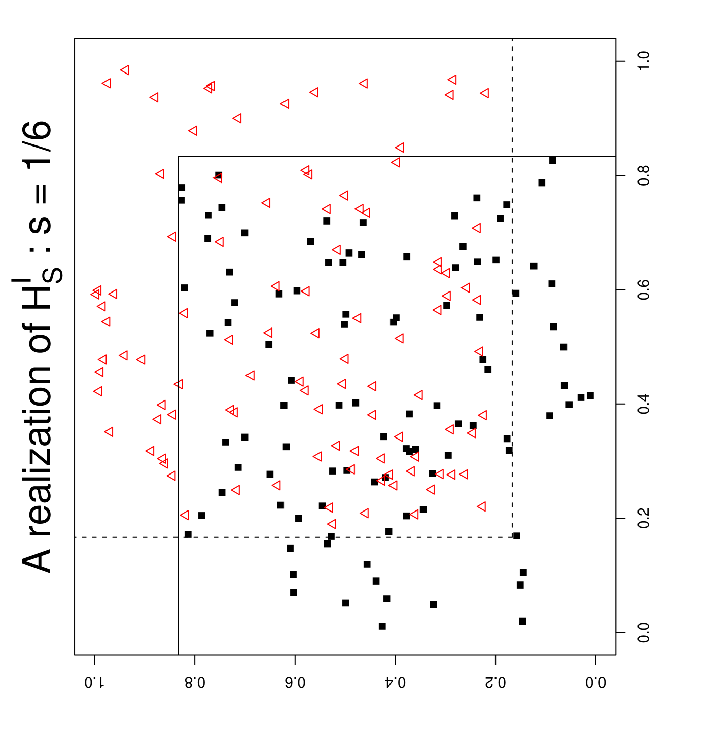
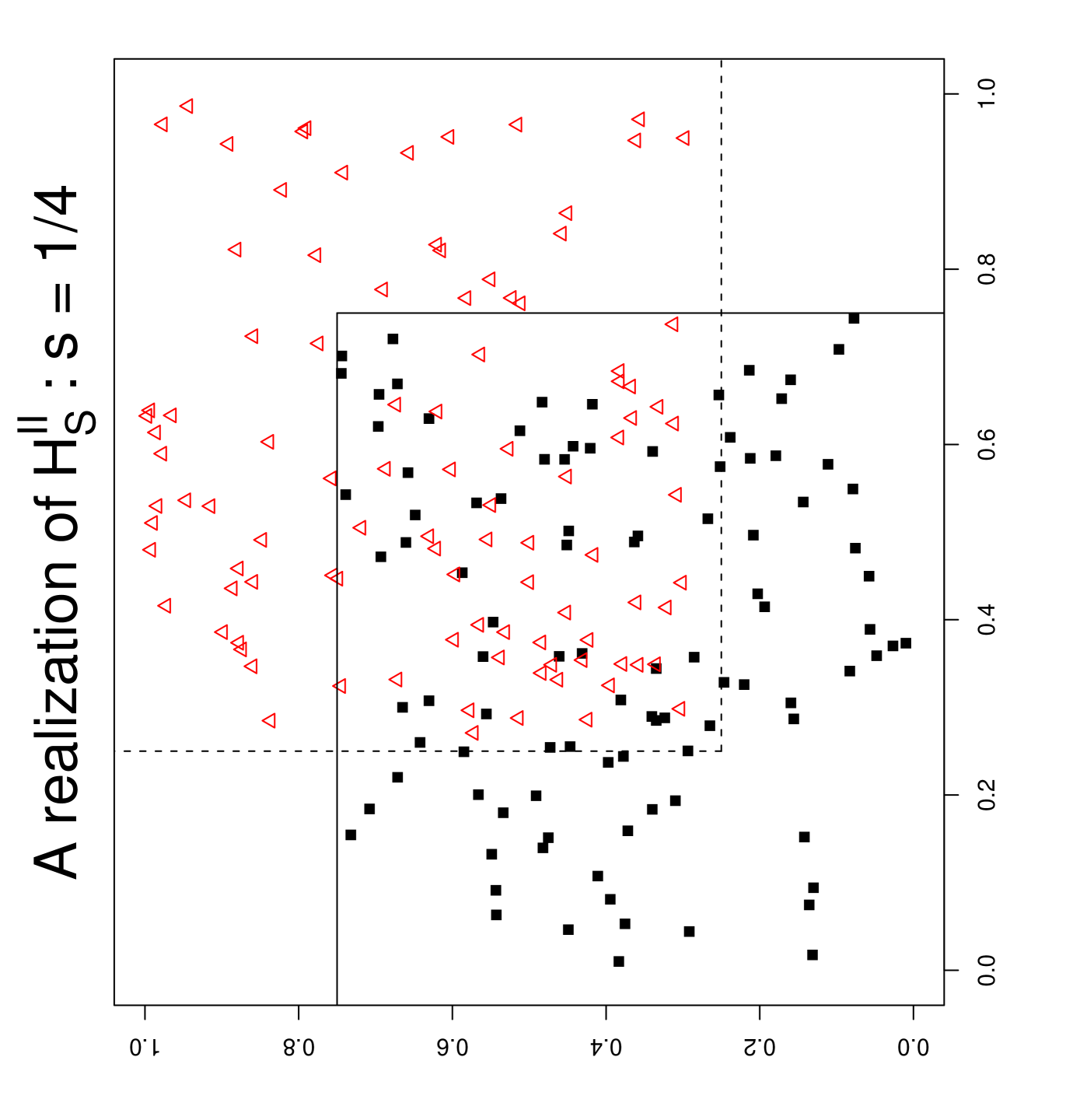
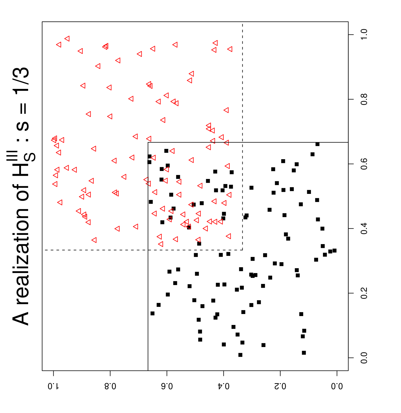
For the segregation alternatives (against the CSR pattern), three cases are considered. I generate $X_{i}\stackrel{{\scriptstyle iid}}{{\sim}}\mathcal{U}((0,1-s)\times(0,1-s))$ for $i=1,2,\ldots,n_{1}$ and $Y_{j}\stackrel{{\scriptstyle iid}}{{\sim}}\mathcal{U}((s,1)\times(s,1))$ for $j=1,2,\ldots,n_{2}$. In the pattern generated, appropriate choices of $s$ will imply $X_{i}$ and $Y_{j}$ to be more segregated than expected under CSR. That is, it will be more likely to have $(X,X)$ NN pairs than mixed NN pairs (i.e., $(X,Y)$ or $(Y,X)$ pairs). The three values of $s$ I consider constitute the three segregation alternatives:

Observe that, from $H_{S}^{I}$ to $H_{S}^{III}$ (i.e., as $s$ increases), the segregation gets stronger in the sense that $X$ and $Y$ points tend to form one-class clumps or clusters. By construction, the points are uniformly generated, hence exhibit homogeneity with respect to their supports for each class, but with respect to the unit square these alternative patterns are examples of departures from first-order homogeneity which implies segregation of the classes $X$ and $Y$. The simulated segregation patterns are symmetric in the sense that, $X$ and $Y$ classes are equally segregated (or clustered) from each other.

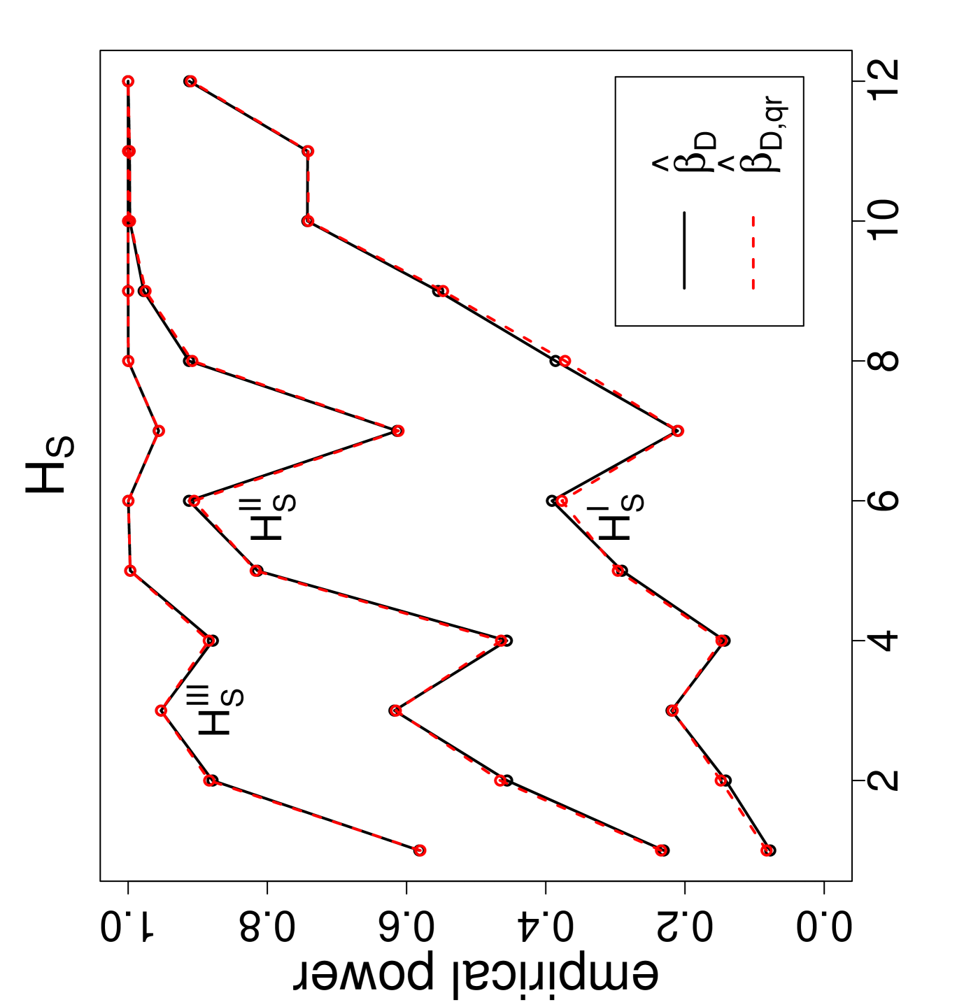
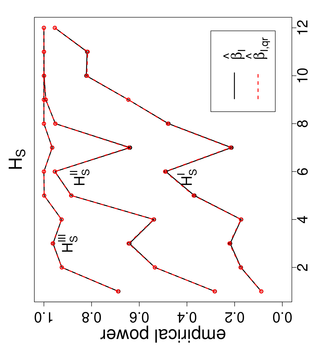
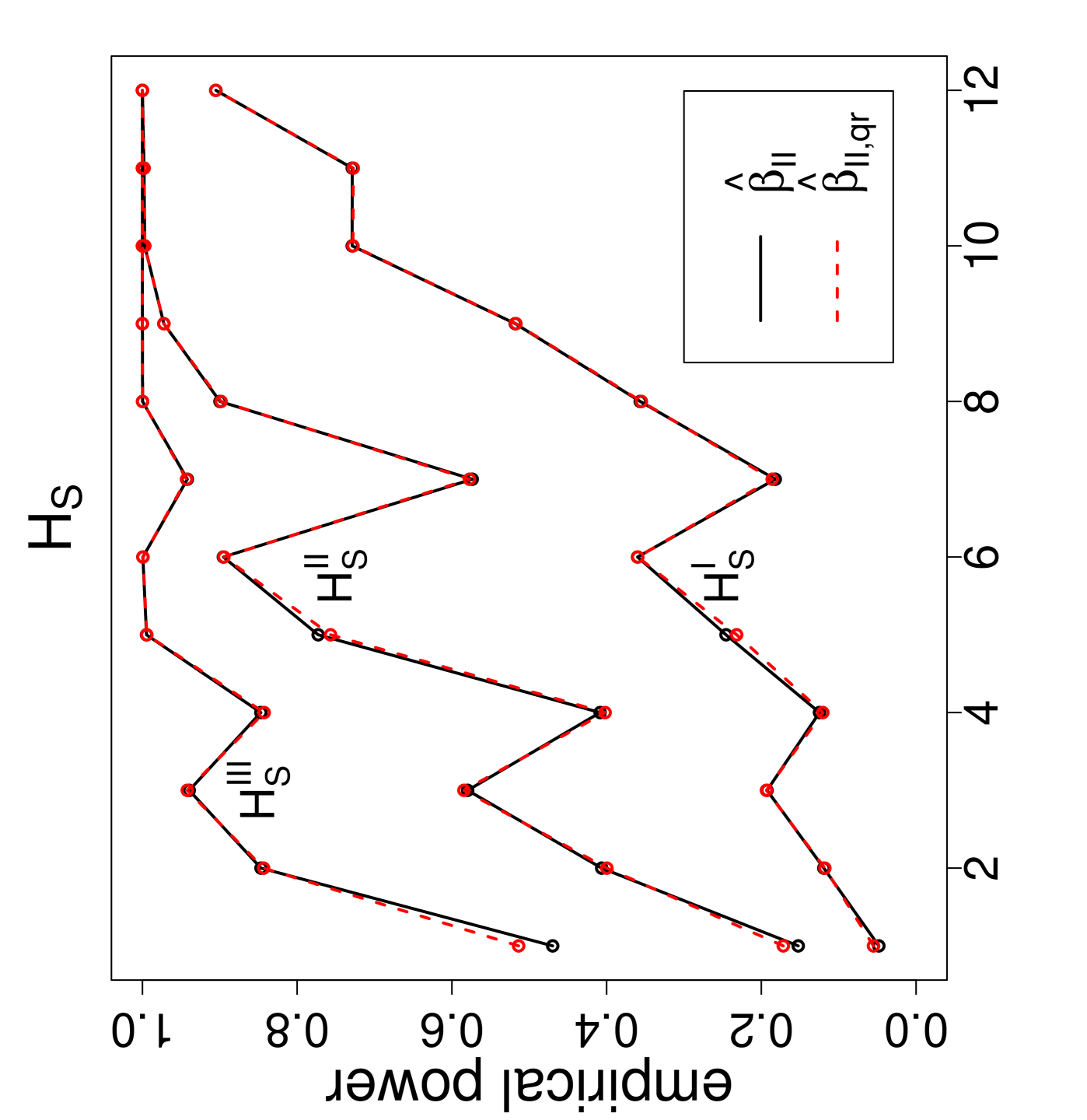
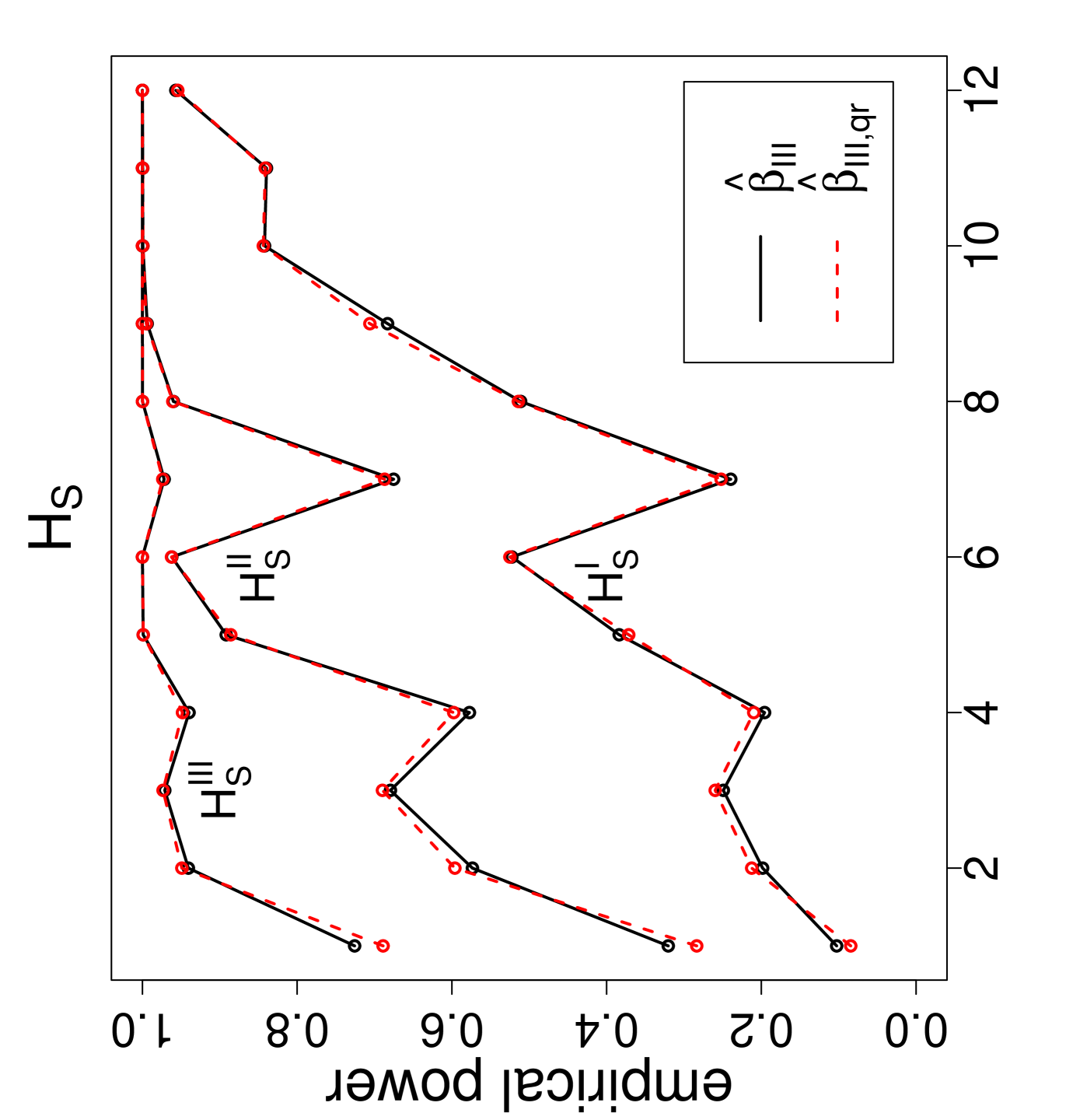
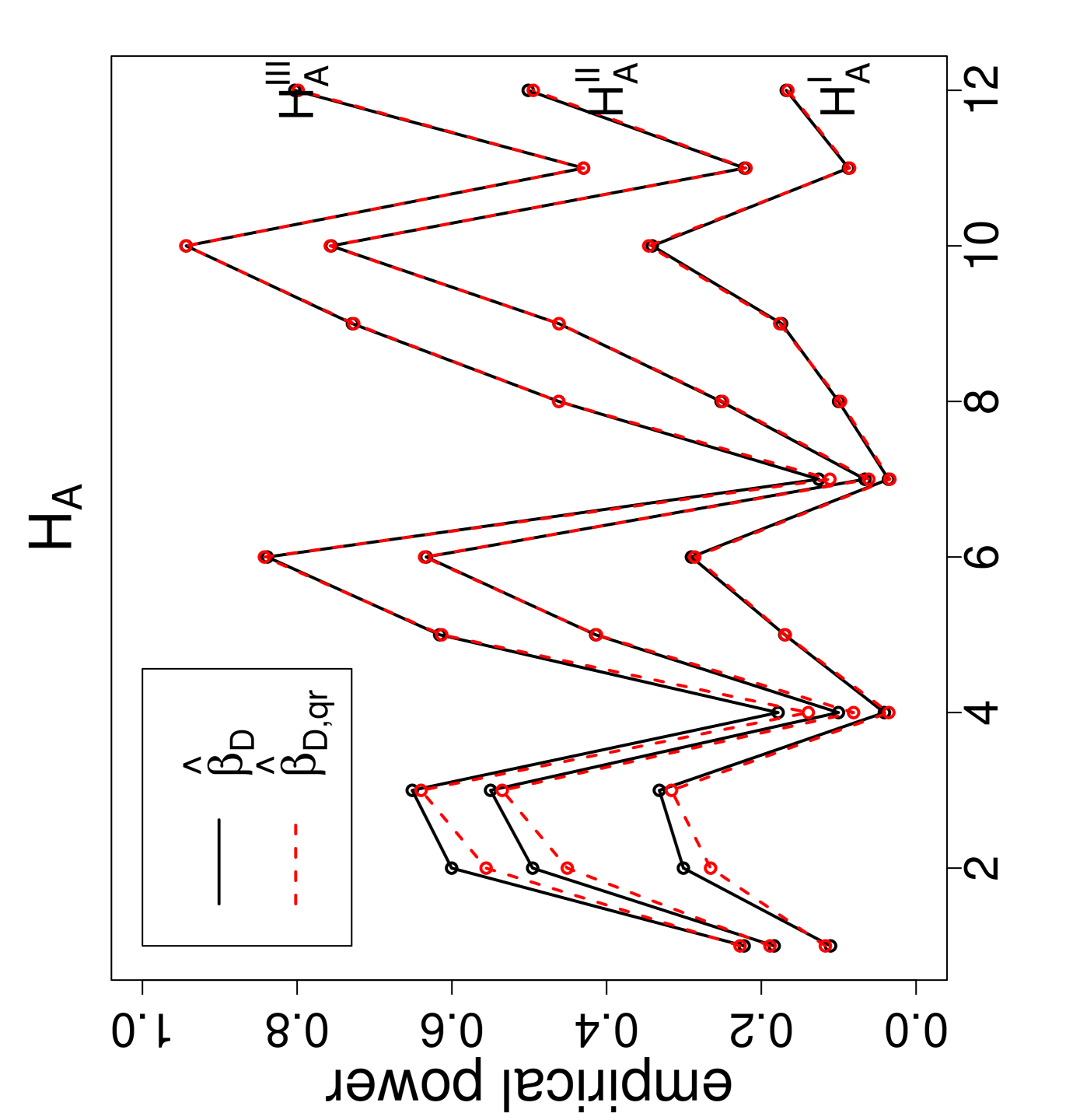
The power estimates against the sample size combinations are presented in Figure 3, where $\widehat{\beta}_{D}$ is for Dixon’s test, $\widehat{\beta}_{I}$, $\widehat{\beta}_{II}$, and $\widehat{\beta}_{III}$ are for versions I, II , and III, respectively, and the QR-adjusted versions are indicated by $qr$ in their subscripts. Observe that, as $n=(n_{1}+n_{2})$ gets larger, the power estimates get larger. For the same $n=(n_{1}+n_{2})$ values, the power estimate is larger for classes with similar sample sizes. Furthermore, as the segregation gets stronger, the power estimates get larger. The NNCT-tests have about the same power performance under these segregation alternatives. Notice also that for small samples the power estimates of the QR-adjusted versions are slightly larger but for other sample size combinations the power estimates for the QR-adjusted versions and the unadjusted versions are virtually indistinguishable.

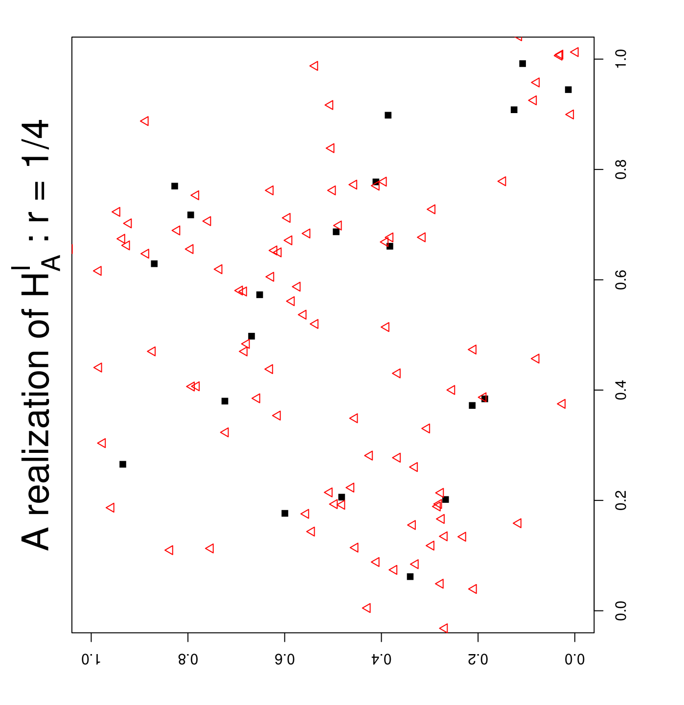
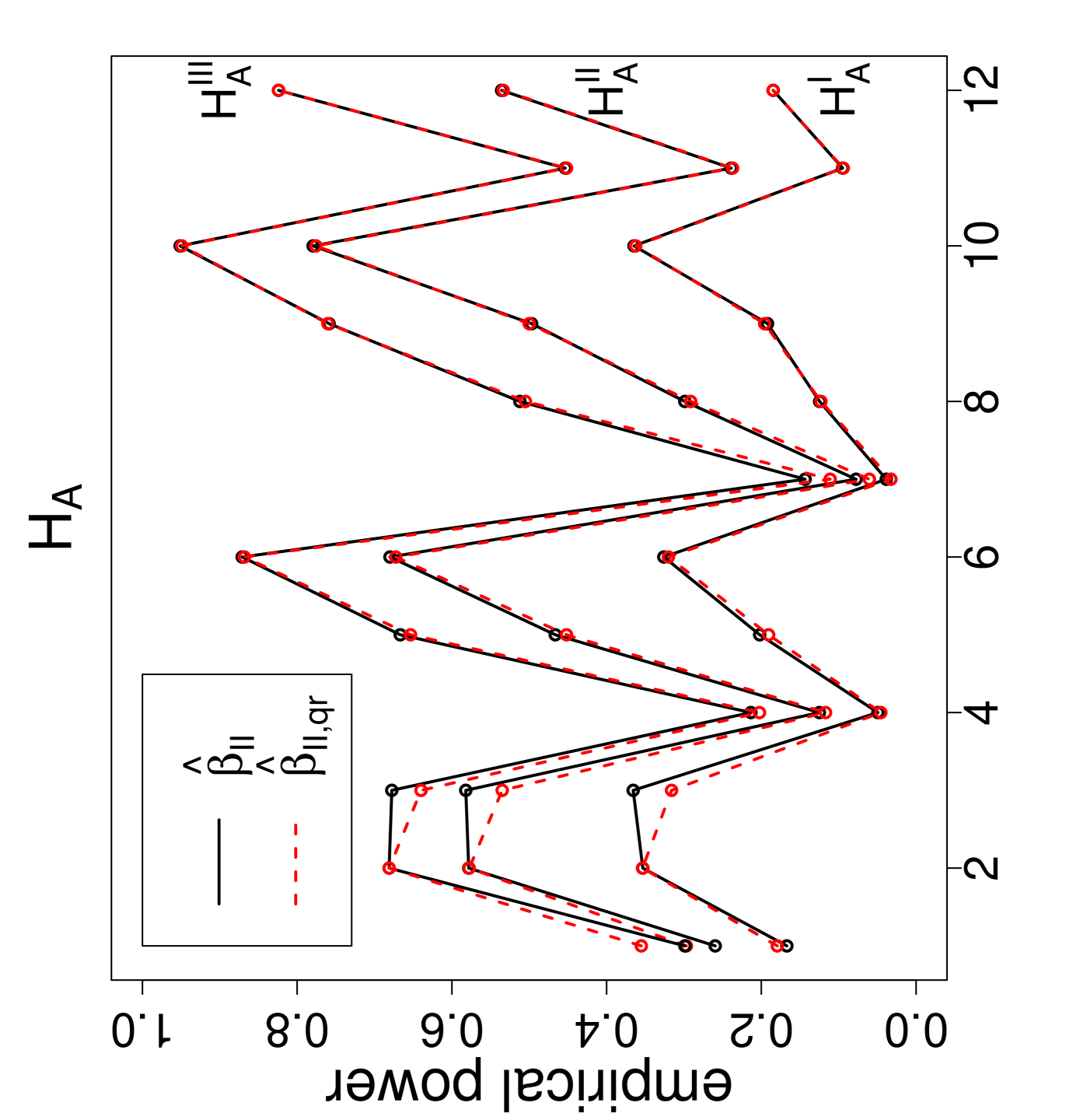
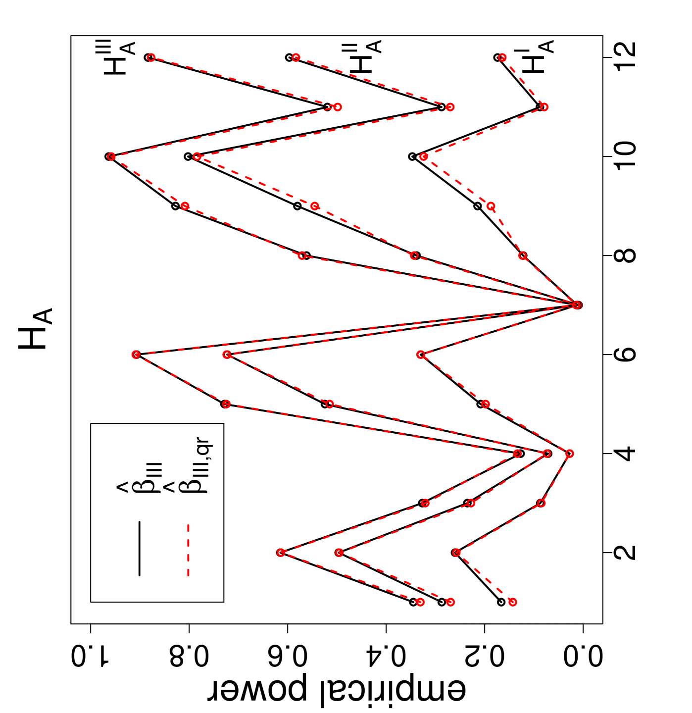
For the association alternatives (against the CSR pattern), I also consider three cases. First, I generate $X_{i}\stackrel{{\scriptstyle iid}}{{\sim}}\mathcal{U}((0,1)\times(0,1))$ for $i=1,2,\ldots,n_{1}$. Then I generate $Y_{j}$ for $j=1,2,\ldots,n_{2}$ as follows. For each $j$, I pick an $i$ randomly, then generate $Y_{j}$ as $X_{i}+R_{j}\,(\cos T_{j},\sin T_{j})^{\prime}$ where $R_{j}\stackrel{{\scriptstyle iid}}{{\sim}}\mathcal{U}(0,r)$ with $r\in(0,1)$ and $T_{j}\stackrel{{\scriptstyle iid}}{{\sim}}\mathcal{U}(0,2\,\pi)$. In the pattern generated, appropriate choices of $r$ will imply $Y_{j}$ and $X_{i}$ are more associated than expected. That is, it will be more likely to have $(X,Y)$ NN pairs than self NN pairs (i.e., $(X,X)$ or $(Y,Y)$). The three values of $r$ I consider constitute the three association alternatives:

Observe that, from $H_{A}^{I}$ to $H_{A}^{III}$ (i.e., as $r$ decreases), the association gets stronger in the sense that $X$ and $Y$ points tend to occur together more and more frequently. By construction, $X$ points are from a homogeneous Poisson process with respect to the unit square, while $Y$ points exhibit inhomogeneity in the same region. Furthermore, these alternative patterns are examples of departures from second-order homogeneity which implies association of the class $Y$ with class $X$.

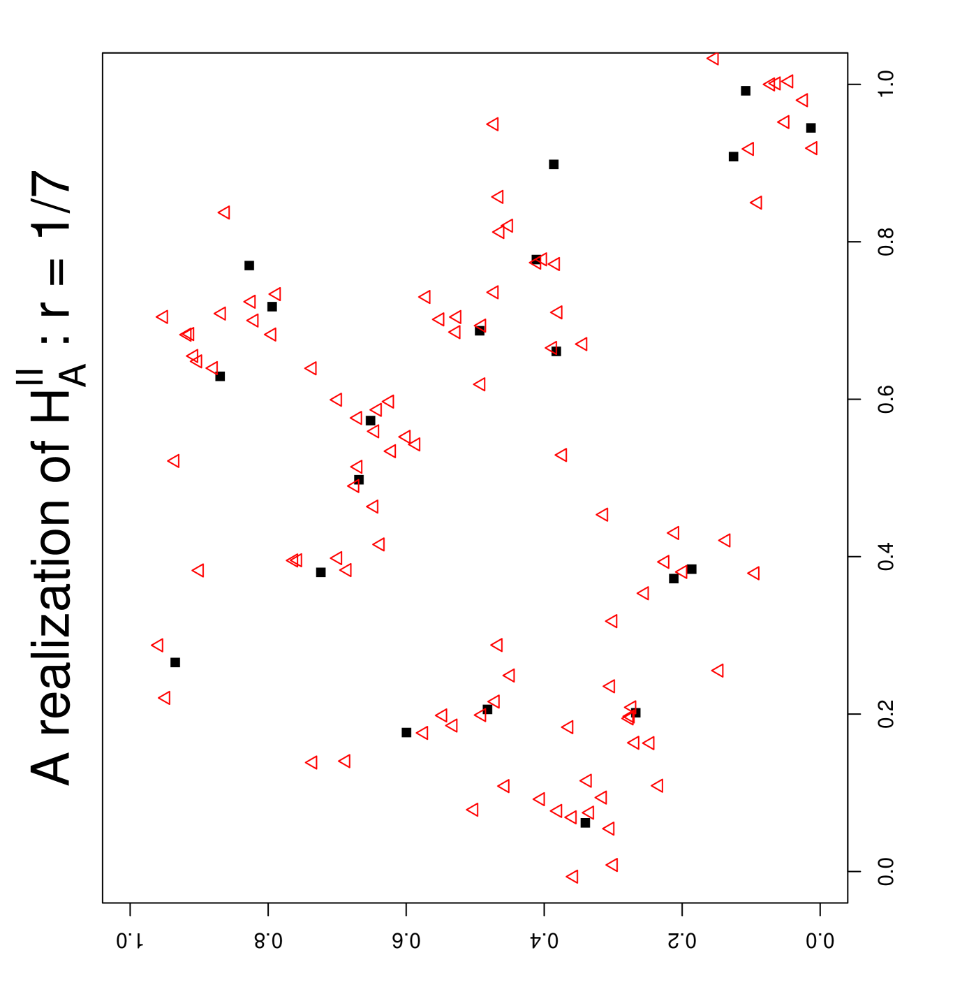
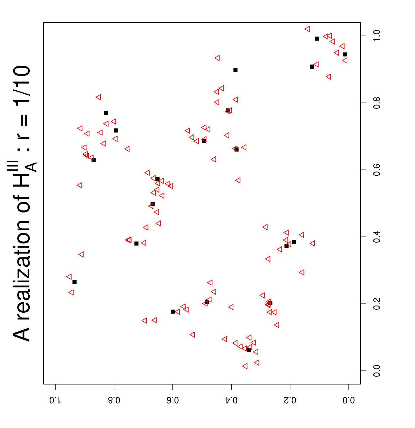
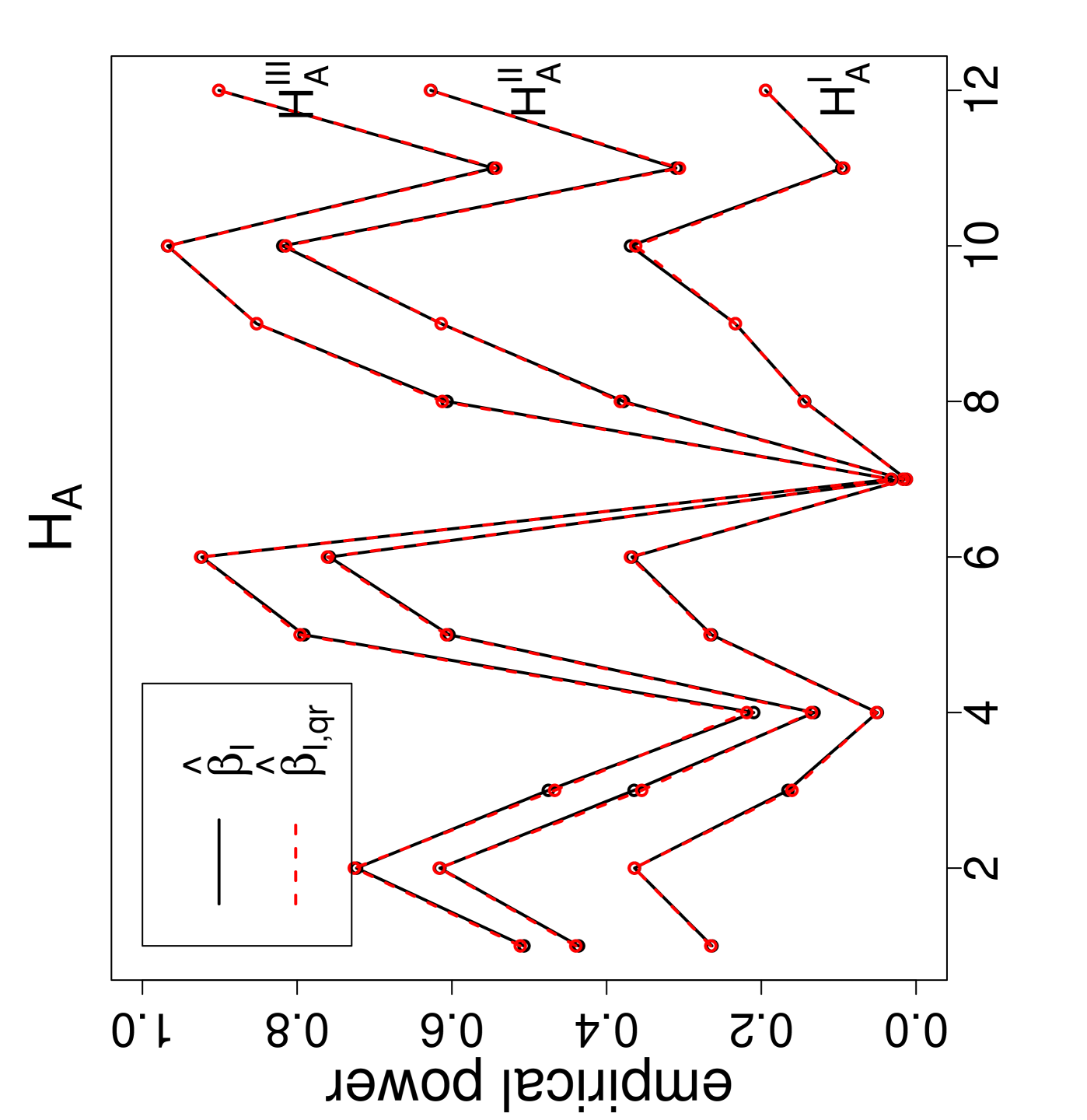
The power estimates under the association alternatives are presented in Figure 5, where labeling is as in Figure 3. Observe that, for similar sample sizes as $n=(n_{1}+n_{2})$ gets larger, the power estimates get larger at each association alternative. Furthermore, as the association gets stronger, the power estimates get larger at each sample size combination. The NNCT-tests have about the same power estimates under these association alternatives. Furthermore the QR-adjusted versions of the tests virtually have the same power estimates as the unadjusted versions; for the smaller samples QR-adjusted version has slightly lower power estimates.

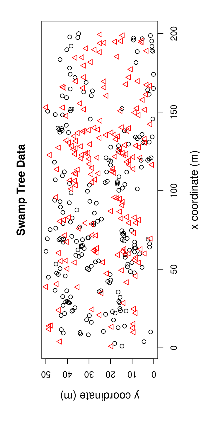
Good and Whipple, (1982) considered the spatial patterns of tree species along the Savannah River, South Carolina, U.S.A. From this data, Dixon, (2002) used a single 50m $\times$ 200m rectangular plot to illustrate his tests. All live or dead trees with 4.5 cm or more dbh (diameter at breast height) were recorded together with their species. Hence it is an example of a realization of a marked multi-variate point pattern. The plot contains 13 different tree species, four of which comprise over 90 % of the 734 tree stems. The remaining tree stems were categorized as “other trees”. The plot consists of 215 water tupelo (Nyssa aquatica), 205 black gum (Nyssa sylvatica), 156 Carolina ash (Fraxinus caroliniana), 98 bald cypress (Taxodium distichum), and 60 stems of 8 additional species (i.e., other species). I will only consider live trees from the two most frequent tree species in this data set (i.e., water tupelos and black gums). So a $2\times 2$ NNCT-analysis is conducted for this data set. If segregation among the less frequent species were important, a more detailed $5\times 5$ or a $12\times 12$ NNCT-analysis should be performed. The locations of these trees in the study region are plotted in Figure 6 and the corresponding $2\times 2$ NNCT together with percentages based on row and grand sums are provided in Table 3. For example, for water tupelo as the base species and black gum as the NN species, the cell count is 54 which is 26 % of the 211 black gums (which is 54 % of all 394 trees). Observe that the percentages and Figure 6 are suggestive of segregation for all three tree species since the observed percentages of species with themselves as the NN are much larger than the row percentages.

The locations of the tree species can be viewed a priori resulting from different processes so the more appropriate null hypothesis is the CSR independence pattern. Hence our inference will be a conditional one (see Section 2.3) if I use the observed values of $Q$ and $R$. I observe $Q=270$ and $R=236$ for this data set, and the empirical estimates for these sample sizes are $Q=249.68$ and $R=244.95$. I present the tests statistics and the associated $p$-values for NNCT-tests in Table 4. Observe that the test statistics all decrease with the QR-adjustment, however this decrease is not substantial to alter the conclusions. Based on the NNCT-tests, I find that the segregation between both species is significant, since all the tests considered yield significant $p$-values, and the diagonal cells (i.e., cells $(1,1)$ and $(2,2)$) are larger than expected.

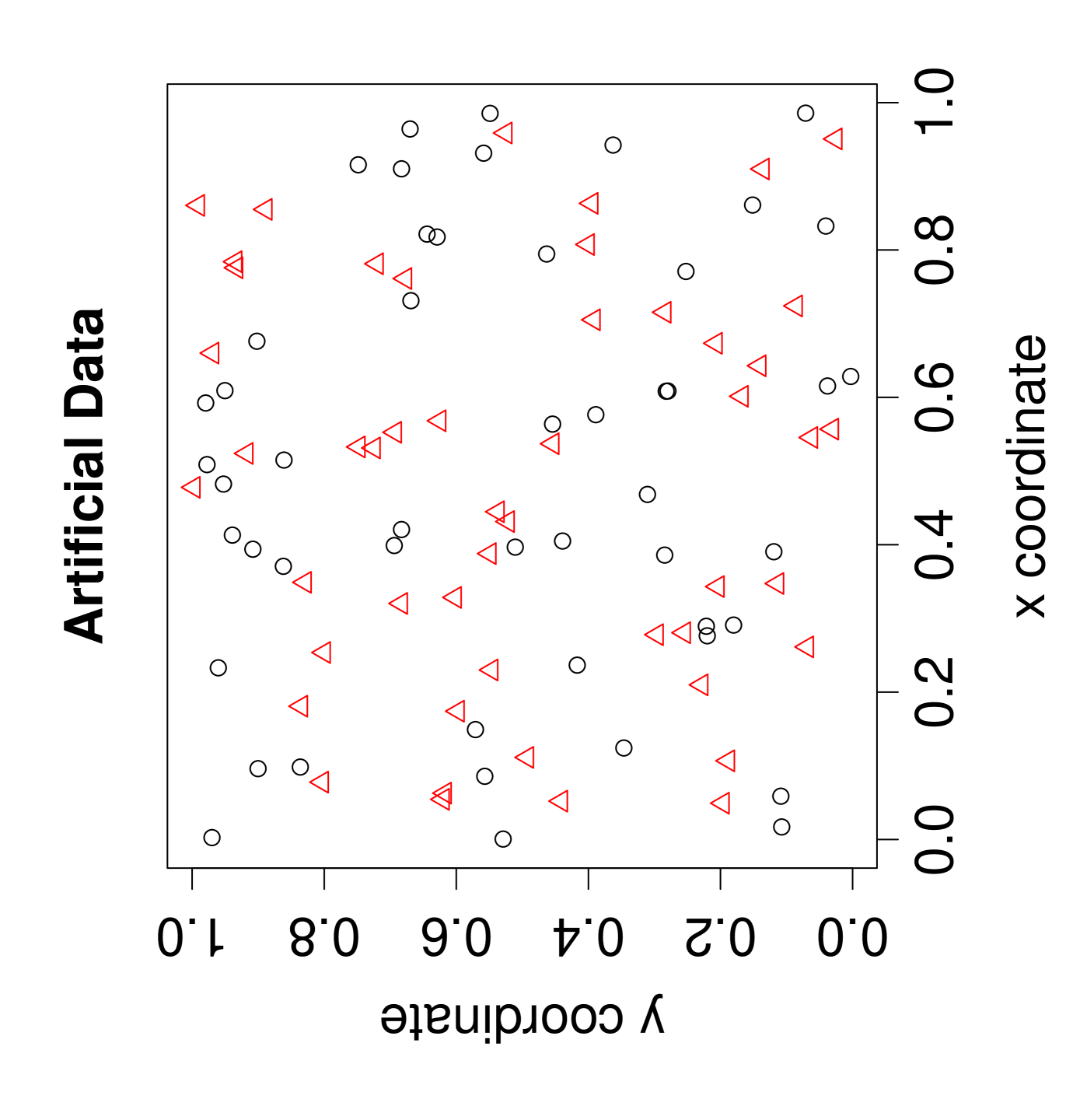
In the swamp tree example, although the test statistics for unadjusted and QR-adjusted versions are different for Pielou’s and Dixon’s tests and $p$-values for QR-adjusted versions are larger than unadjusted ones, I have the same conclusion: there is strong evidence for segregation of tree species. Below, I present an artificial example, a random sample of size 100 (with $50$ $X$-points and $50$ $Y$-points uniformly generated on the unit square). The question of interest is the spatial interaction between $X$ and $Y$ classes. I plot the locations of the points in Figure 7 and the corresponding NNCT together with percentages are provided in Table 6. Observe that the percentages are suggestive of mild segregation, with equal degree for both classes.

The data is generated to resemble the CSR independence pattern, so I assume the null pattern is CSR independence, which implies that our inference will be a conditional one if I use the observed values of $Q$ and $R$. I observe $Q=70$ and $R=60$ for this data set, and the empirical estimates for these sample sizes are $Q=63.37$ and $R=62.17$. I present the tests statistics and the associated $p$-values for NNCT-tests in Table 6. Observe that the test statistics all decrease with the QR-adjustment, however this decrease is not substantial to alter the conclusions. Based on the NNCT-tests, I find that the spatial interaction between $X$ and $Y$ is not significantly different from CSR independence.

In both examples although QR-adjustment did not change the conclusions, it might make a difference if the pattern is a close call between CSR independence and segregation/association. That is, if a segregation test has a $p$-value about .05, after the QR-adjustment, it might get to be significant or insignificant, depending on the case.

References

- Ceyhan, (2006) Ceyhan, E. (2006). On the use of nearest neighbor contingency tables for testing spatial segregation. Accepted for publication in Environmental and Ecological Statistics.
- Ceyhan, (2007) Ceyhan, E. (2007). New tests for spatial segregation based on nearest neighbor contingency tables. Under review.
- Cuzick and Edwards, (1990) Cuzick, J. and Edwards, R. (1990). Spatial clustering for inhomogeneous populations (with discussion). Journal of the Royal Statistical Society, Series B, 52:73–104.
- Diggle, (2003) Diggle, P. J. (2003). Statistical Analysis of Spatial Point Patterns. Hodder Arnold Publishers, London.
- Dixon, (1994) Dixon, P. M. (1994). Testing spatial segregation using a nearest-neighbor contingency table. Ecology, 75(7):1940–1948.
- Dixon, (2002) Dixon, P. M. (2002). Nearest-neighbor contingency table analysis of spatial segregation for several species. Ecoscience, 9(2):142–151.
- Good and Whipple, (1982) Good, B. J. and Whipple, S. A. (1982). Tree spatial patterns: South Carolina bottomland and swamp forests. Bulletin of the Torrey Botanical Club, 109:529–536.
- Goreaud and Pélissier, (2003) Goreaud, F. and Pélissier, R. (2003). Avoiding misinterpretation of biotic interactions with the intertype -function: population independence vs. random labelling hypotheses. Journal of Vegetation Science, 14(5):681 –692.
- Hamill and Wright, (1986) Hamill, D. M. and Wright, S. J. (1986). Testing the dispersion of juveniles relative to adults: A new analytical method. Ecology, 67(2):952–957.
- Herler and Patzner, (2005) Herler, J. and Patzner, R. A. (2005). Spatial segregation of two common Gobius species (Teleostei: Gobiidae) in the Northern Adriatic Sea. Marine Ecology, 26(2):121–129.
- Kulldorff, (2006) Kulldorff, M. (2006). Tests for spatial randomness adjusted for an inhomogeneity: A general framework. Journal of the American Statistical Association, 101(475):1289–1305.
- Meagher and Burdick, (1980) Meagher, T. R. and Burdick, D. S. (1980). The use of nearest neighbor frequency analysis in studies of association. Ecology, 61(5):1253–1255.
- Moran, (1948) Moran, P. A. P. (1948). The interpretation of statistical maps. Journal of the Royal Statistical Society, Series B, 10:243–251.
- Nanami et al., (1999) Nanami, S. H., Kawaguchi, H., and Yamakura, T. (1999). Dioecy-induced spatial patterns of two codominant tree species, Podocarpus nagi and Neolitsea aciculata. Journal of Ecology, 87(4):678–687.
- Orton, (1982) Orton, C. R. (1982). Stochastic process and archeological mechanism in spatial analysis. Journal of Archeological Science, 9:1–23.
- Pielou, (1961) Pielou, E. C. (1961). Segregation and symmetry in two-species populations as studied by nearest-neighbor relationships. Journal of Ecology, 49(2):255–269.
- Ripley, (2004) Ripley, B. D. (2004). Spatial Statistics. Wiley-Interscience, New York.
- Searle, (2006) Searle, S. R. (2006). Matrix Algebra Useful for Statistics. Wiley-Intersciences.
- Waller and Gotway, (2004) Waller, L. A. and Gotway, C. A. (2004). Applied Spatial Statistics for Public Health Data. Wiley-Interscience, NJ.
- Whipple, (1980) Whipple, S. A. (1980). Population dispersion patterns of trees in a Southern Louisiana hardwood forest. Bulletin of the Torrey Botanical Club, 107:71–76.