Temperature Dependence of the Density and Excitations of Dipolar Droplets

Ultracold bosonic gases form almost ideal, dilute, weakly interacting quantum systems. At temperatures much lower than the condensation temperature nearly all atoms share the collective ground state wavefunction, and the effect of interactions can be accounted for by their self-consistent action on that wavefunction. This mean-field idea, captured by the Gross-Pitaevskii equation Pitaevskii (1961); Gross (1961), qualitatively describes all the equilibrium properties of almost all the trapped Bose gas experiments. The corrections to the dynamics described by GP equation arise from particles which are above the condensate. The effect of this condensate depletion is detectable, but remains small at low temperatures as long as the system remains dilute and weakly interacting.

An alternative scenario for equilibrium, in which the effect of fluctuations is crucial, can arise if the mean field interactions describe an unstable system. The instability in the mean field description can be cured by the inclusion of fluctuations, which remain small compared to mean field effects even when they provide stability. This scenario of fluctuation stabilized equilibrium was first suggested theoretically by Petrov Petrov (2015) for two component Bose mixtures, and recently observed experimentally Cabrera et al. (2018); Semeghini et al. (2018); D’Errico et al. (2019). For dipolar gases, droplet formation in the mean-field unstable regime was first reported experimentally, where follow-up experiments have definitively established the fluctuation based stabilization as their formation mechanism Kadau et al. (2016); Ferrier-Barbut et al. (2016); Schmitt et al. (2016); Chomaz et al. (2016).

The theoretical description of the dipolar droplets have so far Wächtler and Santos (2016, 2016); Bisset and Blakie (2015); Bisset et al. (2016); Baillie et al. (2016) relied on the generalized Gross Pitaevskii equation for the condensate wave function

$$\left[-\frac{\hbar^{2}\nabla^{2}}{2m}+U_{tr}(\mathbf{x})+\int d^{3}\textbf{x}^{\prime}V_{\text{int}}(\textbf{x},\textbf{x}^{\prime})|\Psi(\textbf{x}^{\prime})|^{2}\right]\Psi(\mathbf{x})\\ =\left(\mu-\Delta\mu_{QF}(\mathbf{x})\right)\Psi(\mathbf{x}),$$

(1)

where the usual GP equation is modified by the quantum fluctuation contribution to chemical potential $\Delta\mu_{QF}(\mathbf{x})$. This contribution is then assumed to be determined entirely in terms of the local condensate wavefunction as it would be found in a uniform gas

$$\Delta\mu_{QF}(\Psi(\mathbf{x}))\propto|\Psi(\mathbf{x})|^{3}.$$

(2)

The exact coefficient linking $|\Psi|^{3}$ to $\Delta\mu_{QF}$ depends on the infrared cutoff choice used the in the local density approximation, but all different choices used in the literature for this cutoff give results which are in agreement with observations within experimental accuracy.

In a recent paper Aybar and Oktel (2019), we showed that the modified GP equation can be derived using the Hartree-Fock-Bogoliubov theory (HFBT) Griffin (1996) together with local density approximation for fluctuations. Such a treatment makes the assumptions underlying the generalized GP equation more transparent. We found that the above form of the generalized GP equation is valid only when the Hartree potential created by the depleted particles is negligible. This condition is satisfied in the dipolar droplet experiments, where the estimates for the number of depleted particles remain small even in the droplet regime.

The novel physical regime probed in the droplet experiments is evident in this set of approximations, as the number of depleted particles is negligible compared to the number of condensed particles, but their interaction with the condensate wavefunction supply the energy cost required for stability.

The derivation of the generalized GP equation from HFBT can be carried out at finite temperature Aybar and Oktel (2019); Boudjemâa (2017) without further complications. Quantum fluctuations are supplemented by thermal fluctuations, and in general the dynamics of such a system should be given in terms of a two fluid model with separate equations for the condensate and normal components. However, at low enough temperatures, the total number of depleted atoms would still be much smaller than the number of atoms in the condensate, and the dynamics of the fluctuations can be described only in terms of the local condensate wavefunction. Thus, a finite temperature version of the generalized GP equation was derived in which local chemical potential correction is now a function of both the condensate density and the temperature $\Delta\mu_{QF}(\Psi(\mathbf{x}),T)$. We solved this equation with a Gaussian variational ansatz and found that even if the temperature depletion remains small, the condensate density may be strongly modified. The change in the local compressibility is particularly pronounced near the first order transition to the droplet state.

In this paper, we first verify the conclusions obtained in Ref.Aybar and Oktel (2019), with a numerical solution of the generalized GP equation. We investigate the effects of temperatures which are much smaller than the BEC transition temperature, so that the thermal depletion density is much smaller than the condensate density but comparable to the quantum depletion. This temperature regime is likely to be relevant for both the Dy experiments by the Stuttgart group Kadau et al. (2016); Ferrier-Barbut et al. (2016); Schmitt et al. (2016), and the Er experiments by the Innsbruck group Chomaz et al. (2016). Our numerical results show that the effect of temperature on the density is most prominent for sudden transitions to the droplet states as obtained for initially oblate (pancake) clouds. For cigar shaped (prolate) clouds, the transition to the droplet state is smooth, and the effect of temperature remains small throughout the transition. Based on this observation, we investigate whether collective oscillation frequencies show any dependence on temperature at these low temperatures. We use both an effective Lagrangian based on a Gaussian ansatz, and real time numerical evolution to investigate the lowest lying collective excitations of the droplet state. We find that the collective oscillation frequencies show strong dependence on temperature close to the first order transition.

In the next section, we briefly summarize our HFBT method and give the resulting temperature dependent generalized GP equation. Section III explains our numerical algorithm and gives the calculated equilibrium density profiles for the Er and Dy experiments. Section IV contains the temperature dependence of the lowest collective oscillation frequencies of the condensate obtained by both a variational Lagrangian method and numerical real time evolution. A summary of the results and their relevance for the experiments on dipolar droplets are given in section V.

We consider Bosonic atoms of mass $M$ in a confining potential $U_{\text{tr}}(\mathbf{x})$ with chemical potential $\mu$, described by the Hamiltonian

	$\displaystyle\hat{H}$	$\displaystyle=$	$\displaystyle\int d^{3}\mathbf{x}\hat{\psi}^{\dagger}(\mathbf{x})\left(-\frac{\hbar^{2}\nabla^{2}}{2M}+U_{\text{tr}}(\mathbf{x})-\mu\right)\hat{\psi}(\mathbf{x})$
		$\displaystyle+$	$\displaystyle\frac{1}{2}\iint d^{3}\mathbf{x}d^{3}\mathbf{x}^{\prime}\hat{\psi}^{\dagger}(\mathbf{x})\hat{\psi}^{\dagger}(\mathbf{x}^{\prime})V_{\text{int}}(\mathbf{x}-\mathbf{x}^{\prime})\hat{\psi}(\mathbf{x}^{\prime})\hat{\psi}(\mathbf{x}),$

with the Bosonic commutation $[\hat{\psi}(\mathbf{x}),\hat{\psi}^{\dagger}(\mathbf{x}^{\prime})]=\delta(\mathbf{x}-\mathbf{x}^{\prime})$ of field operators. The interaction potential between the particles have both a short range, and a long range (dipolar) part

$$V_{\text{int}}(\mathbf{x})=g\left[\delta(\mathbf{x})+\frac{3\epsilon_{dd}}{4\pi|\mathbf{x}|^{3}}\left(1-3\frac{z^{2}}{|\mathbf{x}|^{2}}\right)\right],$$

(4)

where the short range repulsion is expressed in terms of the s-wave scattering length $a_{s}$ as $g=4\pi\hbar^{2}a_{s}/M$ and the relative strength of the dipolar interaction defines the dimensionless parameter $\epsilon_{dd}$.

We consider systems where most of the atoms occupy the condensate state. The total particle number $N$ is set by the chemical potential and $N_{0}$, the largest eigenvalue of the one particle density matrix $\langle\hat{\psi}^{\dagger}\hat{\psi}\rangle$ is close to this number $N-N_{0}\ll N$. The part of the field operator corresponding to the condensate can then be safely approximated by the classical field $\Psi(\textbf{x})$, the condensate wavefunction. The remaining part, which is referred to as the fluctuation operator, $\hat{\phi}(\textbf{x})=\hat{\psi}(\textbf{x})-\Psi(\textbf{x})$ can be used to define the one particle non-condensate density matrices. The direct non-condensate density is

$$\tilde{n}(\textbf{x}^{\prime},\textbf{x})=\langle\hat{\phi}^{\dagger}(\textbf{x}^{\prime})\hat{\phi}(\textbf{x})\rangle,$$

(5)

and the anomalous non-condensate density is

$$\tilde{m}(\textbf{x}^{\prime},\textbf{x})=\langle\hat{\phi}(\textbf{x}^{\prime})\hat{\phi}(\textbf{x})\rangle.$$

(6)

The aim of HFBT is to reduce the Hamiltonian to a system of self-consistent equations which describe the equilibrium values for the condensate wavefunction $\Psi(\textbf{x})$ and the non-condensate densities $\tilde{n},\tilde{m}$ Griffin (1996). This is achieved by assuming that the higher order correlation functions can be factorized in terms of these three quantities, e.g.

$$\hat{\phi}^{\dagger}(\textbf{x})\hat{\phi}^{\dagger}(\textbf{x}^{\prime})\hat{\phi}(\textbf{x}^{\prime})\approx\tilde{m}^{*}(\textbf{x}^{\prime},\textbf{x})\hat{\phi}(\textbf{x}^{\prime})+\tilde{n}^{*}(\textbf{x}^{\prime},\textbf{x})\hat{\phi}^{\dagger}(\textbf{x}^{\prime})+\tilde{n}(\textbf{x}^{\prime})\hat{\phi}^{\dagger}(\textbf{x}).$$

(7)

This procedure yields the GP equation

$$\mathcal{L}\Psi(\textbf{x})+\int d^{3}\textbf{x}^{\prime}V_{\text{int}}(\textbf{x}-\textbf{x}^{\prime})\tilde{n}(\textbf{x}^{\prime},\textbf{x})\Psi(\textbf{x}^{\prime})+\int d^{3}\textbf{x}^{\prime}V_{\text{int}}(\textbf{x}-\textbf{x}^{\prime})\tilde{m}(\textbf{x}^{\prime},\textbf{x})\Psi^{*}(\textbf{x}^{\prime})=0,$$

(8)

where $\mathcal{L}=\left[-\hbar^{2}\nabla^{2}/2M-\mu+U_{\text{tr}}(\textbf{x})+\int d^{3}\textbf{x}^{\prime}V_{\text{int}}(\textbf{x}-\textbf{x}^{\prime})|\Psi(\textbf{x}^{\prime})|^{2}+\int d^{3}\textbf{x}^{\prime}V_{\text{int}}(\textbf{x}-\textbf{x}^{\prime})\tilde{n}(\textbf{x}^{\prime})\right],$ displaying the dependence of the condensate wavefunction on the non-condensate densities.

To complete the self consistent loop, non-condensate densities must be calculated in terms of the condensate wavefunction. This is achieved by obtaining the Bogoliubov-DeGennes (BdG) equations for excitations,

$$\begin{split}\mathcal{L}_{0}u_{j}(\textbf{x})+\int d^{3}\textbf{x}^{\prime}V_{\text{int}}(\textbf{x}-\textbf{x}^{\prime})\Psi^{*}(\textbf{x}^{\prime})\Psi(\textbf{x})u_{j}(\textbf{x}^{\prime})-\int d^{3}\textbf{x}^{\prime}V_{\text{int}}(\textbf{x}-\textbf{x}^{\prime})\Psi(\textbf{x}^{\prime})\Psi(\textbf{x})v_{j}(\textbf{x}^{\prime})=E_{j}u_{j}(\textbf{x})\\ \mathcal{L}_{0}v_{j}(\textbf{x})+\int d^{3}\textbf{x}^{\prime}V_{\text{int}}(\textbf{x}-\textbf{x}^{\prime})\Psi(\textbf{x}^{\prime})\Psi^{*}(\textbf{x})v_{j}(\textbf{x}^{\prime})-\int d^{3}\textbf{x}^{\prime}V_{\text{int}}(\textbf{x}-\textbf{x}^{\prime})\Psi^{*}(\textbf{x}^{\prime})\Psi^{*}(\textbf{x})u_{j}(\textbf{x}^{\prime})=-E_{j}v_{j}(\textbf{x}),\end{split}$$

(9)

where $\mathcal{L}_{0}=\left[-\hbar^{2}\nabla^{2}/2M-\mu+U_{\text{tr}}(\textbf{x})+\int d^{3}\textbf{x}^{\prime}V_{\text{int}}(\textbf{x}-\textbf{x}^{\prime})|\Psi(\textbf{x}^{\prime})|^{2}\right].$ The solutions for the amplitudes $u,v$ can be summed to give the non-condensate densities

$$\begin{split}\tilde{n}(\textbf{x}^{\prime},\textbf{x})=&\sum_{j}\left(v_{j}(\textbf{x}^{\prime})v_{j}^{*}(\textbf{x})+N_{B}(E_{j})\left[u_{j}^{*}(\textbf{x}^{\prime})u_{j}(\textbf{x})+v_{j}(\textbf{x}^{\prime})v_{j}^{*}(\textbf{x})\right]\right)\\ \tilde{m}(\textbf{x}^{\prime},\textbf{x})=&-\sum_{j}\left(u_{j}(\textbf{x}^{\prime})v_{j}^{*}(\textbf{x})+N_{B}(E_{j})\left[v_{j}^{*}(\textbf{x}^{\prime})u_{j}(\textbf{x})+u_{j}(\textbf{x}^{\prime})v_{j}^{*}(\textbf{x})\right]\right).\end{split}$$

(10)

It is important to note here that we have ignored the interactions between the non-condensate particles in the above Eq.9, as we are interested at temperatures much lower than condensation temperature and the depletion remains small.

The calculation of non-condensate densities in terms of the condensate wavefunction in principle requires the determination of the full spectrum of the BdG equations. While the first few modes of these equations would have wavelengths close to the size of the system, the wavelength of the following BdG modes would get much smaller than the size of the system, or the coherence length of the condensate. For such modes the condensate density and the external trapping potential are slowly varying and Eq.9 can be solved with a local density approximation akin to the WKB approximation. Within this approximation, the non-condensate densities are locally determined in terms of the condensate wavefunction. The self consistency requirement can be stated only in terms of the condensate wavefunction, which yields the generalized GP equation.

At zero temperature, the condensate wavefunction then satisfies

$$\left[\left(-\frac{\hbar^{2}\nabla^{2}}{2M}+U_{\text{tr}}(\mathbf{x})-\mu\right)+\Phi_{H}(\mathbf{x})+\Omega_{n}(\mathbf{x})+\Omega_{m}(\mathbf{x})\right]\Psi(\mathbf{x})=0,$$

(11)

where the Hartree potential is $\Phi_{H}(\mathbf{x})=\int d^{3}\mathbf{x}^{\prime}V_{\text{int}}(\mathbf{x}-\mathbf{x}^{\prime})(|\Psi(\mathbf{x}^{\prime})|^{2}+\tilde{n}(\mathbf{x}^{\prime}))$. The local fluctuation induced potential, which is equivalent to the Lee-Huang-Yang correction has two contributions coming from direct and anomalous non-condensate densities,

	$\displaystyle\Omega_{n}(\textbf{x})\Psi(\textbf{x})$	$\displaystyle=$	$\displaystyle\frac{8}{3}gn_{0}(\textbf{x})\sqrt{\frac{a^{3}_{s}n_{0}(\textbf{x})}{\pi}}\mathcal{Q}_{5}(\epsilon_{dd})\Psi(\textbf{x}),$		(12)
	$\displaystyle\Omega_{m}(\textbf{x})\Psi(\textbf{x})$	$\displaystyle=$	$\displaystyle 8gn_{0}(\textbf{x})\sqrt{\frac{a^{3}_{s}n_{0}(\textbf{x})}{\pi}}\mathcal{Q}_{5}(\epsilon_{dd})\Psi(\textbf{x}),$

where $Q_{l}(\epsilon_{dd})=\int_{0}^{1}du[1+\epsilon_{dd}(3u^{2}-1)]^{l/2}$. Explicitly, this is almost the generalized GP equation used in the literature Wächtler and Santos (2016); Bisset et al. (2016),

$$\left[-\frac{\hbar^{2}\nabla^{2}}{2M}+U_{\text{tr}}(\mathbf{x})-\mu+\int d^{3}\mathbf{x}^{\prime}V_{\text{int}}(\mathbf{x}-\mathbf{x}^{\prime})\left(|\Psi(\mathbf{x}^{\prime})|^{2}+\tilde{n}(\mathbf{x}^{\prime})\right)+\frac{32}{3}g\sqrt{\frac{a^{3}_{s}}{\pi}}\mathcal{Q}_{5}(\epsilon_{dd})|\Psi(\mathbf{x})|^{3}\right]\Psi(\mathbf{x})=0.$$

(13)

Thus the only correction to the generalized GP equation obtained by adding local LHY correction to the chemical potential is the Hartree potential created by the depleted particles. If the depletion $\tilde{n}(\mathbf{x})=\frac{8}{3}\sqrt{\frac{a^{3}_{s}}{\pi}}\mathcal{Q}_{3}(\epsilon_{dd})|\Psi(\mathbf{x}^{\prime})|^{3}$ remains small, this contribution will be accordingly small.

If the dipolar interaction is not dominant, $\epsilon_{dd}<1$, the trapped gas will be stable at low densities and fluctuation contribution is not qualitatively important. However for strong dipolar interaction, $\epsilon_{dd}>1$, the gas has an instability towards collapse as the attractive part of the dipolar interaction can favor higher densities. The local fluctuation induced interaction potential can arrest this collapse as it scales with a higher power of the density, $n_{0}^{3/2}$, compared to the direct interaction with $n_{0}$. While this general physical mechanism has been tested experimentally Ferrier-Barbut et al. (2016) to be at play in the droplet experiments, the exact coefficient of the fluctuation term is not easy to determine. When $\epsilon_{dd}>1$ there is no stable solution for a uniform system, some long wavelength modes will have imaginary frequencies signaling collapse. Thus the expressions $\Omega_{n}$, and $\Omega_{m}$ (Eq. 12) will have imaginary parts. One approach in the literature was to ignore the imaginary components, assuming they only cause decay at long times Schmitt et al. (2016). However this imaginary part is clearly a by–product of the LDA, which as we have discussed above is valid only for higher Bogoliubov modes. A careful accounting of the discrete nature of the Bogoliubov modes would not show any imaginary frequencies, but a computationally much simpler approach is to impose a cutoff on which LDA modes should be taken into account as employed in RefWächtler and Santos (2016); Bisset et al. (2016). We used a spherical cutoff in k-space which excludes all modes with wavevectors smaller than $k_{c}=\frac{\pi}{2\xi}$, as the coherence length of the condensate $\xi$ is the length scale which characterizes locality for the condensate.

The systematic derivation of the generalized GP equation using HFBT enables straightforward generalization to finite temperatures. While the HFBT is mostly reliable at all temperatures, local calculation of non-condensate densities solely in terms of local condensate wavefunction puts a severe restriction on the applicability of LDA to obtain a generalized GP equation at non-zero temperature. The dynamics of condensate and non-condensate atoms are controlled by different equations, and only when the number of non-condensate atoms is small enough their dynamics will be completely determined by the condensate. At zero temperature this essentially means that the system is weakly interacting enough to limit quantum depletion. At finite temperature non-condensate density is contributed to by both quantum and thermal depletion mechanisms. The non-condensate part dynamics will be controlled completely by the condensate only if the total depletion remains small. Essentially, to be able to write a single self consistent equation for the condensate the temperature must be much smaller than the BEC transition temperature so that the thermal depletion is comparable to the quantum depletion.

At such low but non-zero temperatures, the generalized GP equation takes the similar form

$$\left[-\frac{\hbar^{2}\nabla^{2}}{2m}+U_{tr}(\mathbf{x})+\int d^{3}\textbf{x}^{\prime}V_{\text{int}}(\textbf{x}-\textbf{x}^{\prime})|\Psi(\textbf{x}^{\prime})|^{2}\right]\Psi(\mathbf{x})+\Delta\mu_{QF}(\mathbf{x},T)\Psi(\mathbf{x})=\mu\Psi(\mathbf{x}),$$

(14)

with temperature only playing a role in the determination of the local fluctuation induced interaction. With the same cutoff used at zero temperature we obtain

$$\Delta\mu_{QF}(\mathbf{x},T)=\frac{32}{3}g\sqrt{\frac{a_{s}^{3}}{\pi}}\left(\mathcal{Q}_{5}(\epsilon_{dd})+\mathcal{R}(\epsilon_{dd},t(\mathbf{x}))\right)|\Psi(\textbf{x})|^{3},$$

(15)

with dimensionless temperature $t=k_{B}T/gn_{0}(\mathbf{x})$ and

$$\mathcal{Q}_{5}(\epsilon_{dd};q_{c})=\frac{1}{4\sqrt{2}}\int_{0}^{1}duf(u)\left[\left(4f(u)-q_{c}^{2}\right)\sqrt{2f(u)+q_{c}^{2}}-3f(u)q_{c}+q_{c}^{3}\right]$$

(16)

$$\mathcal{R}(\epsilon_{dd},t;q_{c})=\frac{3}{4\sqrt{2}}\int_{0}^{1}du\int_{q_{c}^{2}}^{\infty}dQ\frac{Qf(u)}{\sqrt{Q+2f(u)}}\frac{1}{\exp[\sqrt{Q\left(Q+2f(u)\right)}/t]-1}.$$

(17)

In Ref. Aybar and Oktel (2019) we calculated these dimensionless functions, and obtained a $t^{2}$ power law fit $\mathcal{R}(\epsilon_{dd},t)=S(\epsilon_{dd})t^{2}$ and the coefficient is best approximated by $\mathcal{S}(\epsilon_{dd})=-0.01029\epsilon_{dd}^{4}+0.02963\epsilon_{dd}^{3}-0.05422\epsilon_{dd}^{2}+0.009302\epsilon_{dd}+0.1698$ for $0<\epsilon_{dd}<2$.

We now discuss the numerical solution of Eq.14 with the parametrization in the previous section, and compare it with the variational solution presented in Ref.Aybar and Oktel (2019). Our focus is on the observable effects of temperature on the density profile. As our LDA approach neglects the effect of interactions of the non-condensate atoms the temperature range will be limited so as to make sure that the condensate fraction remains close to one.

We use time splitting spectral method Bao et al. (2003) to evolve the GP equation in imaginary time until convergence in energy is reached. A three dimensional grid of up to 64 by 64 by 256 points in real space is used to capture the anisotropic shape of the droplets, where the real space discretization step is determined to ensure smooth variation of the cloud density.

The Hartree potential created by the long range dipolar interaction is calculated by expressing it as a convolution in k space.

$$V_{H}^{(dd)}(\mathbf{x})=\int\frac{d^{3}\mathbf{k}}{\left(2\pi\right)^{3}}\tilde{n}_{0}(\mathbf{k})\tilde{V}_{dd}(\mathbf{k})e^{i\mathbf{k}\cdot\mathbf{x}},$$

(18)

where the Fourier transform of the dipolar interaction is

$$\tilde{V}_{dd}(\mathbf{k})=\epsilon_{dd}\left(3\frac{k_{z}^{2}}{|\mathbf{k}|^{2}}-1\right).$$

(19)

While this expression avoids the complications of the dipolar potential near zero separation the use of discrete Fourier transforms instead of the continuum integrals effectively introduces repeated copies of the simulation cell. In order to avoid the interaction between neighboring real space cells we used a spherical cutoff on the dipolar interaction which sets the interaction to zero beyond the cutoff distance. This cutoff distance must be chosen larger than the maximum size of the droplet so that the points at the edges of the cigar shaped cloud interact with each other. However, it must be shorter than then the distance between the closest points of clouds in spuriously repeated simulation cells, so that long range interactions take place only within one simulation cell. We choose the size of the simulation cell and the cutoff to comply with these constraints. The Fourier transform of the dipolar potential with this cutoff is calculated as

$$\tilde{V}_{dd}^{(cut)}(\mathbf{k})=\tilde{V}_{dd}(\mathbf{k})\left(1-3\frac{\sin\left(|\mathbf{k}|R\right)-|\mathbf{k}|R\cos\left(|\mathbf{k}|R\right)}{\left(|\mathbf{k}|R\right)^{3}}\right)$$

(20)

After numerically obtaining the solution, we extract the widths using the moments such that they correspond to the variational width parameters when applied to a variational Gaussian state Bisset and Blakie (2015),

	$\displaystyle\sigma_{\rho}^{2}=\frac{4}{N}\int d^{3}\mathbf{x}\rho^{2}|\Psi(\mathbf{x})|^{2},$		(21)
	$\displaystyle\sigma_{z}^{2}=\frac{2}{N}\int d^{3}\mathbf{x}z^{2}|\Psi(\mathbf{x})|^{2}.$

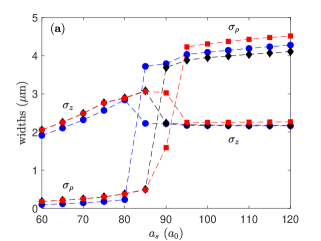
We first consider a parameter regime for which there is a sharp transition from a pancake shaped low density cloud to a single droplet. Focusing on the parameter regime explored in the Stuttgart experiments Kadau et al. (2016); Ferrier-Barbut et al. (2016); Schmitt et al. (2016), we calculate the density profile for $N=2000$ Dy atoms in an axially symmetric trap with frequencies $f_{\perp}=45$Hz, $f_{z}=133$Hz. At zero temperature the cloud enters the droplet state below $a_{c}^{(0)}=83a_{0}$. As can be seen in Fig.1, increasing temperature shifts this transition to higher scattering lengths, where a 100nK change in the cloud temperature can be observed to make a $\sim 10a_{0}$ change in the transition point. It is possible to induce the transition from the cloud to the droplet by increasing the temperature as shown in Fig 1, for $a_{s}=88a_{0}$ the cloud enters the droplet state around $T\simeq 110nK$.

We see from our derivation that there are three effects of raising the temperature in a dipolar droplet system. First effect will be that the LHY term increases as thermal fluctuations now supplement quantum fluctuations stabilizing the droplet state. The second effect is that the number of particles in the condensate is lowered because of the thermal depletion, and following this the third effect is that the depleted particle density will have long range dipolar interactions with the condensate. Our calculations show that at the lowest temperatures which are relevant for the current experiments the change in the compressibility of the droplet, i.e. the LHY term, will be the most dominant of these three effects. However, even though the temperature contribution to LHY term is always positive, its effect on the transition between the low density and the droplet state is non-trivial.

Let’s particularly focus on the pancake shape traps for which the distinction between the droplet and low density phases is sharp. The attractive part of the dipolar interaction favors higher density and higher aspect ratios for the cloud, which would normally collapse the cloud for $\epsilon_{DD}>1$. This inclination is resisted by two different mechanisms for the low density and droplet phases. In the low density phase the trap potential along the z direction combined with the short range repulsion stops the collapse. The effect of low temperature is negligible for the low density minimum. For the droplet phase the confining potential is irrelevant and the collapse is arrested by the LHY energy which increases with a higher power of density. The first effect of temperature is an increase in the coefficient of the LHY term.

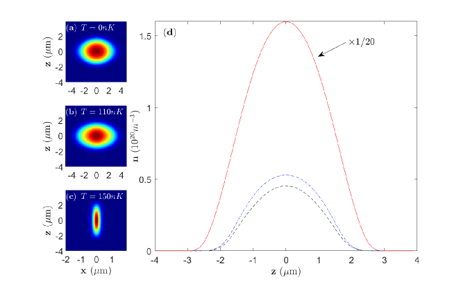
In a pancake trap the transition is first order, so the system chooses the local minimum with the lower energy. As temperature is increased the minimum energy corresponding to the low density phase barely changes, while the minimum energy for the droplet changes due to the change in the LHY term. While the LHY contribution to energy increases, the droplet aspect ratio, thus the negative contribution of the dipolar interaction energy also increases. Increasing temperature lowers the total energy of the droplet minimum, resulting in the transition to the droplet state seen in Fig.1. While we base this argument on the variational study in Aybar and Oktel (2019), numerical results obtained here show that the non-trivial effect of the temperature on the transition is not an artifact of the restrictions to Gaussian wavefunctions. The results of the numerical calculation are in good agreement with the variational calculation presented in ref.Aybar and Oktel (2019). As can be seen Fig.2 even though the density of the center changes by a factor of $\simeq 20$ the profile of the cloud remains well approximated by a Gaussian throughout the transition, thus the variational fits retain their predictive power.

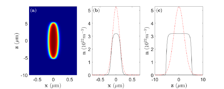
We also simulate what happens in the deep droplet state as can be seen in Fig. 3, the density profile is not a Gaussian any more, and the numerical solution is different from the variational result. The effect of low temperatures on this strong droplet state remains negligible.

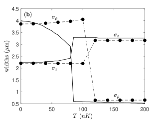
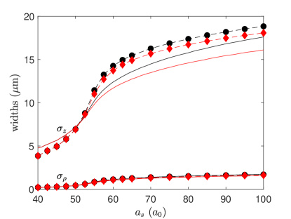
Next, we investigate a parameter regime for which the transition between the droplet and low-density phases is smooth, as observed in the Innsbruck experiments Ref. Chomaz et al. (2016). For $20000$ Er atoms in a trap with frequencies $f_{\perp}=178$Hz, $f_{z}=17.2$Hz the transition to the droplet is a continuous crossover near $a_{s}\simeq 50a_{0}$. We find that the temperatures up to $200nK$ have a distinct, yet small, effect on the cloud radii throughout, as can be seen in Fig. 4. Once again the density profile of the cloud remains Gaussian throughout the transition and the variational results are in good agreement with the numerical calculations.

Collective oscillations of trapped condensates have emerged as one of the most valuable experimental probes from the earliest experiments on ultracold atoms. Similarly, thermal activation of collective modes for superfluid Helium droplets were investigated Dalfovo and Stringari (2001) . The collective excitation frequencies of a trapped cloud reveal information about the equilibrium state and are in general sensitive to local compressibility of the system. For a short range interacting BEC, the collective oscillation frequencies are only weakly dependent on temperature except near the BEC critical temperature Jin et al. (1997). However, the dipolar droplet state is stabilized by fluctuations and the equilibrium can be more sensitive to thermal effects.

The oscillation modes for a dipolar gas at zero temperature has been calculated in Ronen et al. (2006). For the droplet state the lowest lying oscillation modes have been calculated in Wächtler and Santos (2016) by a variational approach, while the more general spectrum of excited modes of the droplet have been explored numerically by Baillie et al. (2016). The oscillation frequencies have been measured for Er droplets Chomaz et al. (2016), where the signature of the local LHY correction was clearly identified in the axial oscillation mode frequency. Similarly, collective oscillations in Dy droplets have been excited by tilting the dipole orientations Ferrier-Barbut et al. (2018).

We explore the few lowest lying modes of the droplet through both approaches. First, we write a variational Lagrangian for a Gaussian wavefunction for which coupled oscillations of the cloud width in three dimensions give us the lowest three modes of the condensate. We compare the values found from this approach with numerical real time evolution of the condensate.

We use a Gaussian ansatz for the wavefunction,

	$\displaystyle\Psi(x,y,z,t)$	$\displaystyle=\frac{\sqrt{N}}{\pi^{3/4}\left(w_{x}(t)w_{y}(t)w_{z}(t)\right)^{1/2}}$		(22)
		$\displaystyle\exp\left[-\frac{1}{2}\left(\frac{x^{2}}{w_{x}(t)^{2}}+\frac{y^{2}}{w_{y}(t)^{2}}+\frac{z^{2}}{w_{z}(t)^{2}}\right)+i\left(x^{2}\beta_{x}(t)+y^{2}\beta_{y}(t)+z^{2}\beta_{z}(t)\right)\right]$		(23)

where the time dependent parameters $w_{x,y,z}$ give the cloud radii. The other variational parameters $\beta_{x,y,z}$ facilitate the mass current so that the cloud density can oscillate. Such a restricted form for the variational wavefunction can only capture the three collective oscillation frequencies of the condensate. However, these lowest modes have been the most accessible modes experimentally and variational Lagrangian method results have been in good agreement with measurements Chomaz et al. (2016); Wächtler and Santos (2016).

For elongated cigar shape condensates such as the dipolar droplets, one of these modes feature oscillations predominantly in the axial direction. This axial mode has the lowest frequency which has been measured in Er and Dy experiments. The other two modes consist of breathing and quadrupolar excitations perpendicular to the long axis and typically have frequencies an order of magnitude larger than the axial mode for the droplets.

The effect of the beyond mean field correction for the oscillation frequencies have first been reported in Wächtler and Santos (2016). We now introduce the temperature dependence into the LHY correction. Our Lagrangian is:

	$\displaystyle\mathcal{L}=$	$\displaystyle\frac{i\hbar}{2}\left(\Psi(\mathbf{x},t)\frac{\partial\Psi^{*}(\mathbf{x},t)}{\partial t}-\Psi^{*}(\mathbf{x},t)\frac{\partial\Psi(\mathbf{x},t)}{\partial t}\right)+\frac{\hbar^{2}}{2M}|\nabla\Psi(\mathbf{x},t)|^{2}$		(24)
		$\displaystyle+U_{\text{tr}}(\mathbf{x})|\Psi(\mathbf{x},t)|^{2}$
		$\displaystyle+\frac{1}{2}\int d^{3}\mathbf{x^{\prime}}|\Psi(\mathbf{x},t)|^{2}V_{\text{int}}(\mathbf{x}-\mathbf{x^{\prime}})|\Psi(\mathbf{x^{\prime}},t)|^{2}$
		$\displaystyle+\frac{2}{5}\gamma|\Psi(\mathbf{x},t)|^{5}$
		$\displaystyle+2\theta T^{2}|\Psi(\mathbf{x},t)|,$

where $\gamma=\frac{32}{3}g\sqrt{\frac{a_{s}^{3}}{\pi}}\mathcal{Q}_{5}(\epsilon_{dd})$, and $\theta=\frac{32}{3}g\sqrt{\frac{a_{s}^{3}}{\pi}}\frac{k_{B}^{2}}{g^{2}}\mathcal{S}(\epsilon_{dd})$

The integrals in the Lagrangian can be carried out for the variational wavefunction to yield the Lagrangian in terms of the variational parameters as

	$\displaystyle L(w_{x},w_{y},w_{z},\beta_{x},\beta_{y},\beta_{z})=$	$\displaystyle\frac{N\hbar}{2}\left(w_{x}^{2}\dot{\beta}_{x}+w_{y}^{2}\dot{\beta}_{y}+w_{z}^{2}\dot{\beta}_{z}\right)$		(25)
		$\displaystyle+\frac{\hbar^{2}N}{4M}\left(\frac{1}{w_{x}^{2}}+\frac{1}{w_{y}^{2}}+\frac{1}{w_{z}^{2}}+4w_{x}^{2}\beta_{x}^{2}+4w_{y}^{2}\beta_{y}^{2}+4w_{z}^{2}\beta_{z}^{2}\right)$
		$\displaystyle+\frac{1}{4}MN\left(\omega_{x}^{2}w_{x}^{2}+\omega_{y}^{2}w_{y}^{2}+\omega_{z}^{2}w_{z}^{2}\right)$
		$\displaystyle+\frac{gN^{2}}{2}\frac{1}{2^{3/2}\pi^{3/2}w_{x}w_{y}w_{z}}\left(1-\epsilon_{dd}F\left(\frac{w_{x}}{w_{z}},\frac{w_{y}}{w_{z}}\right)\right)$
		$\displaystyle+\frac{4\sqrt{2}}{25\sqrt{5}\pi^{9/4}}\frac{N^{5/2}\gamma}{\left(w_{x}w_{y}w_{z}\right)^{3/2}}$
		$\displaystyle+4\sqrt{2}\pi^{3/4}\theta T^{2}N^{1/2}\left(w_{x}w_{y}w_{z}\right)^{1/2}.$

where

$$F(\kappa_{x},\kappa_{y})=1-3\kappa_{x}\kappa_{y}\int_{0}^{\pi}\frac{d\phi}{\pi}\left(\frac{\tanh^{-1}\left[\sqrt{1-\left(\kappa_{x}^{2}\cos^{2}\phi+\kappa_{y}^{2}\sin^{2}\phi\right)}\right]}{\left(1-\left(\kappa_{x}^{2}\cos^{2}\phi+\kappa_{y}^{2}\sin^{2}\phi\right)\right)^{3/2}}-\frac{1}{1-\left(\kappa_{x}^{2}\cos^{2}\phi+\kappa_{y}^{2}\sin^{2}\phi\right)}\right).$$

(26)

The Euler Lagrange equations for the radii give:

$$\hbar w_{\eta}\dot{\beta}_{\eta}+\frac{2\hbar^{2}}{M}w_{\eta}\beta_{\eta}^{2}+\frac{\partial G}{\partial w_{\eta}}=0,$$

(27)

while the phase terms are simply related to the velocity of the radii as

$$\beta_{\eta}=\frac{M}{2\hbar w_{\eta}}\dot{w}_{\eta},$$

(28)

where,

	$\displaystyle G(w_{x},w_{y},w_{z})=$	$\displaystyle\frac{\hbar^{2}}{4M}\left(\frac{1}{w_{x}^{2}}+\frac{1}{w_{y}^{2}}+\frac{1}{w_{z}^{2}}\right)+\frac{1}{4}M\left(\omega_{x}^{2}w_{x}^{2}+\omega_{y}^{2}w_{y}^{2}+\omega_{z}^{2}w_{z}^{2}\right)$		(29)
		$\displaystyle+\frac{gN}{2}\frac{1}{2^{3/2}\pi^{3/2}w_{x}w_{y}w_{z}}\left(1-\epsilon_{dd}F\left(\frac{w_{x}}{w_{z}},\frac{w_{y}}{w_{z}}\right)\right)$
		$\displaystyle+\frac{4\sqrt{2}}{25\sqrt{5}\pi^{9/4}}\frac{N^{3/2}\gamma}{\left(w_{x}w_{y}w_{z}\right)^{3/2}}+4\sqrt{2}\pi^{3/4}\theta T^{2}N^{-1/2}\left(w_{x}w_{y}w_{z}\right)^{1/2}.$

Therefore,

$$\frac{d^{2}w_{\eta}}{dt^{2}}=-\frac{2}{M}\frac{\partial}{\partial w_{\eta}}G(w_{x},w_{y},w_{z}).$$

(30)

We non-dimensionalize the equations in terms of the effective trap frequency $\bar{\omega}=\left(\omega_{x}\omega_{y}\omega_{z}\right)^{1/3}$, and the harmonic oscillator length $\bar{l}=\sqrt{\frac{\hbar}{M\bar{\omega}}}$. With $\nu_{i}=w_{i}/\bar{l}$, $\tau=\bar{\omega}t$ and $E_{0}=\hbar\bar{\omega}$, the effective potential $\tilde{U}$ becomes

	$\displaystyle\tilde{U}=$	$\displaystyle\frac{1}{2}\left(\frac{1}{\nu_{x}^{2}}+\frac{1}{\nu_{y}^{2}}+\frac{1}{\nu_{z}^{2}}\right)+\frac{1}{2}\left(\frac{\omega_{x}^{2}}{\bar{\omega}^{2}}\nu_{x}^{2}+\frac{\omega_{y}^{2}}{\bar{\omega}^{2}}\nu_{y}^{2}+\frac{\omega_{z}^{2}}{\bar{\omega}^{2}}\nu_{z}^{2}\right)$		(31)
		$\displaystyle+\sqrt{\frac{2}{\pi}}\frac{Na_{s}}{\bar{l}}\frac{1}{\nu_{x}\nu_{y}\nu_{z}}\left(1-\epsilon_{dd}F\left(\frac{\nu_{x}}{\nu_{z}},\frac{\nu_{y}}{\nu_{z}}\right)\right)$
		$\displaystyle+\mathbf{c}_{1}\frac{N^{3/2}a_{s}^{5/2}}{\bar{l}^{5/2}}\frac{1}{\left(\nu_{x}\nu_{y}\nu_{z}\right)^{3/2}}\mathcal{Q}_{5}(\epsilon_{dd})$
		$\displaystyle+\mathbf{c}_{2}\frac{a_{s}^{1/2}}{N^{1/2}\bar{l}^{1/2}}\left(\nu_{x}\nu_{y}\nu_{z}\right)^{1/2}\tilde{t}^{2}\mathcal{S}(\epsilon_{dd}),$

where $\mathbf{c}_{1}=\frac{1024\sqrt{2}}{75\sqrt{5}\pi^{7/4}}\approx 1.1648$, and $\mathbf{c}_{2}=\frac{64\sqrt{2}}{3\pi^{3/4}}\approx 12.785$. The equilibrium radii are found at the stationary point of the effective potential

$$\left.\frac{\partial\tilde{U}}{\partial\nu_{\eta}}\right|_{\nu_{\eta(0)}}=0.$$

(32)

Taylor expansion to second order near the equilibrium point defines the Hessian matrix

$$M=\begin{bmatrix}k_{x}&\lambda_{xy}&\lambda_{zx}\\ \lambda_{xy}&k_{y}&\lambda_{yz}\\ \lambda_{zx}&\lambda_{yz}&k_{z}\end{bmatrix},$$

(33)

where $k_{\eta}=\left.\frac{\partial^{2}\tilde{U}}{\partial\nu_{\eta}^{2}}\right|_{(0)}$, $\lambda_{\alpha,\beta}=\left.\frac{\partial^{2}\tilde{U}}{\partial\nu_{\alpha}\partial\nu_{\beta}}\right|_{(0)}$. Collective frequencies are found via diagonalization of this matrix. We numerically calculate the derivatives near the equilibrium point and obtain the collective oscillation frequencies.

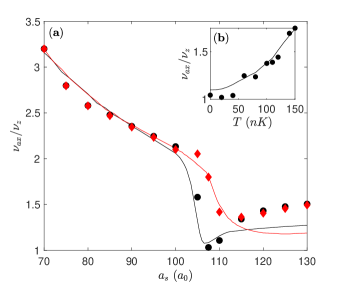
As a check on our variational results we also calculate the oscillation frequencies numerically through real time evolution with the split step method outlined in the previous section. We first calculate the oscillation frequencies for the Dy experimental parameters for which there is an abrupt transition. The oscillation frequencies increase upon transition to the droplet state, as can be seen in Fig.5. For $20000$ Dy atoms in a spherical trap with $f=75$Hz the transition takes place near $a_{s}\simeq 105a_{0}$ and is signalled by an abrupt change in the axial oscillation frequency. Repeating the same calculation for $T=150$nK we observe that the transition in the frequency becomes smoother as the transition point moves to higher $a_{s}$. Thus the most dramatic effect of temperature on the oscillation frequencies happens near the transition. The change in the frequency of the axial mode as a function of temperature is displayed in Fig. 5, where we observe close to 70% change near the critical $a_{s}=105a_{0}$. Both variational and numerical results give parallel physical pictures indicating that the increase in the oscillation frequency with temperature is greatest near the transition to the droplet state.

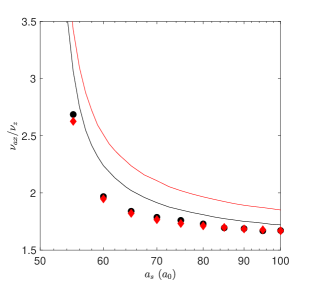
In the Er experiments the cigar shaped condensate has a smooth transition between the low density and droplet states. This smooth transition causes the cloud shape to be mostly immune to changes in temperature as explored in the previous section. Both the time dependent variational approach and the numerical real time evolution predict a sharp rise in the axial mode frequency upon droplet formation, which agree with the experimental observations in Ref.Chomaz et al. (2016). The variational approach predicts an increase in the oscillation frequencies with temperature as can be seen in Fig.6. However numerical solutions of the same equation show very little change from the zero temperature frequencies up to 150nK. As the droplet state is extremely elongated the variational approach may be overstating the importance of the compressibility of the center of the cloud by disregarding higher modes along the axial direction. Thus, we expect no significant low-temperature effect on the axial oscillation frequency close to smooth crossover to the droplet state.

In this paper we provide further support for the claim that dipolar droplets are particularly susceptible to thermal fluctuations at low temperatures. Numerical calculations presented here support the conclusions of the previous variational calculation Aybar and Oktel (2019). Furthermore, we show that the oscillation frequencies of collective modes are also sensitive to the temperature near the droplet transition. This should be expected as the collective modes are good probes of compressibility and the primary effect of temperature is to change the droplet’s local chemical potential.

Standard experimental methods for thermometry are not applicable to the current droplet experiments. The small size of the droplets impede the in-situ density measurement of the thermal component. Long range dipolar interactions affect the free expansion of the condensate, even when the droplet is not self-trapped Böttcher et al. (2019). The temperature data given in the literature is based on the thermal component before droplet formation for both the Dy Kadau et al. (2016) and the Er systems Chomaz et al. (2016). In the absence of reliable temperature measurement it is not possible to make a direct comparison of our results with the experimental data, either for Dy or Er experiments. Our results show that a change in the oscillation frequencies can occur even at temperatures much lower than the BEC transition temperature, and this may explain the uncertainty in the range of frequencies observed in Ferrier-Barbut et al. (2018); Chomaz et al. (2016). A change in the oscillation frequency for systems intentionally prepared at a higher temperature, or heated after droplet formation by an external probe would provide convincing evidence for the role of thermal fluctuations on dipolar droplets.

It is important to list the limitations of the approach used here. Our theory does not take the interactions between excited (above the condensate) particles into account, which limits it’s applicability to systems where the number of thermal atoms is close to the number of atoms in the condensate. Fluctuations are treated in the local density approximation, hence the independent dynamics of the thermal cloud is not considered. Furthermore, the expression for the local chemical potential suffers from an ad-hoc cutoff. These limitations make it hard to propose the collective oscillation frequencies as a quantitative measure of temperature. However, we believe that the dependence of the oscillation frequencies on temperature should be observable in the current experimental regime.

This project is supported by Türkiye Bilimsel ve Teknolojik Araştırma Kurumu (TÜBİTAK) Grant No. 116F215.

References

- Pitaevskii (1961) L. P. Pitaevskii, Zh. Eksp. Teor. Fiz. 40, 646 (1961).
- Gross (1961) E. P. Gross, “Structure of a quantized vortex in boson systems,” Il Nuovo Cimento (1955-1965) 20, 454–477 (1961).
- Petrov (2015) D. S. Petrov, “Quantum Mechanical Stabilization of a Collapsing Bose-Bose Mixture,” Phys. Rev. Lett. 115, 155302 (2015).
- Cabrera et al. (2018) C. R. Cabrera, L. Tanzi, J. Sanz, B. Naylor, P. Thomas, P. Cheiney, and L. Tarruell, “Quantum liquid droplets in a mixture of Bose-Einstein condensates,” Science 359, 301–304 (2018), publisher: American Association for the Advancement of Science Section: Report.
- Semeghini et al. (2018) G. Semeghini, G. Ferioli, L. Masi, C. Mazzinghi, L. Wolswijk, F. Minardi, M. Modugno, G. Modugno, M. Inguscio, and M. Fattori, “Self-bound quantum droplets of atomic mixtures in free space,” Phys. Rev. Lett. 120, 235301 (2018).
- D’Errico et al. (2019) C. D’Errico, A. Burchianti, M. Prevedelli, L. Salasnich, F. Ancilotto, M. Modugno, F. Minardi, and C. Fort, “Observation of quantum droplets in a heteronuclear bosonic mixture,” Phys. Rev. Research 1, 033155 (2019).
- Kadau et al. (2016) Holger Kadau, Matthias Schmitt, Matthias Wenzel, Clarissa Wink, Thomas Maier, Igor Ferrier-Barbut, and Tilman Pfau, “Observing the Rosensweig instability of a quantum ferrofluid,” Nature 530, 194–197 (2016).
- Ferrier-Barbut et al. (2016) Igor Ferrier-Barbut, Holger Kadau, Matthias Schmitt, Matthias Wenzel, and Tilman Pfau, “Observation of Quantum Droplets in a Strongly Dipolar Bose Gas,” Phys. Rev. Lett. 116, 215301 (2016).
- Schmitt et al. (2016) Matthias Schmitt, Matthias Wenzel, Fabian Böttcher, Igor Ferrier-Barbut, and Tilman Pfau, “Self-bound droplets of a dilute magnetic quantum liquid,” Nature 539, 259–262 (2016).
- Chomaz et al. (2016) L. Chomaz, S. Baier, D. Petter, M. J. Mark, F. Wächtler, L. Santos, and F. Ferlaino, “Quantum-Fluctuation-Driven Crossover from a Dilute Bose-Einstein Condensate to a Macrodroplet in a Dipolar Quantum Fluid,” Phys. Rev. X 6, 041039 (2016).
- Wächtler and Santos (2016) F. Wächtler and L. Santos, “Quantum filaments in dipolar Bose-Einstein condensates,” Phys. Rev. A 93, 061603 (2016).
- Wächtler and Santos (2016) F. Wächtler and L. Santos, “Ground-state properties and elementary excitations of quantum droplets in dipolar Bose-Einstein condensates,” Phys. Rev. A 94, 043618 (2016).
- Bisset and Blakie (2015) R. N. Bisset and P. B. Blakie, “Crystallization of a dilute atomic dipolar condensate,” Phys. Rev. A 92, 061603 (2015).
- Bisset et al. (2016) R. N. Bisset, R. M. Wilson, D. Baillie, and P. B. Blakie, “Ground-state phase diagram of a dipolar condensate with quantum fluctuations,” Phys. Rev. A 94, 033619 (2016).
- Baillie et al. (2016) D. Baillie, R. M. Wilson, R. N. Bisset, and P. B. Blakie, “Self-bound dipolar droplet: A localized matter wave in free space,” Phys. Rev. A 94, 021602 (2016).
- Aybar and Oktel (2019) E. Aybar and M. Ö. Oktel, “Temperature-dependent density profiles of dipolar droplets,” Phys. Rev. A 99, 013620 (2019).
- Griffin (1996) A. Griffin, “Conserving and gapless approximations for an inhomogeneous Bose gas at finite temperatures,” Phys. Rev. B 53, 9341–9347 (1996).
- Boudjemâa (2017) Abdelâali Boudjemâa, “Quantum dilute droplets of dipolar bosons at finite temperature,” Annals of Physics 381, 68 – 79 (2017).
- Bao et al. (2003) Weizhu Bao, Dieter Jaksch, and Peter A. Markowich, “Numerical solution of the gross–pitaevskii equation for bose–einstein condensation,” Journal of Computational Physics 187, 318 – 342 (2003).
- Dalfovo and Stringari (2001) Franco Dalfovo and Sandro Stringari, “Helium nanodroplets and trapped bose–einstein condensates as prototypes of finite quantum fluids,” The Journal of Chemical Physics 115, 10078–10089 (2001), https://aip.scitation.org/doi/pdf/10.1063/1.1424926 .
- Jin et al. (1997) D. S. Jin, M. R. Matthews, J. R. Ensher, C. E. Wieman, and E. A. Cornell, “Temperature-Dependent Damping and Frequency Shifts in Collective Excitations of a Dilute Bose-Einstein Condensate,” Phys. Rev. Lett. 78, 764–767 (1997).
- Ronen et al. (2006) Shai Ronen, Daniele C. E. Bortolotti, and John L. Bohn, “Bogoliubov modes of a dipolar condensate in a cylindrical trap,” Phys. Rev. A 74, 013623 (2006).
- Ferrier-Barbut et al. (2018) Igor Ferrier-Barbut, Matthias Wenzel, Fabian Böttcher, Tim Langen, Mathieu Isoard, Sandro Stringari, and Tilman Pfau, “Scissors mode of dipolar quantum droplets of dysprosium atoms,” Phys. Rev. Lett. 120, 160402 (2018).
- Böttcher et al. (2019) Fabian Böttcher, Matthias Wenzel, Jan-Niklas Schmidt, Mingyang Guo, Tim Langen, Igor Ferrier-Barbut, Tilman Pfau, Raúl Bombín, Joan Sánchez-Baena, Jordi Boronat, and Ferran Mazzanti, “Dilute dipolar quantum droplets beyond the extended gross-pitaevskii equation,” Phys. Rev. Research 1, 033088 (2019).