Temporal Scaling Law for Large Language Models
Abstract
Recently, Large Language Models (LLMs) have been widely adopted in a wide range of tasks, leading to increasing attention towards the research on how scaling LLMs affects their performance. Existing works, termed Scaling Laws, have discovered that the final test loss of LLMs scales as power-laws with model size, computational budget, and dataset size. However, the temporal change of the test loss of an LLM throughout its pretraining process remains unexplored, though it is valuable in many aspects, such as selecting better hyperparameters directly on the target LLM. In this paper, we propose the novel concept of Temporal Scaling Law, studying how the test loss of an LLM evolves as the training steps scale up. In contrast to modeling the test loss as a whole in a coarse-grained manner, we break it down and dive into the fine-grained test loss of each token position, and further develop a dynamic hyperbolic-law. Afterwards, we derive the much more precise temporal scaling law by studying the temporal patterns of the parameters in the dynamic hyperbolic-law. Results on both in-distribution (ID) and out-of-distribution (OOD) validation datasets demonstrate that our temporal scaling law accurately predicts the test loss of LLMs across training steps. Our temporal scaling law has broad practical applications. First, it enables direct and efficient hyperparameter selection on the target LLM, such as data mixture proportions. Secondly, viewing the LLM pretraining dynamics from the token position granularity provides some insights to enhance the understanding of LLM pretraining.
Temporal Scaling Law for Large Language Models
Yizhe Xiong1,2 Xiansheng Chen3 Xin Ye3 Hui Chen1,2 Zijia Lin3 Haoran Lian4 Zhenpeng Su5 Wei Huang6 Jianwei Niu4 Jungong Han1 Guiguang Ding1,2 1Tsinghua University 2Beijing National Research Center for Information Science and Technology (BNRist) 3Kuaishou Technology 4Beihang University 5Institute of Information Engineering, Chinese Academy of Sciences, Beijing, China 6School of Computer Science, Beijing University of Posts and Telecommunications xiongyizhe2001@gmail.com
1 Introduction
Large Language Model (LLM) marks a paradigm shift in the scope of natural language processing, demonstrating unprecedented capabilities in accomplishing complicated tasks of natural language understanding and generation Devlin et al. (2019); Radford et al. (2018). A cornerstone of this remarkable progress lies in the scalability of the Transformer architecture Vaswani et al. (2017), which has facilitated the development of increasingly large models. Moreover, the accessibility of large-scale training is significantly enhanced by the abundance of data gathered from the Internet, which enables the construction of giant training datasets to improve model performance Radford et al. (2019). Due to the scalability of both the model size and training data scale, LLMs with billions of parameters Brown et al. (2020) and even trillions of parameters Fedus et al. (2022) are widely proposed and applied in various tasks.
The scalability of LLMs has been extensively studied in terms of variables like model size, computational budget, and dataset size Kaplan et al. (2020). Prior works in this domain, which are commonly referred to as “scaling laws”Kaplan et al. (2020); Henighan et al. (2020), have proposed empirical principles to characterize the power-law (i.e., exponential patterns) among those variables. Those scaling laws demonstrate that the final test loss111Following Kaplan et al. (2020), ”test loss” refers to the loss on unseen data, which can include both the test and validation sets. of an LLM improves exponentially with scalable factors, i.e., model size, computational budget, and dataset size. Recently, similar explorations have expanded to multi-modal training Cherti et al. (2023); Aghajanyan et al. (2023) and transfer learning Hernandez et al. (2021), enabling researchers to predict the performance of LLMs in different scenarios.
| Temporal Scaling Law | Prior Scaling Laws | |
| Predict objective | Evolution of test loss during pretraining | Final test loss after pretraining |
| Fitting & Predicting manners | Fit with light early pretrain on target LLM, | Fit with fully pretrained smaller models, |
| predict on the target LLM | predict on the target LLM | |
| Granularity | Loss on each token position | Loss as a whole |
| Application | Select hyperparameters directly on target LLMs, | Decide a target LLM size & |
| Provide insight w.r.t. pretraining dynamics, etc. | data scale after given a budget |
Prior works of scaling laws typically predict the final test loss of fully-trained LLMs with a given computational budget after completing pretraining with mostly fixed hyperparameters (like data mixture proportions, weight decay, etc.) Kaplan et al. (2020); Henighan et al. (2020); Cherti et al. (2023); Aghajanyan et al. (2023). However, variations in training hyperparameters also significantly influence the final test loss in a complicated way Yang et al. (2022); Xie et al. (2023). That underscores the need for a more fine-grained scaling law, which is to predict the temporal evolution of the test loss as training steps scale up under different training hyperparameters on a fixed model size. Such a temporal scaling law is supposed to be complementary to prior works, because it further enables the direct identification of better training hyperparameters on the target LLM after the model size and data scale are determined based on previous research. Furthermore, such a temporal scaling law can also provide a theoretical basis for studying more training dynamics of LLMs. Despite broad applications, prior works have not explored practical scaling laws from the temporal perspective.
In this paper, we propose the novel concept of Temporal Scaling Law for LLMs. Specifically, we first try to model the test loss as a whole in a coarse-grained manner but find it to be not precise enough. Then we further break the test loss into the losses for tokens in different positions. By carefully investigating multiple functions, we discovered that utilizing dynamic hyperbolic-law accurately portrays the pattern of losses on different token positions across different training steps. We further examine the evolution of the curve parameters for the dynamic hyperbolic-law and identify their temporal patterns. We term this phenomenon as the temporal scaling law, i.e., how the test loss of an LLM evolves as the training steps scale up. Our temporal scaling law accurately predicts the subsequent test losses using the data from an early training period. Prediction results on both the in-distribution (ID) and the out-of-distribution (OOD) validation datasets show that our methodology significantly improves over baseline approaches.
Our temporal scaling law has broad practical applications for LLM pretraining. In this paper, we provide two use cases as examples:
(a) Our temporal scaling law presents a novel and practical approach to selecting the hyperparameters directly on the target to-be-pretrained LLM. Taking the data mixture proportion as an example, current works generally tune data proportions on a small-scale model and directly apply the tuned weights to pretraining the much larger target LLM Xie et al. (2023). However, optimal hyperparameters for a small-scale model probably are not the optimal ones for the much larger target LLM Yang et al. (2022). With the accurate loss prediction from our proposed temporal scaling law, we can select the target LLM’s hyperparameters directly by choosing the best one which can achieve the lowest-predicted test loss after training the target LLM with a small-scale of training data.
(b) Our temporal scaling law reveals some learning dynamics of LLMs at the token granularity. Specifically, we theoretically and experimentally discovered that the loss decrease rate for tokens on different positions remains uniform after an early training period. Through experiments on various position-based weighting strategies, we verify the effectiveness of the default pretraining practice, in which no weighting strategies on different token positions are applied, though they are imbalanced in terms of learning difficulty.
Differences from Existing Scaling Laws. We summarize the differences between our temporal scaling law and prior scaling laws Kaplan et al. (2020); Henighan et al. (2020); Cherti et al. (2023); Aghajanyan et al. (2023) in Tab. 1. Our temporal scaling law primarily focuses on the evolution of test loss during the pretraining process, while prior scaling laws model the relations of the final test loss and the computational budget (generally decided by model size and training data scale). Our temporal scaling law enables a direct selection of training hyperparameters on a target LLM after the model size and training data scale are decided by prior scaling laws. We underscore that our temporal scaling law is a generic pattern that decoder-based LLMs follow during the pretraining process.
Overall, our contributions are threefold:
-
•
We propose the Temporal Scaling Law, modeling the evolution of test loss during LLM pretraining.
-
•
Based on our proposed temporal scaling law, we provide a method for precisely predicting the subsequent test losses after deriving the parameters of the temporal scaling law from an early training period.
-
•
We present two scenarios to illustrate the broad practical applications of our temporal scaling law. For hyperparameter tuning, our temporal scaling law enables the direct selection of better hyperparameter values based on predicted LLM performance on the target LLM. For learning dynamics, our temporal scaling law provides theoretical and experimental verifications for the default pretraining practice that puts no weight on each token loss at different positions.
2 Temporal Scaling Law
2.1 Preliminaries
Pretraining Language Models. We mainly discuss the generation process of decoder-based generative language models. A generative language model is trained via next-token prediction. During pretraining, the text corpus is commonly segmented into token sequences. The token sequences are then fed to the model for calculating the prediction loss on each token position . Formally, given a training text sequence consisting of tokens, i.e., , when predicting the token , the language model takes the previous tokens as input, and generates the probability distribution for the token . The loss w.r.t. the token is commonly calculated via the cross-entropy loss function. In decoder-based transformers Vaswani et al. (2017), a look-ahead mask is applied in the multi-head attention (MHA) module to ensure that each token can only attend to previous tokens, preserving the causal order of the generated sequence. Then, all tokens’ can be calculated in a single forward pass in parallel during pretraining. The loss on each token’s is then averaged as the loss for sequence :
| (1) |
2.2 Experiment Setup for Deriving Temporal Scaling Law
We use experiment results to derive the temporal scaling law and conduct predictions after deriving parameters of the temporal scaling law from an early training period. Please refer to appendix B for more experiment details.
Train Dataset. We train LLMs on the Pile Gao et al. (2021), consisting of 22 English text domains. For all experiments, we tokenize it using the LLaMA tokenizer Touvron et al. (2023a) with a 32k vocabulary. We apply the domain weights in Su et al. (2023) for LLM pretraining.
Validation Dataset. We apply two validation datasets for test loss calculation. For the in-distribution (ID) dataset, we randomly sample 800 sequences (1024 consecutive tokens for each) for each text domain from the validation set in the Pile. For the out-of-distribution (OOD) dataset, we simply adopt the validation split of the RealNews-Like domain in the C4 dataset Raffel et al. (2020), as it is claimed to be “distinct from the Pile” Gao et al. (2021). We refer to both validation datasets as ID-Val and OOD-Val, respectively. When calculating test loss, we forward all sequences in the validation dataset and average the results. It is worth noting that calculating test loss is equivalent to calculating the perplexity (PPL) for the validation dataset since PPL can be directly acquired via test loss:
| (2) |
| ID-Val | OOD-Val | |||
|---|---|---|---|---|
| Model | Power-law | Ours | Power-law | Ours |
| 9.8M | 0.6319 | 0.9858 | 0.7052 | 0.9795 |
| 58M | 0.7606 | 0.9961 | 0.7684 | 0.9954 |
Models. We train two LLaMA-structure Touvron et al. (2023a) generative language models with 9.8M and 58M parameters to illustrate our temporal scaling law. The architectures of both are identical to the 14M and 70M parameter models in Biderman et al. (2023). The differences between model parameters can be ascribed to the different vocabulary sizes and different activation functions (i.e., SwiGLU v.s. GeLU). When utilizing the temporal scaling law for predictions and further applications, we adopt the architectures of the 410M and 1.0B parameter models in Biderman et al. (2023), which leads to 468M and 1.2B models, respectively. To further scale up and generalize the validation of temporal scaling law, we also pre-train: (1) a 6.7B model with the same architecture of LLaMA-7B, (2) a 468M GPT-NeoX model, and (3) an 2B MoE model. See appendix F for results on (2) and (3).
Training. Following LLaMA Touvron et al. (2023a), we apply the AdamW optimizer Loshchilov and Hutter (2019) with a learning rate of 3-4. Following most open-source LLMs Touvron et al. (2023a); Biderman et al. (2023), we use the cosine learning rate decay schedule Loshchilov and Hutter (2017) for all experiments to guarantee the broad applicability of our work. All models are pretrained with 400B tokens and total warmup steps.
Metric for Fitting Model Evaluation. We propose the temporal scaling law to fit the test loss during pretraining. Following the common practical choice Cheng et al. (2014), we choose the coefficient of determination () to evaluate the quality of the fit. demonstrates the proportion of the variability in the ground truth that the proposed fit could explain. Formally, we have:
| (3) |
where is the ground-truth test loss w.r.t. the -th step, and is the average of . is the fit test loss w.r.t. the -th step. and a perfect fit has . A larger indicates a better fit.
2.3 Temporal Scaling Law
The original scaling law Kaplan et al. (2020) has validated that the final test loss for training with different model sizes and data sizes follows a power-law. To validate the effectiveness of the power-law for the temporal evolution of test loss, we pretrain 9.8M and 70M models following Sec. 2.2 and fit the power-law function (, are fitting parameters) to the test loss evolution curve (i.e., treating test loss as a whole to fit in this case) using non-linear least squares. As shown in Tab. 2, though somehow effective, applying the power-law is not precise enough to portray the temporal evolution for the test loss (follow-up experiments in Fig. 3 also demonstrate that directly using the power-law in predicting the future test loss results in larger errors). Such results motivate us to find a better method to understand the test loss evolution during LLM pretraining.
The Dynamic Hyperbolic-Law of Loss on Different Token Positions. To fit and predict the test loss more precisely, we propose to break it down and investigate the temporal scaling law from a finer granularity and look into the inherent patterns of the loss on every token position. Language models are statistical models trained to model the probabilistic process of next-token prediction. Formally, for a partial sequence of tokens , the probability of the following token being given the preceding tokens is denoted as . Intuitively and statistically, in a consecutive sequence:
| (4) |
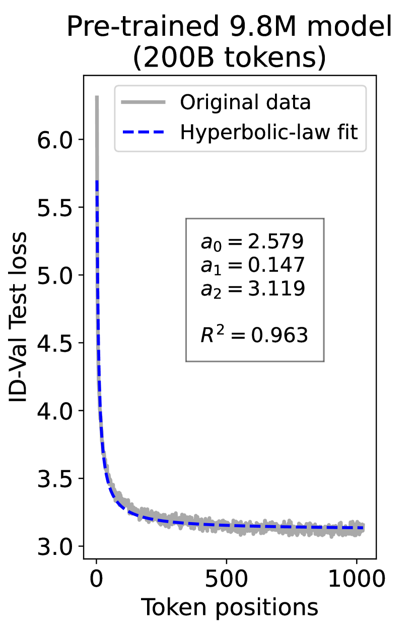
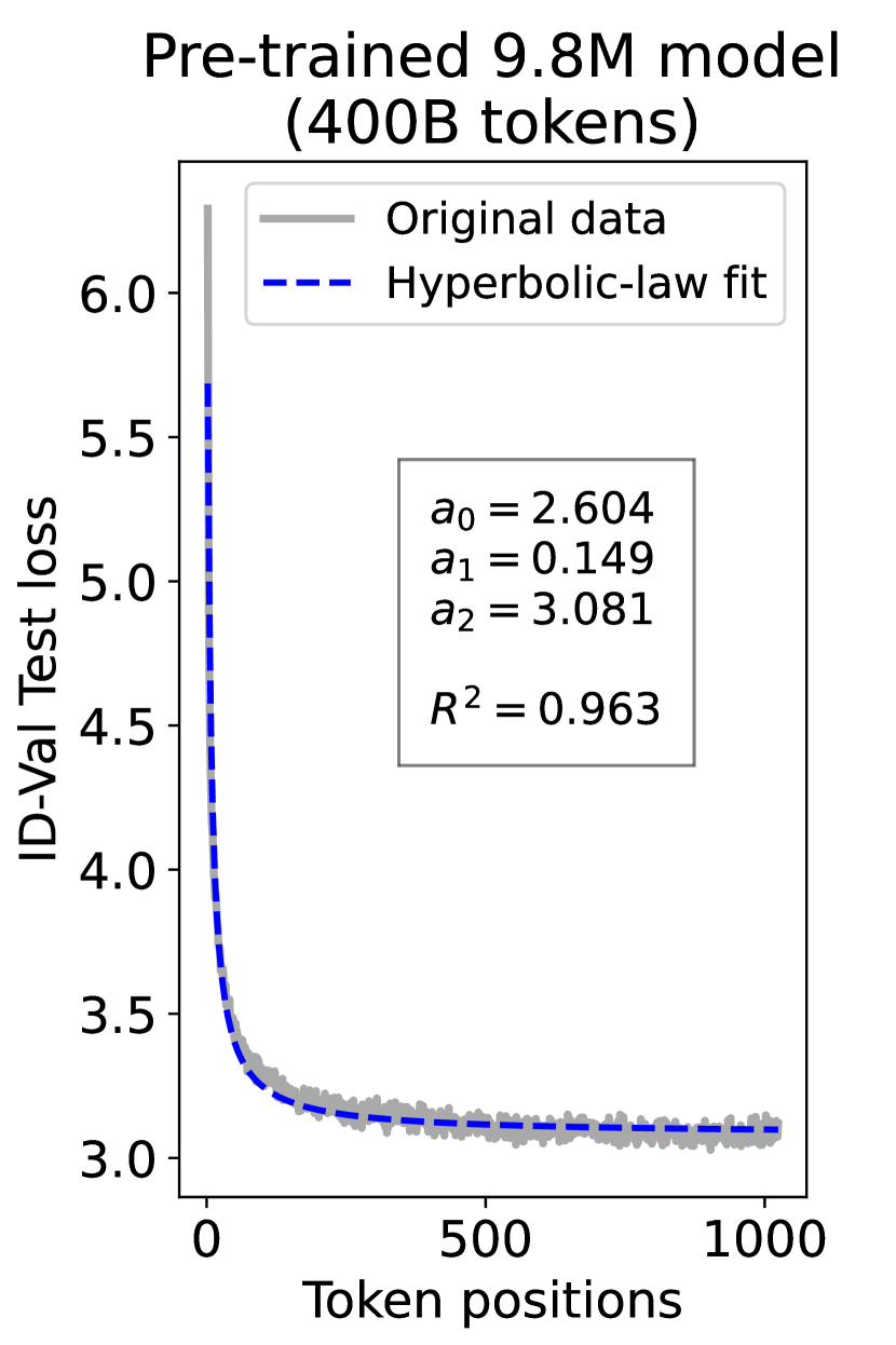
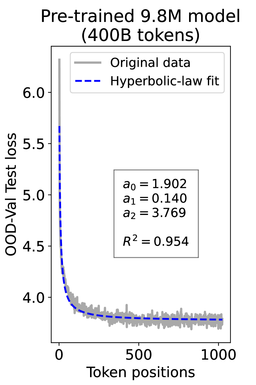
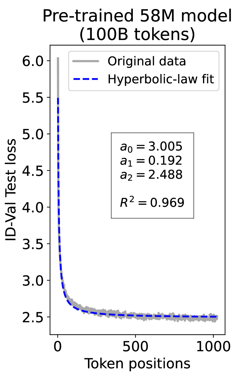
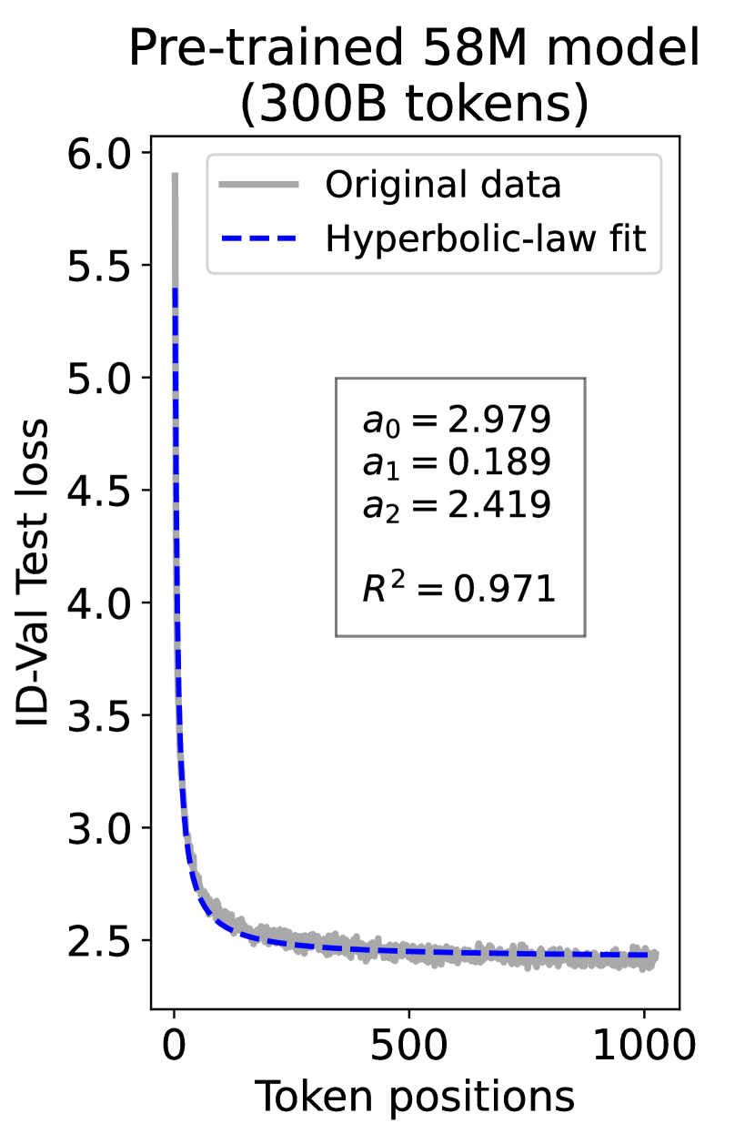
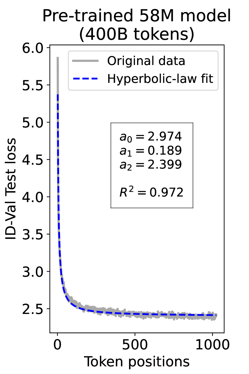
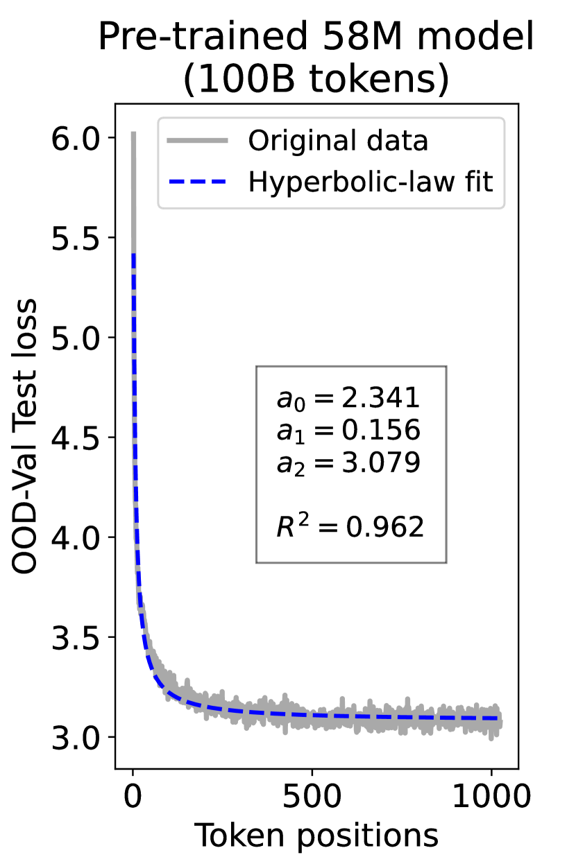
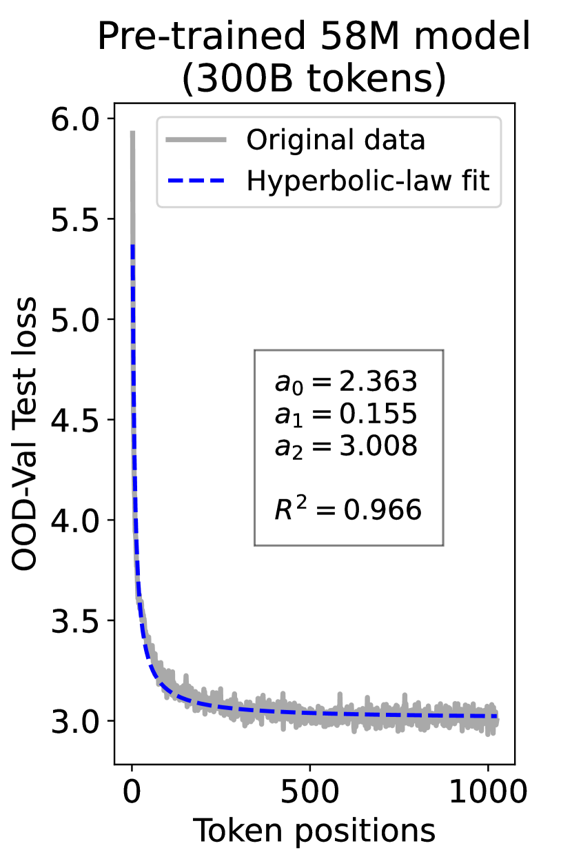
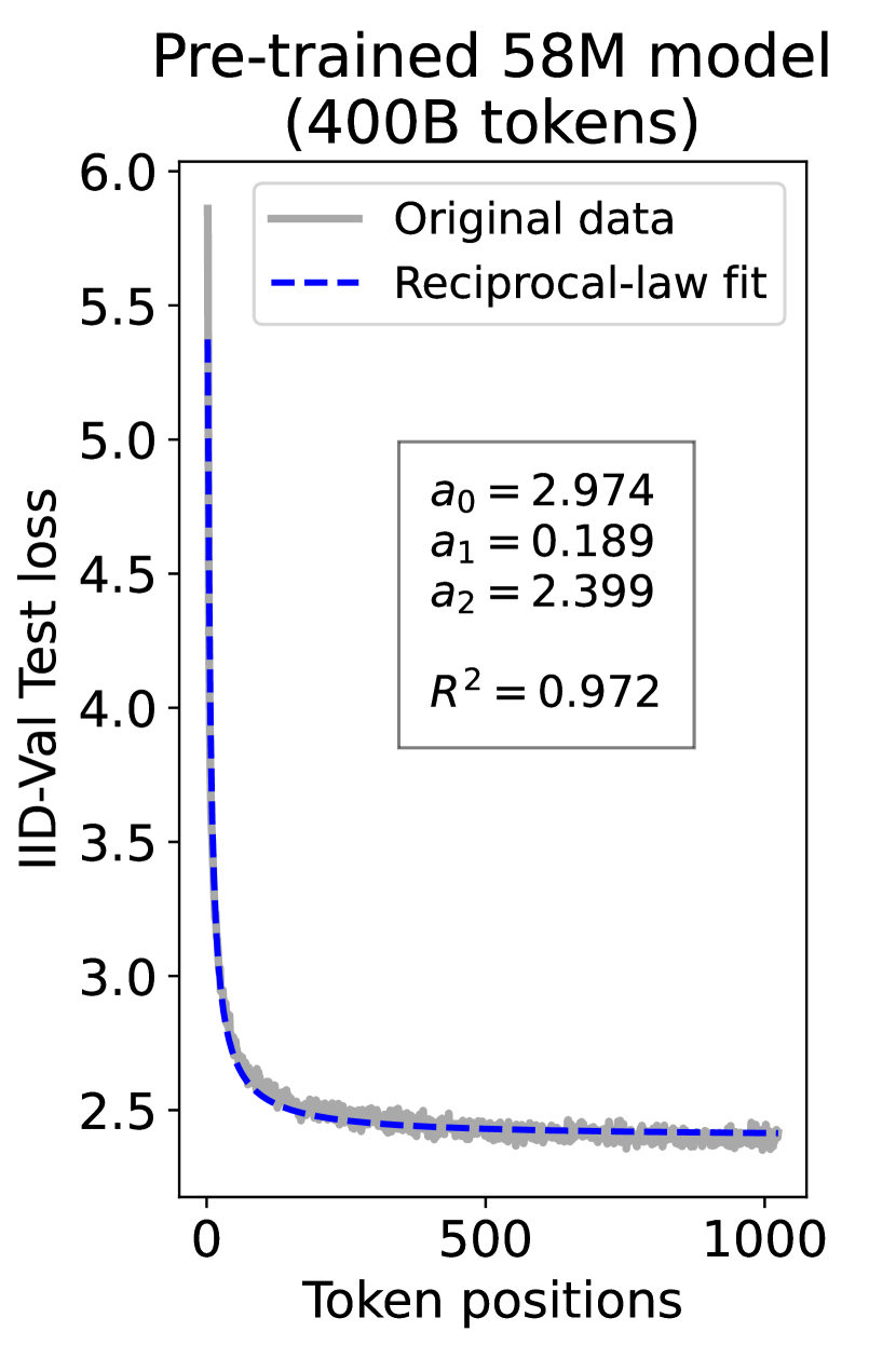
since has a longer context than . To illustrate this pattern, we plot the results of test loss for tokens in different positions, as validated on our ID-Val, using both our 9.8M and 58M models after training for 100B, 200B, 300B, and 400B tokens. We show the results for 400B tokens and leave the rest in the Appendix. As shown in Fig. 1, both models, although varying in scales, follow the same pattern that test loss for tokens with shorter context is commonly higher than that for tokens with longer context. For both models, the loss values for tokens near the end of the sequence seem to converge at a certain value. We find that this trend can be well fit with a hyperbolic relation:
| (5) |
where is the loss on token position , and , , and are fitting parameters solved by non-linear least squares. The fit for data from our 9.8M and 58M model are presented in Fig. 1. By applying this fit to test loss results of all checkpoints across the training phase, we find that over 99% of them can be fit with such hyperbolic relation with , well demonstrating its generality. We term this phenomenon as the dynamic hyperbolic-law. See appendix C for more insights.
We also tested Kaplan’s power-law Kaplan et al. (2020) and other functions that conform to Eq. 4 to fit the curve, but the results are suboptimal. For example, using the power-law yields for over 95% checkpoints. The conclusion still holds on the OOD-Val and on larger-scale models. See detailed results in appendix E.

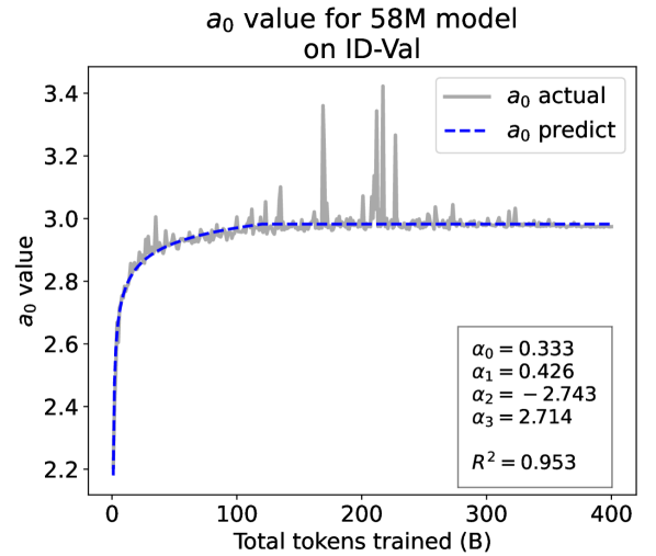
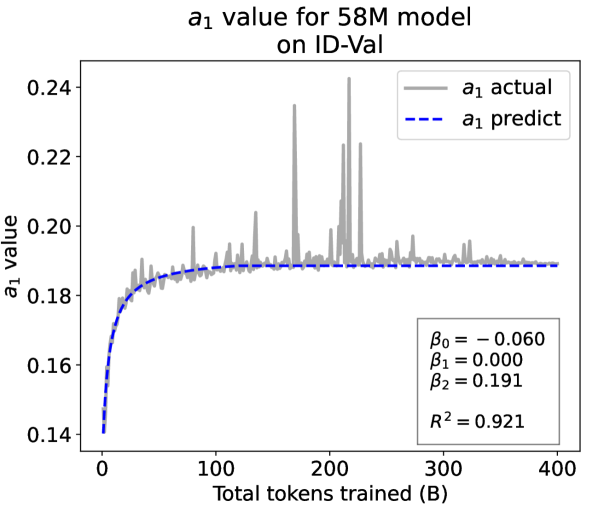

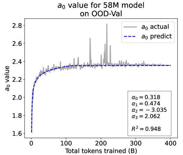
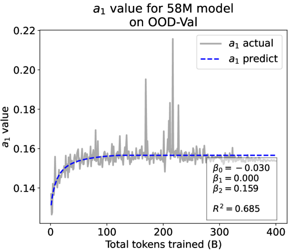
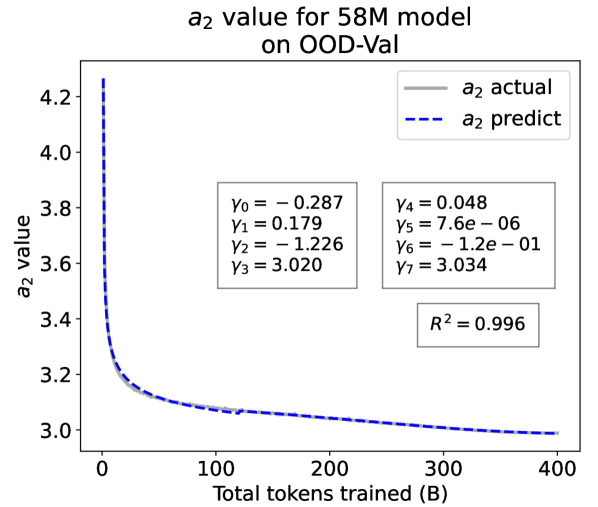
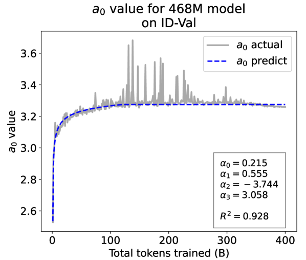
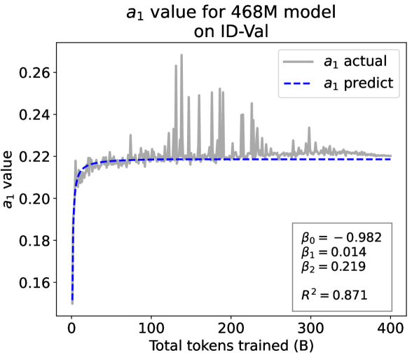
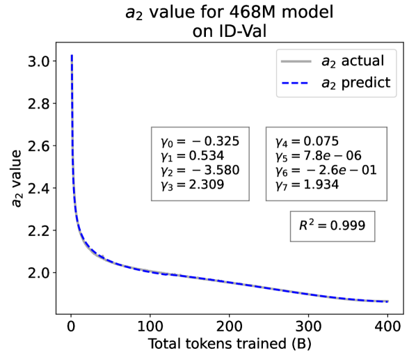
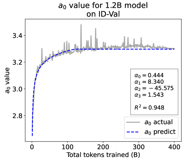
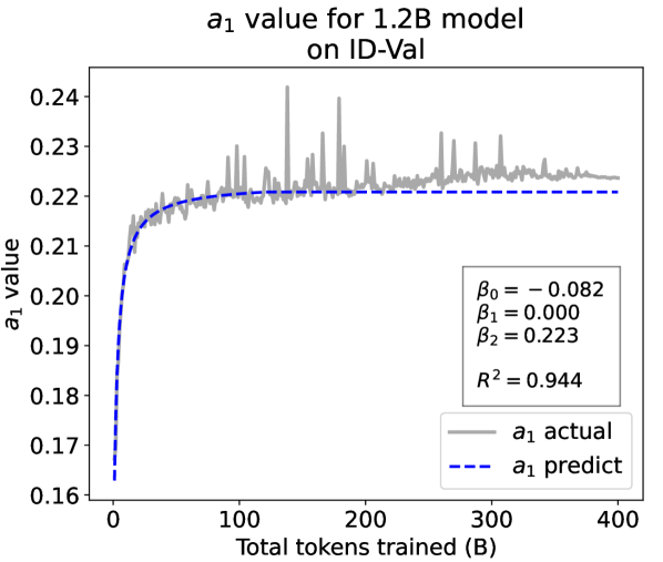
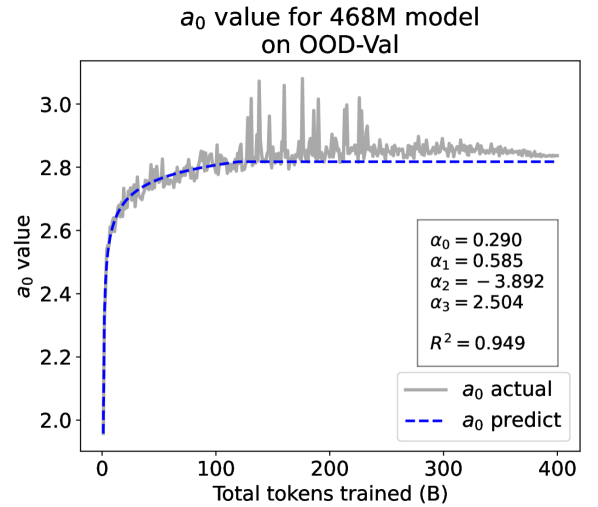
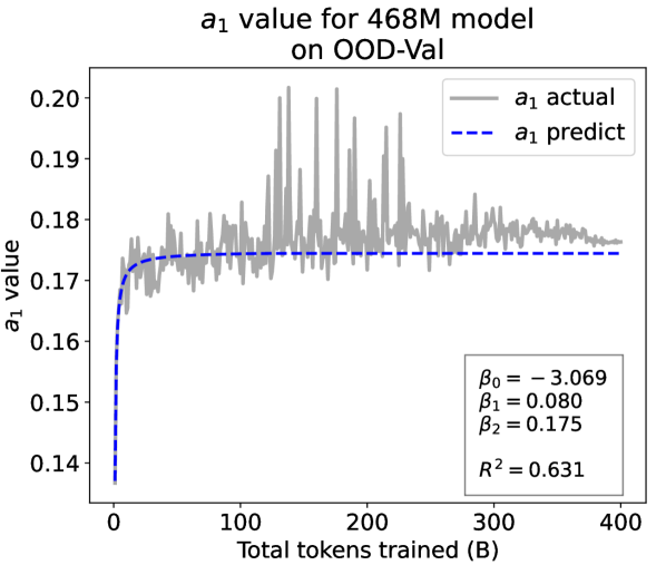
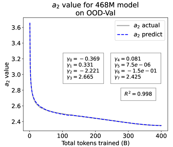
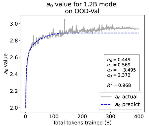
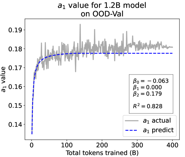
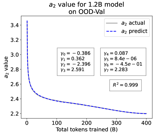
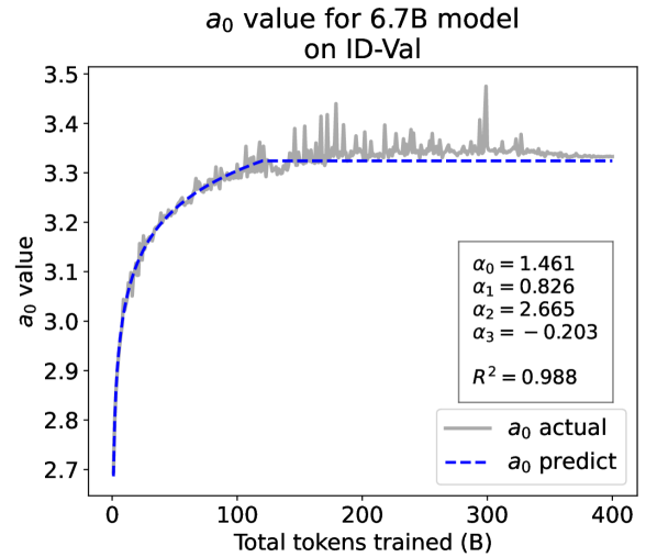
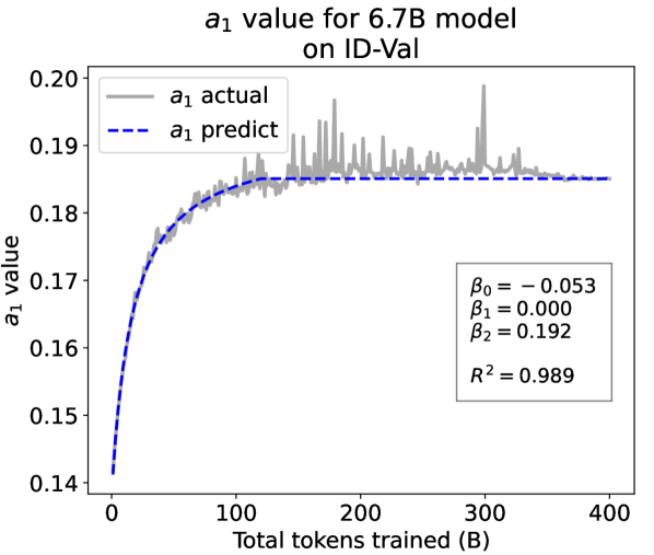
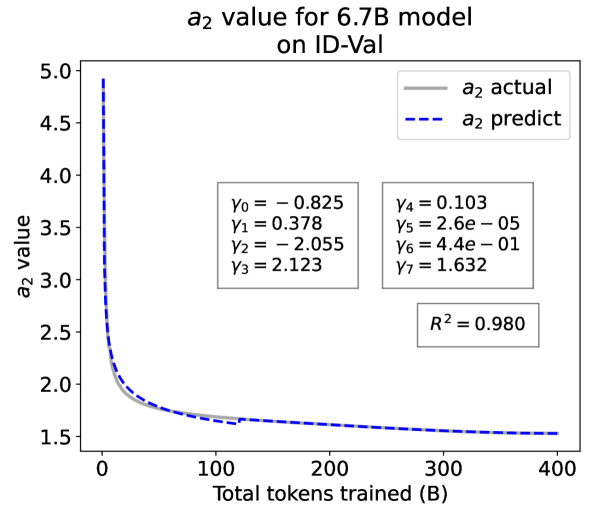
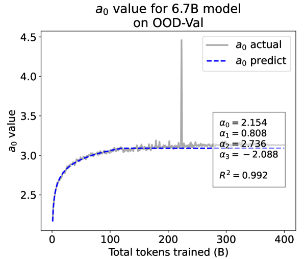
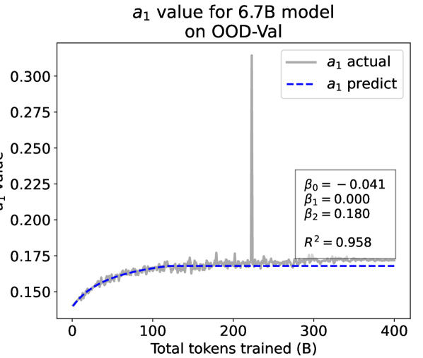
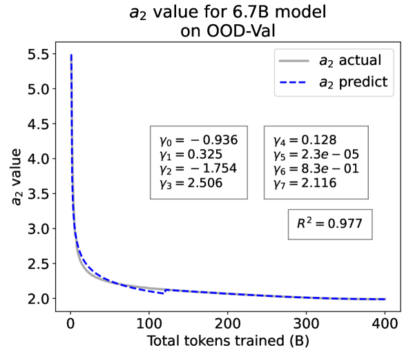
From the Dynamic Hyperbolic-law to the Overall Temporal Pattern. In the dynamic hyperbolic-law, is the converging factor denoting the converged value of loss on each tail token as context length increases. denotes the loss gap between the first token and the last token, and is the scaling factor along sequence length. To analyze how the derived values of , , and vary as training steps increase, we collect the derived value tuples of for all evaluated small model checkpoints during pretraining: , where is the number of trained tokens at the -th checkpoint, and is the total number of tokens used for pretraining. Then we plot the collected values on ID-Val w.r.t. the number of tokens trained (denoted as ) for the 58M model in Fig. 2. It can be seen that the evolution of , , and presents an evident pattern that can be fit by common functions. Therefore, it is possible for us to firstly fit the temporal evolution of , , and , and then fill them into Eq. 5 to depict the temporal evolution of the overall test loss.
First, for and , we use a series of common functions to fit their temporal evolution, and eventually choose the following functions that yield the lowest fitting errors:
| (6) | ||||
where the and fitting parameters are solved by non-linear least squares. Observed from the original data in Fig. 2, we find that the value of and generally converges after a period of training, but suffer from fluctuations after converging due to the uncertainty of the first prediction position in a sequence, which has no previous context to make prediction. To mitigate the fluctuations, we define a separation point :
| (7) |
And we manually stabilize and after :
| (8) |
Here we empirically set .
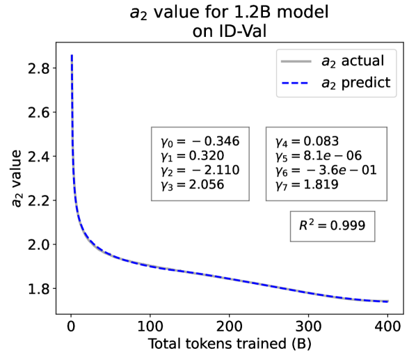
For parameter , we observe that is also a separation point as it marks the shift of its decreasing pattern. Before , we apply the same function form of the loss gap factor as in Eq. 6. After , we find that its temporal pattern holds strong correlations with the cosine learning rate scheduler, and in turn apply a cosine relation. Similar to Eq. 6, we search the common functions and choose the best fitting function among them for :
| (9) |
where are fitting parameters solved by non-linear least squares. Interestingly, from the fit for , we find that , indicating that the training schedule resembles half of a cosine period, consistent with the cosine scheduler. It further validates our speculation that has a strong correlation with the cosine learning rate decay.
We plot the fit of , , and in Fig. 2. Our fit captures the primary patterns of parameter evolution and ignores the insignificant fluctuations. The conclusion holds on the OOD-Val, and for larger models and models with other structures. See detailed results in appendices E and F.
After acquiring , , and , we could in turn measure the pattern of the total test loss by averaging the loss on each token:
| (10) |
As listed in Tab. 2, the fit for all ground-truth test losses during the whole training process achieves across different settings, demonstrating the validity of our temporal scaling law. Following Gao et al. (2021), We also validate the fitting results on the LAMBADA Paperno et al. (2016) and the WikiText Merity et al. (2017) datasets, both achieving . See appendix E for detailed results.
Summary. Overall, we summarize our temporal scaling law as follows:
-
•
For LLM pretraining, in each training step, the loss for tokens in different positions follows a dynamic hyperbolic-law, in which the values of parameters will change as training steps increase.
-
•
The temporal patterns (i.e., values at different training steps) of dynamic hyperbolic-law parameters (i.e., , , and ) can be captured individually with their corresponding coefficients (i.e., , , and ) in the fitting functions of fixed mathematical forms.
-
•
The temporal pattern of the overall test loss is derived by averaging losses at all token positions acquired by the dynamic hyperbolic-law, i.e., filling Eq. (6-9) into Eq. (10).
2.4 Test Loss Prediction
The primary value of scaling laws lies in their capability of predicting training outcomes Kaplan et al. (2020). From the temporal perspective, accurate predictions of the upcoming training periods can assist in a direct selection of hyperparameters based on the target LLM’s performance, early stopping, etc. In this section, we derive practical methods from our temporal scaling law to accurately predict the overall loss in the upcoming training periods, using data from an early training period to derive parameters of the temporal scaling law, during which only tokens are trained.
To predict the overall loss, we first predict the temporal trajectory of , , and . We could fit for and with the functions in Eq. 6:
| (11) | ||||
where and are fit using all collected with non-linear least squares. Following Eq. 7, we could estimate the separation point as . Based on the relationship of and , the test loss is predicted as:
Situation #1 (In most occasions): , i.e., in an early training stage where the separate point is not reached yet. For and , we apply the fit Eq. 11 for . For , we first fit the first segment in Eq. 9:
| (12) |
where are fit using non-linear least squares. Due to the absence of test loss data for , we could not acquire the value for , , and at that period directly. To estimate the patterns after the separation point, we propose general boundary conditions for estimation:
| (13) | ||||
According to the definition in Eq. 7, we simply stabilize the values for and as and correspondingly for , fulfilling the derivative condition in Eq. 13 approximately. For at , to eliminate the number of unknown variables, we directly adopt the discovery from fitting Eq. 9 that resembles half of a cosine period, and directly set . We set , where is the number of tokens used for warmup training, to ensure that marks the start point of a cosine period. We in turn solve for the rest parameters and in the following function based on Eq. 13:
| (14) |
Situation #2 (Otherwise): , i.e., in a middle stage where the separate point is already reached: Apart from steps in Situation #1, we additionally calibrate and with the data by estimating and :
| (15) |
After acquiring the complete estimations of , , and , we could calculate the test loss prediction for each training step with Eq. 10.
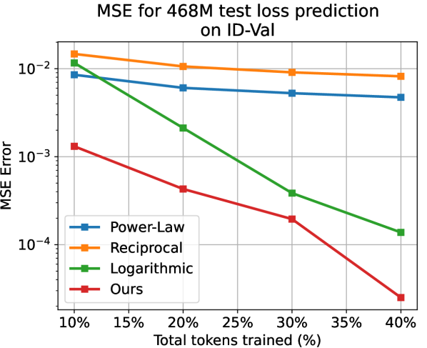
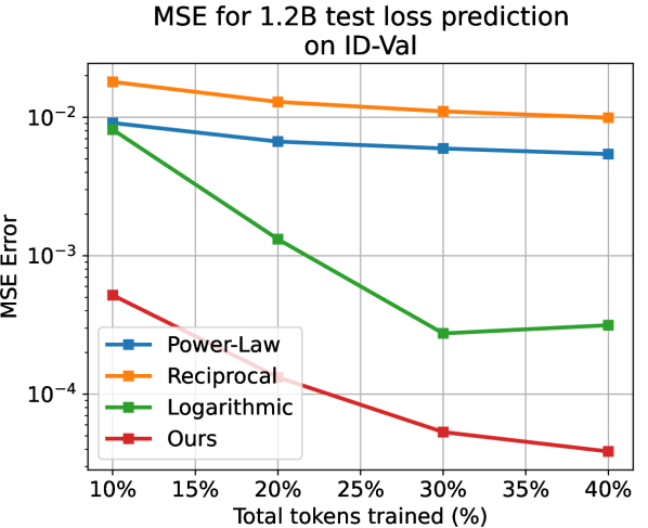
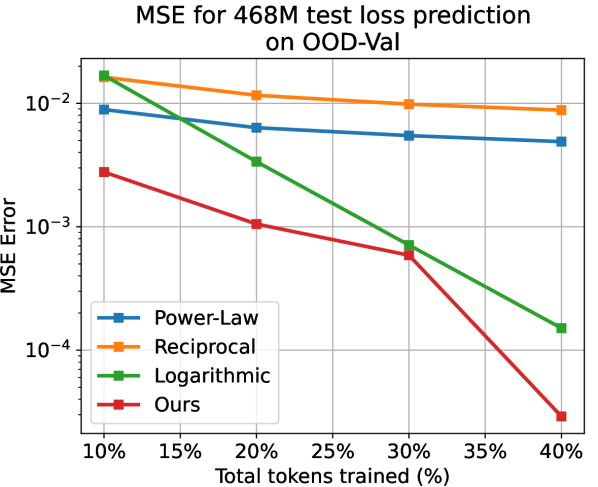
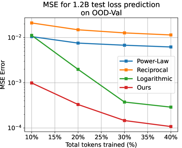
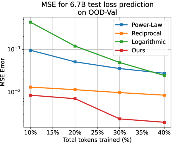
Experiments. Predicting test losses in upcoming training periods is a time series modeling problem. Following standard practice Wu et al. (2021); Liu et al. (2022), we choose MSE for evaluation:
| (16) |
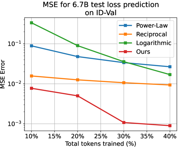
Apart from the power-law, we also choose the reciprocal () and the logarithmic () relations as baselines that model the test loss as a whole. We predict the subsequent test loss after deriving parameters of the temporal scaling law from, respectively, 10%, 20%, 30%, and 40% of the training process. Note that here we apply the larger models with 468M, 1.2B, and 6.7B parameters for validation. As shown in LABEL:{fig:fit_exp_result}, on different model scales and proportions of training, while the baselines hardly generate reliable results, our method always yields accurate results with . Our method yields far better as well. For example, when using 10% data for 1.2B model on ID-Val, our method yields , while the power-law, reciprocal, and logarithmic baselines yield , correspondingly. Those prediction results provide strong evidence for the reliability of our temporal scaling law. The conclusion holds on the OOD-Val. See appendix G for detailed results.
| BoolQ | HellaSwag | OpenBookQA | PIQA | SIQA | StoryCloze | Winogrande | ||
|---|---|---|---|---|---|---|---|---|
| 468M | Small Model / 10B Test Loss | 58.70 | 45.38 | 31.25 | 68.60 | 43.39 | 64.78 | 54.93 |
| Our pipeline | 57.07 | 45.98 | 33.68 | 69.36 | 44.01 | 64.88 | 54.02 | |
| 1.2B | Small Model / 10B Test Loss | 56.25 | 54.13 | 34.25 | 72.20 | 42.11 | 69.05 | 59.83 |
| Our pipeline | 58.70 | 54.51 | 34.90 | 72.36 | 46.73 | 69.11 | 60.32 |
| ID-Val | OOD-Val | ||
|---|---|---|---|
| 468M | Small Model / 10B Test Loss | 8.65 | 11.92 |
| Our pipeline | 8.58 | 11.77 | |
| 1.2B | Small Model / 10B Test Loss | 7.55 | 10.29 |
| Our pipeline | 7.50 | 10.17 |
3 Use Case #1 of Temporal Scaling Law: Hyperparameter Selection
Our temporal scaling law can be applied to enable a direct hyperparameter selection for LLMs. With our temporal scaling law, for hyperparameters that are completely un-transferrable such as the weight decay Yang et al. (2022), it is applicable to directly search them on the target large model from a candidate pool. As for hyperparameters that are "partially transferrable", e.g., data mixtures, small proxy models can help to identify a smaller range of effective candidates for the target large model, though not necessarily optimal. In such cases, our method is compatible with existing small-model-to-large-model hyperparameter searching methods, and here we could use a retrieval-rerank pipeline to achieve more precise results.
For example, data mixture proportions greatly affect the performance of LLMs Touvron et al. (2023a, b); Xie et al. (2023). Due to the huge computation cost of training with multiple data proportions directly on target LLMs, prior art simply applies the proportion values tuned on a much smaller model Xie et al. (2023). Using the temporal scaling law, we could accurately predict the final performance (in terms of test losses on validation sets) of different data proportions without completing the extensive pretraining.
Specifically, to select the best data mixture proportion for training a larger 468M/1.2B model, in the retrieval stage, following the prior art Xie et al. (2023), we use a small-scale model to locate a group of data mixture proportion candidates. In the rerank stage, we train all located data proportions on the target LLM for acceptable training tokens, and locate the best one by predicting their final losses with our temporal scaling law.
Experiment Setup. In the retrieval stage, we conduct a grid search on a 58M model and locate the Top-5 candidates. In the rerank stage, we train each candidate for 10B tokens before making the test loss prediction with Eq.11-14 on validation datasets. To validate the data mixture choices by temporal scaling law on the target 468M/1.2B models, we (1) primarily use the perplexity metric on the ID-Val and the OOD-Val, and also (2) follow Touvron et al. (2023a); Rae et al. (2021) and employ 7 popular common sense reasoning benchmarks, including BoolQ Clark et al. (2019), HellaSwag Zellers et al. (2019), OpenBookQA Mihaylov et al. (2018), PIQA Bisk et al. (2020), SIQA Sap et al. (2019), StoryCloze Mostafazadeh et al. (2016), and Winogrande Sakaguchi et al. (2021) for evaluating the final fully trained models. See the appendix H for more experimental details.
Experiment Result. We compare the data mixture proportion selected by our retrieval-rerank pipeline with the following baselines: (1) the Top-1 selected directly on the much smaller model and (2) the Top-1 selected by comparing the real test losses on ID-Val and OOD-Val validation sets after training 10B tokens on 468M/1.2B model. We find that both (1) and (2) make the same choice from the Top-5 candidates, and our pipeline locates a different choice from them. As shown in Tab. 4, our choice achieves lower perplexity across all settings after completing pretraining (i.e., 400B tokens). Additionally, as shown in Tab. 3, our choice yields superior benchmark performance in 12 of 14 metrics. Consequently, our approach of directly selecting hyperparameters on the target LLM is more effective and incurs an acceptable cost, which does not necessitates fully training the model.
4 Use Case #2 of Temporal Scaling Law: Revisit the Training Strategy
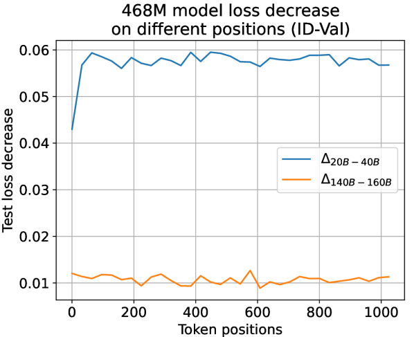
The temporal scaling law has afforded the possibility to study LLM pretraining in a finer granularity. As noted in Sec. 2.3, tokens on different positions possess a fundamental bias in learning difficulty. Specifically, head tokens are generally harder to predict than tail tokens. However, as suggested by Eqs. 6 and 8, and remain constant after the separation point. Therefore, for :
| (17) |
which is unrelated to token position , suggesting that LLMs learn equally on different token positions. To validate this observation, we trace the actual loss decrease observed during training along different token positions. It is observed that in a later training stage where the separation point conditions in Eq. 7 are already fulfilled, test loss decrease among all token positions tends to be uniform across all settings (see Fig. 11 for results). Such a consistency between theoretical prediction and experimental observation strongly validates the reasonableness and effectiveness of our temporal scaling law. Experiments also show that simply averaging losses on all token positions is an effective strategy for training LLMs. Refer to appendix I for more experimental settings and results.
5 Conclusion
Our research introduces the novel concept of Temporal Scaling Law for Large Language Models (LLMs), studying how the loss of an LLM evolves as the training steps scale up. We analyze the loss patterns on different token positions and discover that these patterns conform to a dynamic hyperbolic-law. By studying the temporal evolution of parameters of the dynamic hyperbolic-law, we could properly fit and precisely predict the evolution of the LLM’s test loss, marking a significant improvement over baseline methods. Such capability is crucial for numerous possible applications, like better hyperparameter selection directly on target LLM and deeper understanding pretraining dynamics of LLM, etc.
Limitations.
Our work termed Temporal Scaling Law, pioneers the modeling of LLM pre-training from a temporal perspective. Although our temporal scaling law exhibits significant potential for both LLM research and application, limitations still exist. Our research primarily focuses on the pre-training stage. The temporal patterns in other scenarios, such as transfer learning, are not covered. We leave further investigations of the above topics to our future research.
References
- Aghajanyan et al. (2023) Armen Aghajanyan, Lili Yu, Alexis Conneau, Wei-Ning Hsu, Karen Hambardzumyan, Susan Zhang, Stephen Roller, Naman Goyal, Omer Levy, and Luke Zettlemoyer. 2023. Scaling laws for generative mixed-modal language models. In International Conference on Machine Learning, ICML 2023, 23-29 July 2023, Honolulu, Hawaii, USA, volume 202 of Proceedings of Machine Learning Research, pages 265–279. PMLR.
- Andonian et al. (2023) Alex Andonian, Quentin Anthony, Stella Biderman, Sid Black, Preetham Gali, Leo Gao, Eric Hallahan, Josh Levy-Kramer, Connor Leahy, Lucas Nestler, Kip Parker, Michael Pieler, Jason Phang, Shivanshu Purohit, Hailey Schoelkopf, Dashiell Stander, Tri Songz, Curt Tigges, Benjamin Thérien, and 2 others. 2023. GPT-NeoX: Large Scale Autoregressive Language Modeling in PyTorch.
- Biderman et al. (2023) Stella Biderman, Hailey Schoelkopf, Quentin Gregory Anthony, Herbie Bradley, and Kyle O’Brien et al. 2023. Pythia: A suite for analyzing large language models across training and scaling. In International Conference on Machine Learning, ICML 2023, 23-29 July 2023, Honolulu, Hawaii, USA, volume 202 of Proceedings of Machine Learning Research, pages 2397–2430. PMLR.
- Bisk et al. (2020) Yonatan Bisk, Rowan Zellers, Ronan Le Bras, Jianfeng Gao, and Yejin Choi. 2020. PIQA: reasoning about physical commonsense in natural language. In The Thirty-Fourth AAAI Conference on Artificial Intelligence, AAAI 2020, The Thirty-Second Innovative Applications of Artificial Intelligence Conference, IAAI 2020, The Tenth AAAI Symposium on Educational Advances in Artificial Intelligence, EAAI 2020, New York, NY, USA, February 7-12, 2020, pages 7432–7439. AAAI Press.
- Brown et al. (2020) Tom B. Brown, Benjamin Mann, Nick Ryder, Melanie Subbiah, Jared Kaplan, and Prafulla Dhariwal et al. 2020. Language models are few-shot learners. In Advances in Neural Information Processing Systems 33: Annual Conference on Neural Information Processing Systems 2020, NeurIPS 2020, December 6-12, 2020, virtual.
- Cheng et al. (2014) C.-L. Cheng, Shalabh, and G. Garg. 2014. Coefficient of determination for multiple measurement error models. Journal of Multivariate Analysis, 126:137–152.
- Cherti et al. (2023) Mehdi Cherti, Romain Beaumont, Ross Wightman, Mitchell Wortsman, Gabriel Ilharco, Cade Gordon, Christoph Schuhmann, Ludwig Schmidt, and Jenia Jitsev. 2023. Reproducible scaling laws for contrastive language-image learning. In IEEE/CVF Conference on Computer Vision and Pattern Recognition, CVPR 2023, Vancouver, BC, Canada, June 17-24, 2023, pages 2818–2829. IEEE.
- Chowdhery et al. (2023) Aakanksha Chowdhery, Sharan Narang, Jacob Devlin, Maarten Bosma, Gaurav Mishra, Adam Roberts, and Paul Barham et al. 2023. Palm: Scaling language modeling with pathways. J. Mach. Learn. Res., 24:240:1–240:113.
- Clark et al. (2019) Christopher Clark, Kenton Lee, Ming-Wei Chang, Tom Kwiatkowski, Michael Collins, and Kristina Toutanova. 2019. Boolq: Exploring the surprising difficulty of natural yes/no questions. In Proceedings of the 2019 Conference of the North American Chapter of the Association for Computational Linguistics: Human Language Technologies, NAACL-HLT 2019, Minneapolis, MN, USA, June 2-7, 2019, Volume 1 (Long and Short Papers), pages 2924–2936. Association for Computational Linguistics.
- Devlin et al. (2019) Jacob Devlin, Ming-Wei Chang, Kenton Lee, and Kristina Toutanova. 2019. BERT: pre-training of deep bidirectional transformers for language understanding. In Proceedings of the 2019 Conference of the North American Chapter of the Association for Computational Linguistics: Human Language Technologies, NAACL-HLT 2019, Minneapolis, MN, USA, June 2-7, 2019, Volume 1 (Long and Short Papers), pages 4171–4186. Association for Computational Linguistics.
- Fedus et al. (2022) William Fedus, Barret Zoph, and Noam Shazeer. 2022. Switch transformers: Scaling to trillion parameter models with simple and efficient sparsity. J. Mach. Learn. Res., 23:120:1–120:39.
- Gao et al. (2021) Leo Gao, Stella Biderman, Sid Black, Laurence Golding, Travis Hoppe, Charles Foster, Jason Phang, Horace He, Anish Thite, Noa Nabeshima, Shawn Presser, and Connor Leahy. 2021. The pile: An 800gb dataset of diverse text for language modeling. CoRR, abs/2101.00027.
- Gao et al. (2023) Leo Gao, Jonathan Tow, Baber Abbasi, Stella Biderman, Sid Black, Anthony DiPofi, Charles Foster, Laurence Golding, Jeffrey Hsu, Alain Le Noac’h, Haonan Li, Kyle McDonell, Niklas Muennighoff, Chris Ociepa, Jason Phang, Laria Reynolds, Hailey Schoelkopf, Aviya Skowron, Lintang Sutawika, and 5 others. 2023. A framework for few-shot language model evaluation.
- Henighan et al. (2020) Tom Henighan, Jared Kaplan, Mor Katz, Mark Chen, Christopher Hesse, and Jacob Jackson et al. 2020. Scaling laws for autoregressive generative modeling. CoRR, abs/2010.14701.
- Hernandez et al. (2021) Danny Hernandez, Jared Kaplan, Tom Henighan, and Sam McCandlish. 2021. Scaling laws for transfer. CoRR, abs/2102.01293.
- Hoffmann et al. (2022) Jordan Hoffmann, Sebastian Borgeaud, Arthur Mensch, Elena Buchatskaya, Trevor Cai, Eliza Rutherford, Diego de Las Casas, Lisa Anne Hendricks, Johannes Welbl, Aidan Clark, Tom Hennigan, Eric Noland, Katie Millican, George van den Driessche, Bogdan Damoc, Aurelia Guy, Simon Osindero, Karen Simonyan, Erich Elsen, and 3 others. 2022. Training compute-optimal large language models. CoRR, abs/2203.15556.
- Huang et al. (2024) Quzhe Huang, Zhenwei An, Nan Zhuang, Mingxu Tao, Chen Zhang, Yang Jin, Kun Xu, Liwei Chen, Songfang Huang, and Yansong Feng. 2024. Harder tasks need more experts: Dynamic routing in moe models. arXiv preprint arXiv:2403.07652.
- Isik et al. (2024) Berivan Isik, Natalia Ponomareva, Hussein Hazimeh, Dimitris Paparas, Sergei Vassilvitskii, and Sanmi Koyejo. 2024. Scaling laws for downstream task performance of large language models. CoRR, abs/2402.04177.
- Kaplan et al. (2020) Jared Kaplan, Sam McCandlish, Tom Henighan, Tom B. Brown, Benjamin Chess, Rewon Child, Scott Gray, Alec Radford, Jeffrey Wu, and Dario Amodei. 2020. Scaling laws for neural language models. CoRR, abs/2001.08361.
- Liu et al. (2022) Yong Liu, Haixu Wu, Jianmin Wang, and Mingsheng Long. 2022. Non-stationary transformers: Exploring the stationarity in time series forecasting. In Advances in Neural Information Processing Systems 35: Annual Conference on Neural Information Processing Systems 2022, NeurIPS 2022, New Orleans, LA, USA, November 28 - December 9, 2022.
- Loshchilov and Hutter (2017) Ilya Loshchilov and Frank Hutter. 2017. SGDR: stochastic gradient descent with warm restarts. In 5th International Conference on Learning Representations, ICLR 2017, Toulon, France, April 24-26, 2017, Conference Track Proceedings. OpenReview.net.
- Loshchilov and Hutter (2019) Ilya Loshchilov and Frank Hutter. 2019. Decoupled weight decay regularization. In 7th International Conference on Learning Representations, ICLR 2019, New Orleans, LA, USA, May 6-9, 2019. OpenReview.net.
- Merity et al. (2017) Stephen Merity, Caiming Xiong, James Bradbury, and Richard Socher. 2017. Pointer sentinel mixture models. In 5th International Conference on Learning Representations, ICLR 2017, Toulon, France, April 24-26, 2017, Conference Track Proceedings. OpenReview.net.
- Mihaylov et al. (2018) Todor Mihaylov, Peter Clark, Tushar Khot, and Ashish Sabharwal. 2018. Can a suit of armor conduct electricity? A new dataset for open book question answering. In Proceedings of the 2018 Conference on Empirical Methods in Natural Language Processing, Brussels, Belgium, October 31 - November 4, 2018, pages 2381–2391. Association for Computational Linguistics.
- Mostafazadeh et al. (2016) Nasrin Mostafazadeh, Nathanael Chambers, Xiaodong He, Devi Parikh, Dhruv Batra, Lucy Vanderwende, Pushmeet Kohli, and James F. Allen. 2016. A corpus and evaluation framework for deeper understanding of commonsense stories. CoRR, abs/1604.01696.
- OpenAI (2023) OpenAI. 2023. GPT-4 technical report. CoRR, abs/2303.08774.
- Paperno et al. (2016) Denis Paperno, Germán Kruszewski, Angeliki Lazaridou, Quan Ngoc Pham, Raffaella Bernardi, Sandro Pezzelle, Marco Baroni, Gemma Boleda, and Raquel Fernández. 2016. The LAMBADA dataset: Word prediction requiring a broad discourse context. In Proceedings of the 54th Annual Meeting of the Association for Computational Linguistics, ACL 2016, August 7-12, 2016, Berlin, Germany, Volume 1: Long Papers. The Association for Computer Linguistics.
- Que et al. (2024) Haoran Que, Jiaheng Liu, Ge Zhang, Chenchen Zhang, Xingwei Qu, Yinghao Ma, Feiyu Duan, Zhiqi Bai, Jiakai Wang, Yuanxing Zhang, Xu Tan, Jie Fu, Wenbo Su, Jiamang Wang, Lin Qu, and Bo Zheng. 2024. D-CPT law: Domain-specific continual pre-training scaling law for large language models. CoRR, abs/2406.01375.
- Radford et al. (2018) Alec Radford, Karthik Narasimhan, Tim Salimans, Ilya Sutskever, and 1 others. 2018. Improving language understanding by generative pre-training.
- Radford et al. (2019) Alec Radford, Jeffrey Wu, Rewon Child, David Luan, Dario Amodei, Ilya Sutskever, and 1 others. 2019. Language models are unsupervised multitask learners. OpenAI blog, 1(8):9.
- Rae et al. (2021) Jack W. Rae, Sebastian Borgeaud, Trevor Cai, Katie Millican, Jordan Hoffmann, H. Francis Song, and John Aslanides et al. 2021. Scaling language models: Methods, analysis & insights from training gopher. CoRR, abs/2112.11446.
- Raffel et al. (2020) Colin Raffel, Noam Shazeer, Adam Roberts, Katherine Lee, Sharan Narang, Michael Matena, Yanqi Zhou, Wei Li, and Peter J. Liu. 2020. Exploring the limits of transfer learning with a unified text-to-text transformer. J. Mach. Learn. Res., 21:140:1–140:67.
- Sakaguchi et al. (2021) Keisuke Sakaguchi, Ronan Le Bras, Chandra Bhagavatula, and Yejin Choi. 2021. Winogrande: an adversarial winograd schema challenge at scale. Commun. ACM, 64(9):99–106.
- Sap et al. (2019) Maarten Sap, Hannah Rashkin, Derek Chen, Ronan Le Bras, and Yejin Choi. 2019. Socialiqa: Commonsense reasoning about social interactions. CoRR, abs/1904.09728.
- Su et al. (2024a) Zhenpeng Su, Zijia Lin, Xue Bai, Xing Wu, Yizhe Xiong, Haoran Lian, Guangyuan Ma, Hui Chen, Guiguang Ding, Wei Zhou, and 1 others. 2024a. Maskmoe: Boosting token-level learning via routing mask in mixture-of-experts. arXiv preprint arXiv:2407.09816.
- Su et al. (2023) Zhenpeng Su, Xing Wu, Xue Bai, Zijia Lin, Hui Chen, Guiguang Ding, Wei Zhou, and Songlin Hu. 2023. Infoentropy loss to mitigate bias of learning difficulties for generative language models. CoRR, abs/2310.19531.
- Su et al. (2024b) Zhenpeng Su, Xing Wu, Zijia Lin, Yizhe Xiong, Minxuan Lv, Guangyuan Ma, Hui Chen, Songlin Hu, and Guiguang Ding. 2024b. Cartesianmoe: Boosting knowledge sharing among experts via cartesian product routing in mixture-of-experts. arXiv preprint arXiv:2410.16077.
- Touvron et al. (2023a) Hugo Touvron, Thibaut Lavril, Gautier Izacard, Xavier Martinet, Marie-Anne Lachaux, Timothée Lacroix, Baptiste Rozière, Naman Goyal, Eric Hambro, Faisal Azhar, Aurélien Rodriguez, Armand Joulin, Edouard Grave, and Guillaume Lample. 2023a. Llama: Open and efficient foundation language models. CoRR, abs/2302.13971.
- Touvron et al. (2023b) Hugo Touvron, Louis Martin, Kevin Stone, Peter Albert, Amjad Almahairi, and Yasmine Babaei et al. 2023b. Llama 2: Open foundation and fine-tuned chat models. CoRR, abs/2307.09288.
- Vaswani et al. (2017) Ashish Vaswani, Noam Shazeer, Niki Parmar, Jakob Uszkoreit, Llion Jones, Aidan N. Gomez, Lukasz Kaiser, and Illia Polosukhin. 2017. Attention is all you need. In Advances in Neural Information Processing Systems 30: Annual Conference on Neural Information Processing Systems 2017, December 4-9, 2017, Long Beach, CA, USA, pages 5998–6008.
- Wortsman et al. (2024) Mitchell Wortsman, Peter J. Liu, Lechao Xiao, Katie E. Everett, Alexander A. Alemi, Ben Adlam, John D. Co-Reyes, Izzeddin Gur, Abhishek Kumar, Roman Novak, Jeffrey Pennington, Jascha Sohl-Dickstein, Kelvin Xu, Jaehoon Lee, Justin Gilmer, and Simon Kornblith. 2024. Small-scale proxies for large-scale transformer training instabilities. In The Twelfth International Conference on Learning Representations, ICLR 2024, Vienna, Austria, May 7-11, 2024. OpenReview.net.
- Wu et al. (2021) Haixu Wu, Jiehui Xu, Jianmin Wang, and Mingsheng Long. 2021. Autoformer: Decomposition transformers with auto-correlation for long-term series forecasting. In Advances in Neural Information Processing Systems 34: Annual Conference on Neural Information Processing Systems 2021, NeurIPS 2021, December 6-14, 2021, virtual, pages 22419–22430.
- Xie et al. (2023) Sang Michael Xie, Hieu Pham, Xuanyi Dong, Nan Du, Hanxiao Liu, Yifeng Lu, Percy Liang, Quoc V. Le, Tengyu Ma, and Adams Wei Yu. 2023. Doremi: Optimizing data mixtures speeds up language model pretraining. CoRR, abs/2305.10429.
- Yang et al. (2022) Greg Yang, Edward J. Hu, Igor Babuschkin, Szymon Sidor, Xiaodong Liu, David Farhi, Nick Ryder, Jakub Pachocki, Weizhu Chen, and Jianfeng Gao. 2022. Tensor programs V: tuning large neural networks via zero-shot hyperparameter transfer. CoRR, abs/2203.03466.
- Ye et al. (2024) Jiasheng Ye, Peiju Liu, Tianxiang Sun, Yunhua Zhou, Jun Zhan, and Xipeng Qiu. 2024. Data mixing laws: Optimizing data mixtures by predicting language modeling performance. CoRR, abs/2403.16952.
- Zellers et al. (2019) Rowan Zellers, Ari Holtzman, Yonatan Bisk, Ali Farhadi, and Yejin Choi. 2019. Hellaswag: Can a machine really finish your sentence? In Proceedings of the 57th Conference of the Association for Computational Linguistics, ACL 2019, Florence, Italy, July 28- August 2, 2019, Volume 1: Long Papers, pages 4791–4800. Association for Computational Linguistics.
Appendix A Related Works
A.1 Large Language Models
Language models are statistical models designed to model the probabilistic correlation in natural language sequences Touvron et al. (2023a). The introduction of the Transformer architecture Vaswani et al. (2017) led to the development of large language models. GPT-3 Brown et al. (2020) marks the beginning of the LLM era, as decoder-based generative models are capable of completing various tasks via in-context learning. Further advancements in LLMs include PaLM Chowdhery et al. (2023), Pythia Biderman et al. (2023), LLaMA Touvron et al. (2023a), etc. Currently, GPT-4 OpenAI (2023) has pushed the boundaries of LLMs further in terms of scale and capability.
A.2 Scaling Laws for Language Models
The concept of scaling laws for language models was proposed by Kaplan et al. (2020). Their study revealed that the test loss for generative transformer models scales as a power-law with model size, dataset size, and the amount of computation used for training. Building upon that foundational study, further research has expanded the concept of scaling laws to diverse problem settings Hernandez et al. (2021) and model architectures Cherti et al. (2023); Aghajanyan et al. (2023). For instance, Hernandez et al. (2021) has investigated scaling laws for transfer learning. Cherti et al. (2023) and Aghajanyan et al. (2023) observed scaling laws for multi-modal model pertaining. Furthermore, some recent works discovered other patterns beside the power-law for different problem settings, such as continual pertaining Que et al. (2024), data mixtures Ye et al. (2024), and training instabilities Wortsman et al. (2024). These works follow a small-model-to-large-model perspective and predict the final performance of large models by fitting the final training results on smaller models. Recently, researchers have also investigated scaling laws in the context of transfer learning Isik et al. (2024), where model performance is influenced by both the size of the training dataset and the degree of downstream task alignment.
Despite previous advancements, a critical point that remains underexplored is the temporal trajectory of LLM performance throughout training. Previous works Kaplan et al. (2020) estimate that the final test loss after training individually with different dataset sizes follows a power-law. However, such a coarse-grained estimation is not accurate enough in portraying the test loss evolution during a single pretrain process. By studying the loss behavior on different token positions, we introduce the temporal scaling law, allowing for more precise tracking and prediction of LLM test loss during pretraining. Our temporal scaling law focuses on the test loss evolution in a single pretrain process, while prior scaling laws model the relations of final test loss and the computational budget (model size, dataset size, etc.).
| model size | dimension | intermediate | heads | layers | learning rate | scheduler | warmup | optimizer | batch size | seq length |
|---|---|---|---|---|---|---|---|---|---|---|
| 9.8M | 128 | 512 | 4 | 6 | cosine | steps | AdamW | 1024 | 1024 | |
| 58M | 512 | 2048 | 8 | 6 | cosine | steps | AdamW | 1024 | 1024 | |
| 468M | 1024 | 4096 | 16 | 24 | cosine | steps | AdamW | 1024 | 1024 | |
| 1.2B | 2048 | 8192 | 8 | 16 | cosine | steps | AdamW | 1024 | 1024 | |
| 6.7B | 4096 | 11008 | 32 | 32 | cosine | steps | AdamW | 2048 | 2048 |
| model name | dimension | intermediate | heads | layers | learning rate | scheduler | warmup | optimizer | batch size | seq length |
|---|---|---|---|---|---|---|---|---|---|---|
| 468M GPT-NeoX | 1024 | 4096 | 16 | 24 | cosine | steps | AdamW | 1024 | 1024 | |
| 1.4B MoE (act: 240M) | 768 | 3072 | 12 | 12 | cosine | steps | AdamW | 1024 | 1024 |
| Package | Version | Package | Version |
|---|---|---|---|
| PyTorch | 2.1.0 | transformers | 4.32.0 |
| deepspeed | 0.10.0 | tokenizers | 0.13.3 |
| flash-attn | 2.3.6 | lm-evaluation-harness | 0.3.0 |
| datasets | 2.14.3 |
Appendix B Further Experiment Details
In this section, we provide further details toward the experiment settings in the article.
License for Scientific Artifacts. The Pile Gao et al. (2021) is subject to the MIT license222https://arxiv.org/pdf/2201.07311. The C4 dataset Raffel et al. (2020) is licensed under Open Data Commons License Attribution family333https://huggingface.co/datasets/allenai/c4. The LAMBADA dataset Paperno et al. (2016) is licensed under Creative Commons Attribution 4.0 International license444https://huggingface.co/datasets/cimec/lambada. The Wikitext dataset Merity et al. (2017) is licensed under the Creative Commons Attribution 4.0 International licence555https://zenodo.org/records/2630551. The evaluation benchmarks Gao et al. (2023) are subject to the MIT license. All usages of scientific artifacts in this paper obey the corresponding licenses.
Hyperparameters of Models Used. We report the details of model hyperparameters and training hyperparameters in Tab. 5. Note that we use the 9.8M and the 58M models for illustrating our temporal scaling law. Meanwhile, we apply the predictions and further applications of our temporal scaling law to the larger 468M and the 1.2B models.
Parameters for Packages. We report the version numbers of used packages in Tab. 7.
Evaluation Pipeline. For all benchmark evaluations, we utilize the open-source LLM evaluation tool lm-evaluation-harness666https://github.com/EleutherAI/lm-evaluation-harness Gao et al. (2023), following Su et al. (2023); Biderman et al. (2023). For all numerical results, we report the average result tested on the last 5 checkpoints.
Appendix C Theoretical Insights for the Dynamic Hyperbolic Law
Following prior work on validating scaling laws Kaplan et al. (2020); Hoffmann et al. (2022), we conducted comprehensive experiments and empirically confirmed the effectiveness of the hyperbolic pattern in the main article. In the main article, the main functional forms that we have considered are the logarithmic function (), power-law (), log-log function (), and exponential function () (see Sec. 2.4 for the experimental comparisons with those functions). In addition, we provide a theoretical justification for selecting the hyperbolic function among candidate forms. Specifically, the loss with respect to token positions should approach a lower bound, since the cross-entropy loss has a minimum of zero. This constraint limits the valid choices to the power-law, exponential, and hyperbolic functions. We then analyze the simplified forms of the power-law and exponential functions: for the power-law, , , ; for the exponential, , , . It is straightforward to show that the exponential function decays faster than the power-law. Formally, for all valid parameters, there exists an such that for all . Given that real-world corpus data typically does not yield losses approaching zero, the exponential function is impractical. Lastly, we note that the hyperbolic function can be rewritten in a power-law-like form as . Since this formulation not only satisfies theoretical constraints but also yields better empirical performance, we adopt it as the underlying structure for modeling token position loss.
Appendix D Pipeline for Predicting Training Outcomes Using the Temporal Scaling Law
We provide the pipeline for predicting the training outcomes using the temporal scaling law in algorithm 1. Note that we use non-linear least squares to solve for all fitting parameters. Normally, the fitting would converge in steps, which takes <1 second on a CPU. We conduct a re-fit for and to mitigate the effect of fluctuations (as observed in Fig. 2 in the article).
Appendix E Complete Fitting Results
Due to the page limit, we omitted some fitting results when illustrating our proposed temporal scaling law. In this section, we will present those fitting figures in detail.
E.1 More Results of Dynamic Hyperbolic-Law
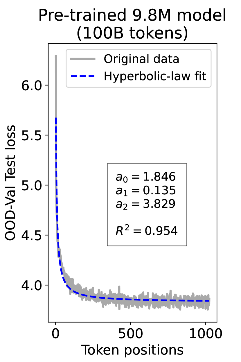
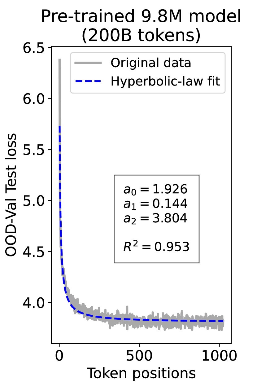
As a supplement to Figure 1 in Section 3.3 of the article, we provide fitting results of the dynamic hyperbolic-law for both the 9.8M and 58M models after training for 100B, 200B, 300B, and 400B tokens and on the OOD-Val in Fig. 6 and Fig. 7, respectively. Those results indicate that our dynamic hyperbolic-law consistently achieves accurate fitting results across model sizes and training steps.
E.2 More Results of Temporal Scaling Law
As a supplement to Figure 2 in Section 3.3 of the article, we provide the results on the OOD-Val in Fig. 8. We also provide fitting results on both the ID-Val and the OOD-Val for the larger 468M, 1.2B, and 6.7B model scales in Fig. 9 and Fig. 10. Across different settings on model scales and validation set distributions, our temporal scaling law is able to depict the general trend of parameter evolution and reduce the influence of fluctuations as much as possible.
| Model | LAMBADA | Wikitext |
|---|---|---|
| 9.8M | 0.9887 | 0.9809 |
| 58M | 0.9805 | 0.9899 |
| 468M | 0.9831 | 0.9920 |
| 1.2B | 0.9859 | 0.9930 |
| 6.7B | 0.9872 | 0.9927 |
| Strategy Name | Description |
|---|---|
| Default Practice | Average loss on all token positions. |
| Head Suppression | Weight loss on the foremost 10% tokens by 0.5x. |
| Body Suppression | Weight loss on the central 80% tokens by 0.5x. |
| Tail Suppression | Weight loss on the last 10% tokens by 0.5x. |
| Default Practice | Head | Body | Tail | |
|---|---|---|---|---|
| 468M | 8.62 | 8.62 | 8.66 | 8.63 |
| 1.2B | 7.52 | 7.52 | 7.56 | 7.53 |
E.3 Fitting Results on More Datasets
In the article, we have proposed the temporal scaling law to precisely fit the temporal evolution of test loss during LLM pretraining. To better demonstrate the validity of our temporal scaling law, we also validate the fitting results of the 9.8M and 58M models on the LAMBADA Paperno et al. (2016) and the WikiText Merity et al. (2017) datasets. Specifically, we use the validation and the test splits for the LAMBADA dataset, and use the wikitext-2-v1 domain for the WikiText dataset. The results are shown in Tab. 8. We also provide the fitting results for the larger 468M, 1.2B, and 6.7B models. As shown in Tab. 8, all results achieve , well demonstrating the effectiveness of our temporal scaling law.
| BoolQ | HellaSwag | OpenBookQA | PIQA | SIQA | StoryCloze | Winogrande | ||
|---|---|---|---|---|---|---|---|---|
| 468M | Default Practice | 52.28 | 45.39 | 31.87 | 68.64 | 44.04 | 64.24 | 55.33 |
| Head Suppression | 52.05 | 45.60 | 31.80 | 68.50 | 44.13 | 64.71 | 55.38 | |
| Body Suppression | 51.98 | 45.12 | 31.07 | 68.66 | 43.76 | 64.41 | 55.64 | |
| Tail Suppression | 52.91 | 45.28 | 31.67 | 68.05 | 44.03 | 64.64 | 55.62 | |
| 1.2B | Default Practice | 61.42 | 54.07 | 34.20 | 72.00 | 45.87 | 68.63 | 58.64 |
| Head Suppression | 59.96 | 54.49 | 34.33 | 71.75 | 45.36 | 68.39 | 58.30 | |
| Body Suppression | 60.57 | 53.75 | 34.80 | 72.05 | 44.75 | 68.20 | 57.72 | |
| Tail Suppression | 61.57 | 54.02 | 35.53 | 71.49 | 45.63 | 68.61 | 58.27 |
Appendix F Generalization to More Model Structures
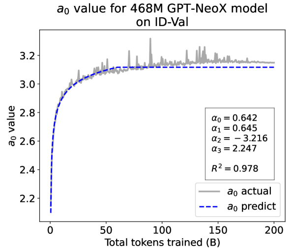
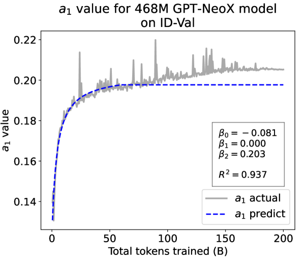
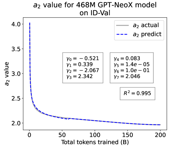
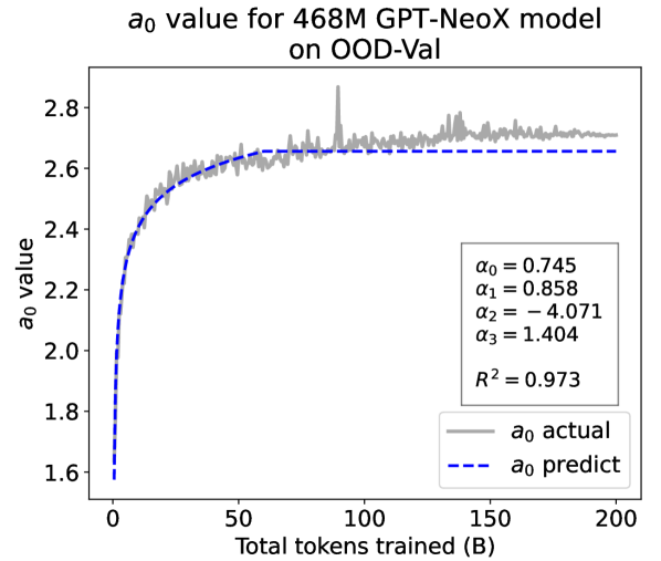
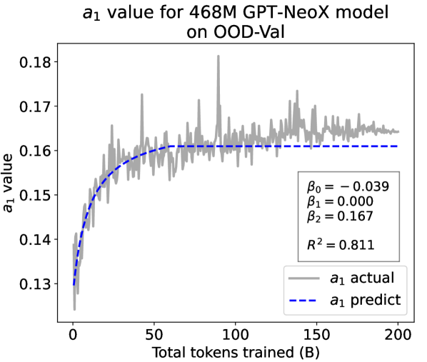
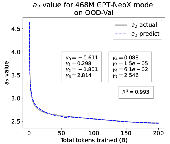
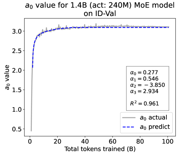
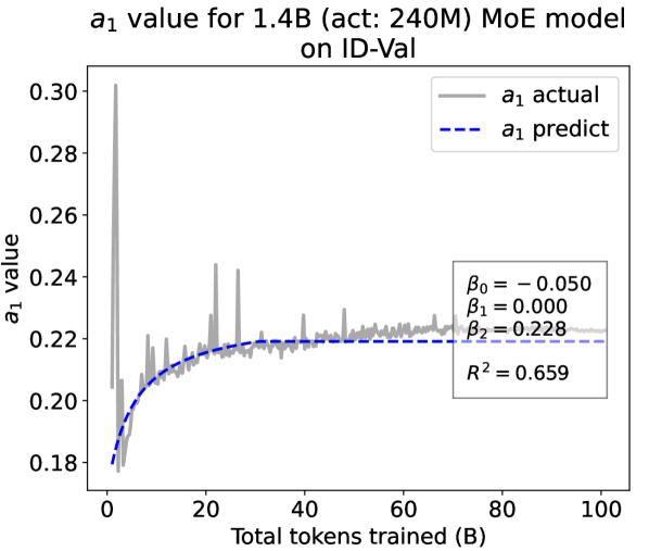
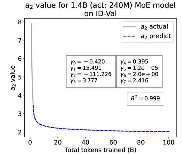
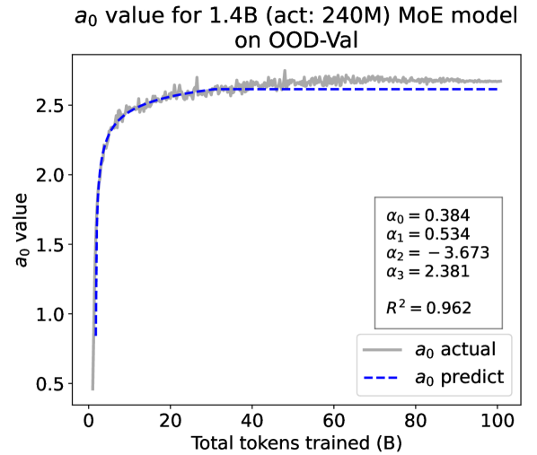
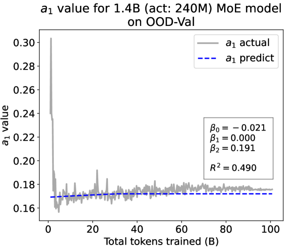
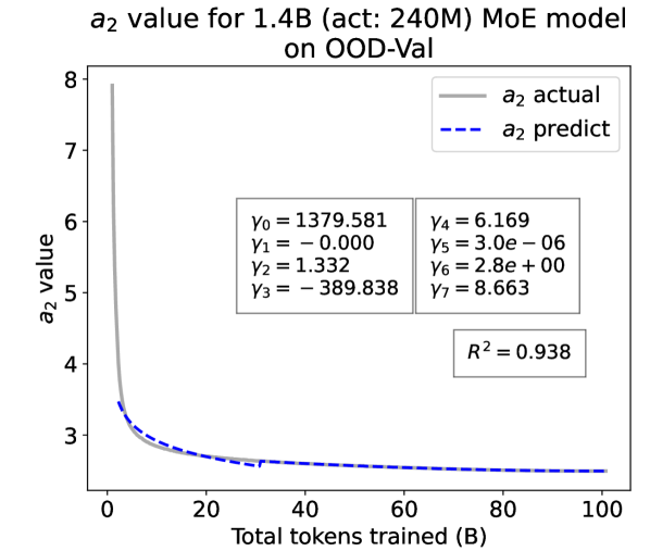
To demonstrate the generalizability of the Temporal Scaling Law to other model structures, we pre-trained a 468M model based on the GPTNeoXForCausalLM Andonian et al. (2023) architecture and a 1.4B MoE model with 240M activated parameters based on the LLaMA architecture.
Experimental Setup. The 468M GPTNeoXForCausalLM model shares the same hyperparameters with the 468M LLaMA-based model listed in Tab. 5. The 1.4B MoE model is built based on the LLaMA architecture with 16 total experts and adopts a Top-2 activation strategy, following the common setting in various MoE research Su et al. (2024a, b); Huang et al. (2024). Both models are pre-trained on the Pile dataset used in the main article. Specifically, the 468M GPTNeoXForCausalLM model is pre-trained with 200B tokens, and the 1.4B MoE model is pre-trained with 100B tokens. Detailed settings are listed in Tab. 6.
Experiment Results. We present the fitting results on both ID-Val and OOD-Val of the two pre-trained models in Fig. 4. The proposed temporal scaling law successfully genralizes to those architectures, capturing the primary patterns of parameter evolution for the GPT-NeoX and the MoE models, well demonstrating its generalizability.
Appendix G Test Loss Prediction Results on OOD-Val
In Fig. 3, we presented the test loss prediction results on the ID-Val for the scaled-up larger models. Additionally, we present the prediction results on the OOD-Val in Fig. 5. Same with results on the ID-Val, our temporal scaling law consistently generates reliable results over the comparing baselines.
Appendix H More Details for Use Case #1: Hyperparameter Selection
Due to the page limit, we omitted some details for the use case #1 in Section 4 in the article. They are thoroughly described below for reproducibility.
58M Model Architecture. The architecture of the 58M model is identical to the 70M parameter model outlined in Biderman et al. (2023). The differences between model parameters can be ascribed to different vocabulary sizes and different activation functions (i.e., SwiGLU v.s. GeLU).
Proportion Candidate Generation. In the retrieval stage, we generate a group of proportion candidates by conducting grid search on domain weights in the Pile dataset Gao et al. (2021). Specifically, we first calculate the original domain weight according to the original epoch settings noted by Gao et al. (2021) on our applied 32k tokenizer. Note that this is also the domain weight applied in Section 3.2 of the article. For the grid search, we adopt a simple but popular pipeline by selecting a domain, modifying its domain weight by a random value , and normalizing the domain weight in other domains.
Candidate Selection on the 58M Model. In the retrieval stage, we choose the Top-5 data mixture proportions on the 58M model for the rerank stage and locate the Top-1 proportion on the 58M model for final comparisons. We choose the Top-5 and Top-1 proportions by calculating the average benchmark performance of the corresponding 58M model under 0-shot, 1-shot, and 5-shot settings.
Appendix I More Details for Use Case #2: Revisit the Training Strategy
In Section 5 of the article, we have stressed that a fundamental bias in learning difficulty based on token position exists. Specifically, head tokens (with shorter context) are generally harder to predict than tail tokens (with longer context), due to the increased uncertainty caused by limited contextual information available for earlier tokens in a sequence. Surprisingly, our temporal scaling law suggests that LLMs learn equally on different token positions after an early training period (as shown by Equation 17 in the article), despite the learning difficulty bias.
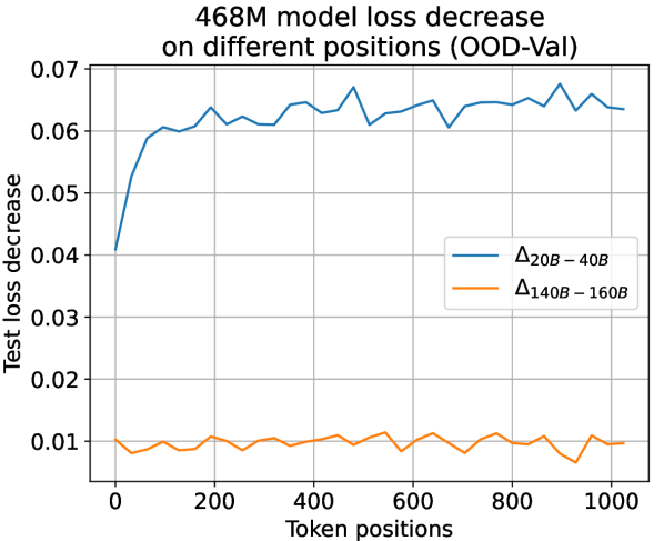
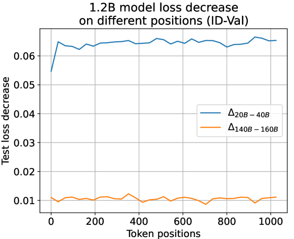
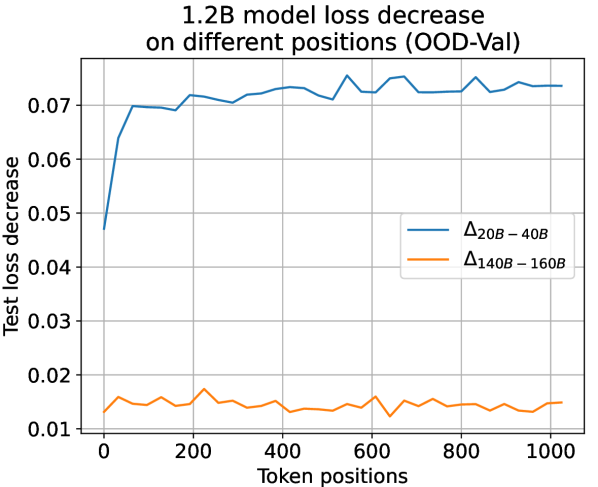
Observation for Actual Loss Decrease on Positions. We use the larger 468M and the 1.2B models to validate our suggestion. To validate this observation, we plot the actual loss decrease pattern observed during training along different token positions in Fig. 11. As shown in Fig. 11, in the early training period of “from 20B to 40B tokens”, the head tokens suffer from less loss decrease due to a higher learning difficulty. However, after the early training period, in a later period of ”from 140B to 160B tokens” that the separation point conditions in Equation 7 in the article are already fulfilled, test loss decrease among all token positions tends to be uniform across all settings. Therefore, we can infer from this observation that the learning dynamics derived from our temporal scaling law are authentically presented in LLM pre-training.
Insights for Weighting Strategies. We hypothesize that the default strategy for training generative language models, in which losses on tokens in all positions are simply averaged, is an effective solution. To validate the hypothesis, we conduct LLM pretraining on the larger 468M and the 1.2B models with three position-based weighting strategies: Head suppression, Body suppression, and Tail suppression, applied only after the point. The implementation details of these strategies are described in Tab. 9. Note that for the Suppression strategies, we normalize the weighted losses to ensure the average weight for each token position is 1.0, and thus make the corresponding average loss comparable with the default practice. We apply the pre-training settings as in Section 3.2 of the article for comparing different position-based weighting strategies. As shown in Tab. 10, despite being weighted on different token positions, weighting different tokens by position during LLM pretraining probably cannot yield better results than the default practice, though different positions possess fundamental bias in learning difficulty.
To further validate that the default practice actually trains a competitive model compared to the weighting strategies, we test the model performance on the Common Sense Reasoning benchmark described in Section 4 of the article, and report average model performance on 0-shot, 1-shot, and 5-shot settings. As shown in Tab. 11, all position-based weighting strategies acquire comparable or slightly inferior average results to the default practice, in which no weighting strategies are attached. On individual tasks, the default practice even achieves top-2 accuracies among 11 of 14 settings, surpassing all weighting variants. This indicates that weighting different tokens by position during LLM pre-training probably cannot yield better results than the default training strategy, further demonstrating that it is unnecessary to re-weight tokens by their positions during LLM pre-training.