TESS-Keck Survey V. Twin sub-Neptunes Transiting the Nearby G Star HD 63935
Abstract
We present the discovery of two nearly identically-sized sub-Neptune transiting planets orbiting HD 63935, a bright ( mag), sun-like () star at 49 pc. TESS identified the first planet, HD 63935 b (TOI-509.01), in Sectors 7 and 34. We identified the second signal (HD 63935 c) in Keck HIRES and Lick APF radial velocity data as part of our followup campaign. It was subsequently confirmed with TESS photometry in Sector 34 as TOI-509.02. Our analysis of the photometric and radial velocity data yields a robust detection of both planets with periods of and days, radii of and , and masses of and . We calculate densities for planets b and c consistent with a few percent of the planet mass in hydrogen/helium envelopes. We also describe our survey’s efforts to choose the best targets for JWST atmospheric followup. These efforts suggest that HD 63935 b will have the most clearly visible atmosphere of its class. It is the best target for transmission spectroscopy (ranked by Transmission Spectroscopy Metric, a proxy for atmospheric observability) in the so-far uncharacterized parameter space comprising sub-Neptune-sized (2.6 4 ), moderately-irradiated (100 1000 ) planets around G-stars. Planet c is also a viable target for transmission spectroscopy, and given the indistinguishable masses and radii of the two planets, the system serves as a natural laboratory for examining the processes that shape the evolution of sub-Neptune planets.
1 Introduction
Extremely rapid growth in the number of known transiting planets, thanks in large part to the Kepler and K2 missions (e.g. Batalha et al., 2013; Thompson et al., 2018; Crossfield et al., 2016; Kruse et al., 2019), has enabled population-level studies based on bulk properties like orbital period and size. One of the striking features of the population is that the mode of the radius distribution lies near 2.5– a class of planets lacking in the architecture of our own solar system. These super-earths and/or mini-neptunes bridge the size domain of terrestrials and ice giants in our solar system.
Occurrence rate distributions of these “bridge” planets exhibit additional features in the period-radius plane. For example, a feature of particular relevance to this work is the so-called “radius cliff”, a steep drop in planet occurrence between 2.5 and 4.0 R⊕ (Borucki et al., 2011; Howard et al., 2012; Fulton et al., 2017) for planets interior to 1AU. Both planets described in this paper fall in this radius regime. As well, the so-called “super-Earth” (1-1.8 R⊕) and “sub-Neptune” (1.8-4 R⊕) exoplanets are the modes of the known planet radius distribution within these bridge planets (Fulton et al., 2017), a conclusion supported by modelling (e.g. Owen & Wu, 2017). Description of the population in relation to the radius “cliff” and “valley” has become ubiquitous since their discovery.
As theoretical understandings have matured with acquisition of mass information, a variety of origins for the radius cliff have been proposed. Kite et al. (2019) propose atmospheric sequestration into magma as the cause, as larger atmospheres achieve the critical base pressure necessary to dissolve H2 from the atmosphere into the core. Work is still ongoing to understand how atmospheric observables vary across these features in order to better grasp their underlying physics. Atmospheric characterization of the planets described in this paper could help provide support for theories of the causes of the radius cliff.
Though confirmed multi-planet systems are only a subset of the full planet sample, substantial work has been done to understand the properties of such systems. Weiss et al. (2018) identify the “peas in a pod” phenomenon in the Kepler sample, which describes the fact that planets of a given size are more likely to have neighbors of a similar size than a random size. The nearly-identical planets in the HD 63935 system conform to this trend. They also identify a trend towards denser inner planets, which may be related to photoevaporation.
Mass measurements are resource intensive to obtain, in particular for the dim host stars common in the Kepler sample, but they are crucial to understanding the population in detail. Early mass measurements by Weiss & Marcy (2014) demonstrated that Kepler planets above 1.8whose stars were sufficiently bright for RV followup appear to retain substantial H/He envelopes. This is in agreement with theoretical predictions for that size regime (Lopez & Fortney, 2014). There has since been a great deal of additional work establishing relations between planetary mass and radius, though for any given planetary radius there is a wide spread in masses, implying substantial compositional diversity (e.g. Rogers, 2015; Wolfgang et al., 2016; Chen & Kipping, 2016; Zeng et al., 2019).
Efforts to understand the sub-Neptune population are being supported by the Transiting Exoplanet Survey Satellite (TESS) mission (Ricker et al., 2014). Because TESS is observing bright, nearby stars, among the planets it identifies we expect many high-quality atmospheric targets. One of the TESS Level 1 science goals is to ensure that the masses of 50 planets with radii less than 4 are measured. In doing so, we will begin to better understand the processes shaping the underlying distributions of exoplanets. The first TESS catalog paper was recently released, documenting 2241 transiting candidates from the mission (Guerrero et al., 2021). Ongoing followup work, including that undertaken by our group, the TESS -Keck Survey, continues to release well-determined masses for TESS planets.
The TESS-Keck Survey (TKS) is a consortium performing precise radial velocity followup of TESS planet candidates (Dalba et al., 2020; Weiss et al., 2021; Dai et al., 2020; Rubenzahl et al., 2021). One of our group’s primary science goals is measuring a diverse set of planet masses at high enough precision to be suitable for atmospheric characterization (Batalha et al., 2019), in particular with JWST , which is what led us to observe HD 63935. One relevant axis of diversity is in host star spectral type. So far, only one sub-Neptune sized planet around a G star has been the subject of an atmospheric characterization study (HD 3167 c - Mikal-Evans et al. (2020)). Because of their relatively small transit signals, such planets represent more challenging targets than similar-sized targets around M or K dwarfs. However, the brightness of the host stars can compensate for this, and a number of compelling targets for atmospheric characterization with JWST around G star hosts have already emerged from TESS (e.g. Gandolfi et al., 2018; Mann et al., 2020; Weiss et al., 2020, Lubin et. al.; in prep, Turtelboom et. al., in prep).
HD 63935 b, the subject of this paper, is one of the planets we identified as a compelling atmospheric target around a G-type host star. HD 63935 is a bright (V) G5 star at a distance of 49 pc. Study of planets around this class of star is valuable to help understand how differences in host star characteristics shape planet formation. With atmospheric data, we will be able to test theoretical predictions like those of Lopez & Fortney (2014), that H/He mass fraction is primarily a function of radius. Characterizing these planets will also be valuable for comparative studies with our own solar system. Although we have not discovered any planetary systems that closely resemble our own, the reasons for this are likely observational (Martin & Livio, 2015). A better understanding of what makes our solar system unique (or not) is important to the search for life.
In this paper, we present the confirmation of the sub-Neptune planets HD 63935 b and c. Planet b is uniquely well-suited to atmospheric characterization, being the second-best target on the radius cliff and the best in its niche of sub-Neptune-sized (2.6 4 ), moderately-irradiated (100 1000 ) planets around G-stars. Planet c is also amenable to atmospheric characterization. We also discuss evidence for a longer-period planetary mass companion to the two confirmed planets, though we ultimately adopt a two-planet model. In Section 2, we describe the selection algorithm that our consortium’s atmospheres working group uses to select high-quality targets. In Section 3 we provide a description of our efforts to characterize the planets’ host star. In Section 4, we will describe the observations we undertook to confirm this planetary system. In Section 5, we will provide details of our analysis and results, and in Section 6 discuss their implications.
2 The TESS-Keck Survey: Atmospheric Target Selection
This work is based on data obtained as part of the TESS-Keck Survey (TKS), which performs precise radial velocity (PRV) follow-up of TESS planet candidates using the Keck telescope on Mauna Kea and the APF telescope at Lick Observatory. As part of TKS, we are interested in selecting the TESS planet candidates that would represent the best prospects for atmospheric characterization. TESS has produced (and continues to produce) far too many promising atmospheric targets for one consortium to follow up. Consequently, we attempted to develop an algorithm to prioritize targets to add to our PRV prioritized observing list; see Chontos et. al. (in prep.) for more details about the general selection of TKS targets.
Our algorithm aims to find high quality atmospheric targets in regions of parameter space mostly bereft of them. We select mostly planets in the sub-Neptune regime, as many highly-observable giant planets are already known and terrestrial planets are, with a few exceptions, not accessible with JWST. As a quantification of “under-populated parameter space,” our selection algorithm bins planets in stellar effective temperature, planet radius, and insolation flux. We then select targets that stand out in bins without any characterized planets. A detailed explanation of the algorithm follows.
The inputs to our algorithm are the star and planet properties from NASA Exoplanet Archive111https://exoplanetarchive.ipac.caltech.edu/ and the TESS TOI list222https://tev.mit.edu/data/collection/193. We subject these lists to certain cuts as well as manual inspections of the data validation reports (Twicken et al., 2018). We exclude TOIs with declination or V for visibility at our facilities and to ensure acceptable SNR, respectively. We also cut planets with R R⊕, as the Jovian population is already reasonably well-sampled (for the atmospheres science case only - TKS as a whole does follow up some large planet candidates). We also exclude stars with T 6500 K.
After our initial culling of the sample, we calculate an estimated mass for each TESS planet candidate based on the fitting formulae of Chen & Kipping (2016) and Weiss & Marcy (2014). With that, we calculate a Transmission Spectroscopy Metric (TSM) value (Kempton et al., 2018). This value is an estimate for the Signal-to-Noise Ratio (SNR) of a planet candidate’s atmosphere as observed with the NIRISS instrument on the James Webb Space Telescope. For our purposes, it serves as a proxy for relative observability.
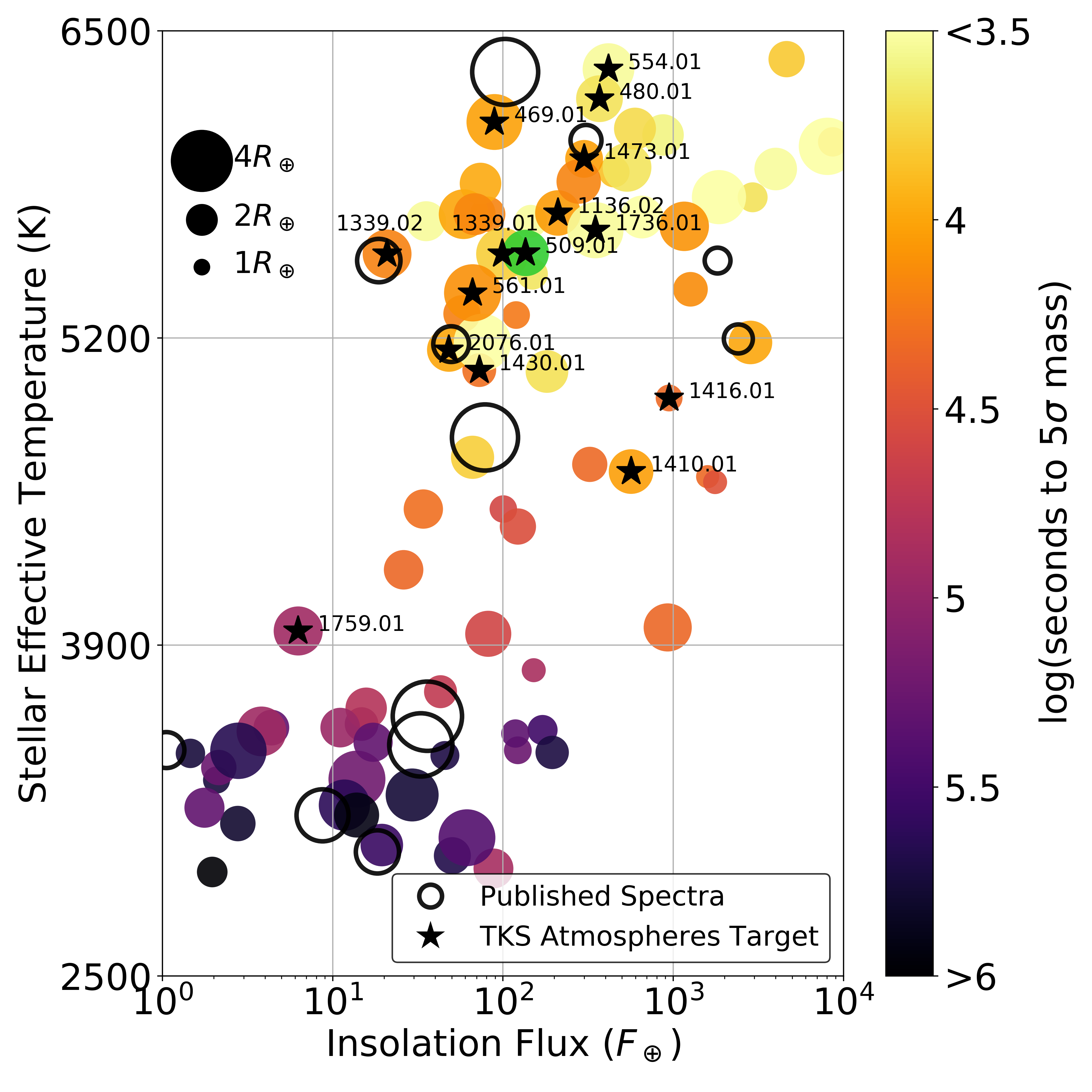
Our selection algorithm then computes a final parameter, which is equal to the TSM value normalized by the expected exposure time on HIRES that would be required to obtain a mass precision better than 20%, estimated based on Plavchan et al. (2015). This metric was chosen as our ranking parameter in order to select a reasonably large sample of planets. Ranking by TSM alone results in HIRES time spent on M stars, which is sub-optimal for a visual light spectrograph. Cool stars are better suited to characterization by instruments at other facilities like MAROON-X (Seifahrt et al., 2018) or CARMENES (Quirrenbach & Consortium, 2020), which have more sensitivity in the red. See fig. 1, which plots the most promising atmospheric targets from TESS with their estimated time to measure the mass with a precision of 20%, for a visual representation of this.
With all relevant metrics calculated, our algorithm divides planets into bins along three axes in parameter space: planet radius, stellar effective temperature, and insolation flux. We use five log-uniform radius bins (which conveniently includes edges at 1.7 R⊕, approximately the location of the radius gap, and 4 R⊕, dividing the sub- and super-Neptune populations), five log-uniform insolation flux bins, and three stellar effective temperature bins, resulting in 75 bins total, some of which were unpopulated. TOIs that had higher X metric values than other TOIs and known planets in their bin were prioritized for our PRV observing list. There were enough planet candidates meeting this criteria that we could not observe them all, and as a result we focused on those with the highest X metrics. Our algorithm permitted the removal of candidates deemed observationally unsuitable, e.g. by spectral signatures suggestive of an eclipsing binary, or by substantial stellar activity making continued observations infeasible. This selection process is what led us to observe HD 63935, the subject of this paper, which remains the highest-ranked target in its bin by X metric.
3 Host Star Characterization
We obtained high resolution spectra of HD 63935 (HIP 38374, TIC 453211454; other aliases in Table 1). We used SpecMatch-Syn (Petigura et al., 2017) to obtain stellar effective temperature, , and metallicity. We then used these values, combined with luminosity and parallax from Gaia (Prusti et al., 2016; Collaboration et al., 2020), as priors to obtain the stellar mass, radius, and age using isoclassify (Huber et al., 2017; Berger et al., 2020) (Table 3). isoclassify functions by using the input parameters stated above to fit the star to a curve of constant age (isochrone) in the relevant parameter space, allowing the calculation of a radius, mass, and age value. We add a 4% and 5% systematic uncertainty to the stellar radius and mass values, respectively, to account for isochrone grid uncertainty, following Tayar et al. (2020). Note that our derived age does not account for these uncertainties. The values we obtain for mass and radius are consistent with those provided by SpecMatch Synth, those derived by the Gaia mission (Collaboration et al., 2020), and those from our spectral energy distribution fitting. The star is slightly smaller than the Sun (R∗=0.959R⊙, M∗=0.933R⊙), and its isoclassify-derived age suggests that the system is older as well, at Gyr. This is consistent with our nominally low value of km s-1 and low activity indicator R’HK = -5.06, suggestive of an old, relatively inactive star. The two sectors of TESS photometry do not provide enough information to obtain a reliable rotation period estimate, though we discuss other methods for obtaining this value in Section 3.2.
| Aliases | |
|---|---|
| HIP ID | 38374 |
| TIC ID | 453211454 |
| Tycho ID | 783-536-1 |
| Gaia EDR3 ID | 3145754895088191744 |
| Gaia 6D Solution | |
| Right Ascension | 07:51:42.04 |
| Declination | +09:23:11.40 |
| Parallax | 20.470 0.019 mas |
| RA Proper Motion | -78.696 0.022 mas yr-1 |
| Dec Proper Motion | -188.512 0.013 mas yr-1 |
| Radial Velocity | -20.34 0.19 km s-1 |
3.1 Spectral Energy Distribution and Activity
As an independent determination of the stellar parameters, we also performed an analysis of the broadband spectral energy distribution (SED) of the star together with the Gaia EDR3 parallaxes, in order to determine an empirical measurement of the stellar radius, following the procedures described in Stassun & Torres (2016); Stassun et al. (2017, 2018). We obtained the magnitudes from Tycho-2, the Strömgren magnitudes from Paunzen (2015), the magnitudes from 2MASS, the W1–W4 magnitudes from WISE, the magnitudes from Gaia, and the FUV and NUV magnitudes from GALEX. Together, the available photometry spans the full stellar SED over the wavelength range 0.15–22 m (see Figure 2).
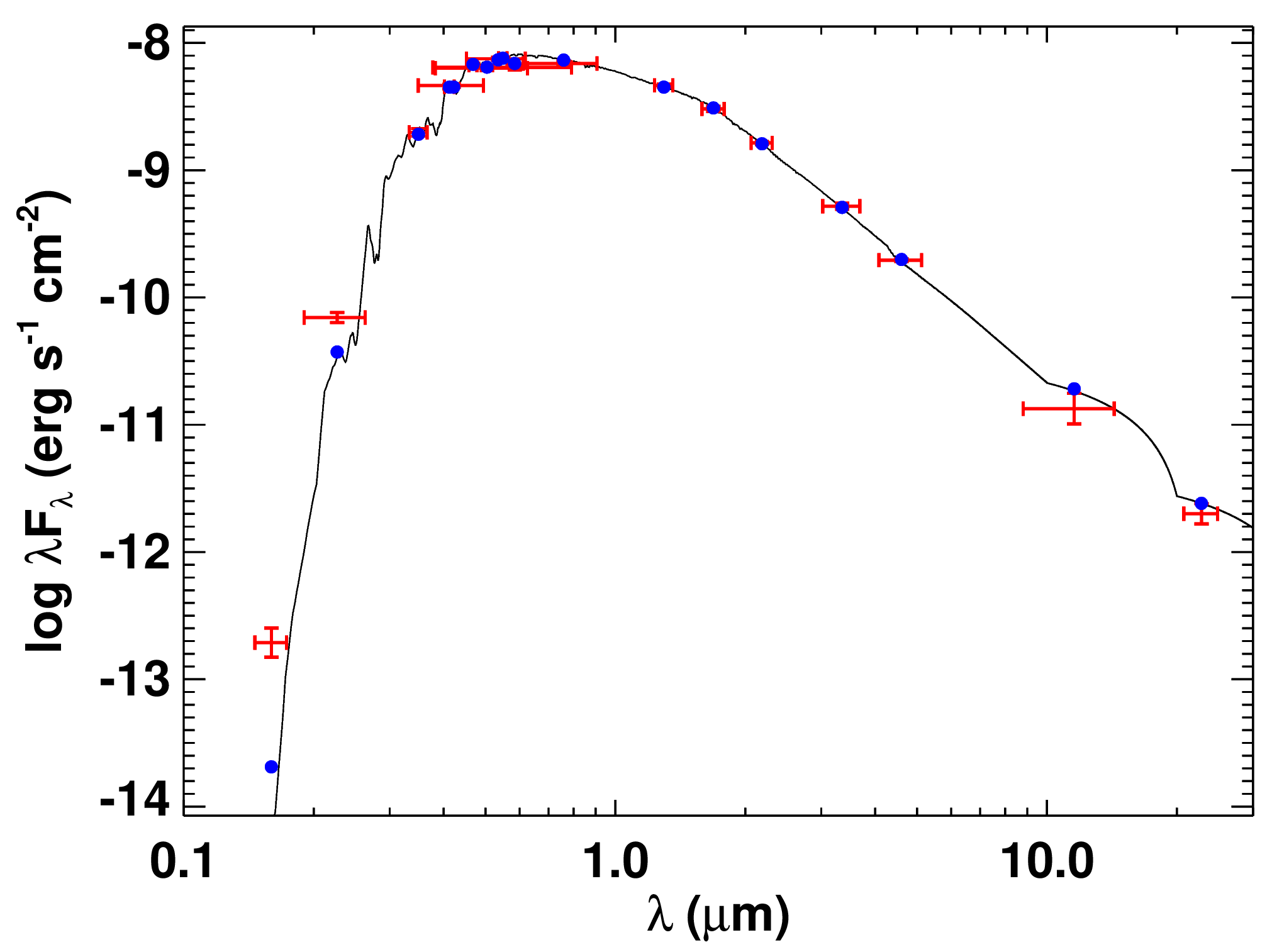
We performed a fit using Kurucz stellar atmosphere models, with the effective temperature (), metallicity ([Fe/H]), and surface gravity () adopted from the spectroscopic analysis. The only additional free parameter is the extinction (), which we restricted to the maximum line-of-sight value from the dust maps of Schlegel et al. (1998). The resulting fit is very good (Figure 2) with a reduced of 1.1 and best-fit . Integrating the (unreddened) model SED gives the bolometric flux at Earth, erg s-1 cm-23. Taking the and together with the Gaia EDR3 parallax, gives the stellar radius, . In addition, we can use the together with the spectroscopic to obtain an empirical mass estimate of , which is consistent with that obtained via empirical relations of Torres et al. (2010), . These parameters are also consistent with those we derive from isoclassify. Finally, the and together yield a mean stellar density of g cm-3.
3.2 Predicted Rotation Period from Gyrochronology
Before photometry confirmed the existence of HD 63935 c as a transiting planet, we were interested in obtaining the stellar rotation period in order to rule that out as the source of the radial velocity signal at 21 days. Although the TESS Sector 34 photometry has since confirmed that candidate, we include the following gyrochronology analysis in the text as it provides novel information about the host star. We used Markov Chain Monte Carlo (MCMC) within kiauhoku (Claytor et al., 2020) to obtain a posterior probability distribution of stellar parameters for HD 63935. For input we used Gaussian priors based on the spectroscopic effective temperature and metallicity, as well as the isoclassify-derived age. Assuming a gyrochronological model, we were then able to predict the rotation period. We performed MCMC using two different braking laws on the same grid of stellar models: one (“fastlaunch”) uses the magnetic braking law presented by van Saders & Pinsonneault (2013), while the other (“rocrit”) uses the stalled braking law of van Saders et al. (2016). With the fastlaunch model, we predicted days, while we predicted days using the rocrit model. Both of these are consistent with a star somewhat older than the sun, as implied by our measured R’HK value and derived via isoclassify, as well as our non-detection of a rotation period in the TESS data.
4 Observations
4.1 TESS Photometry
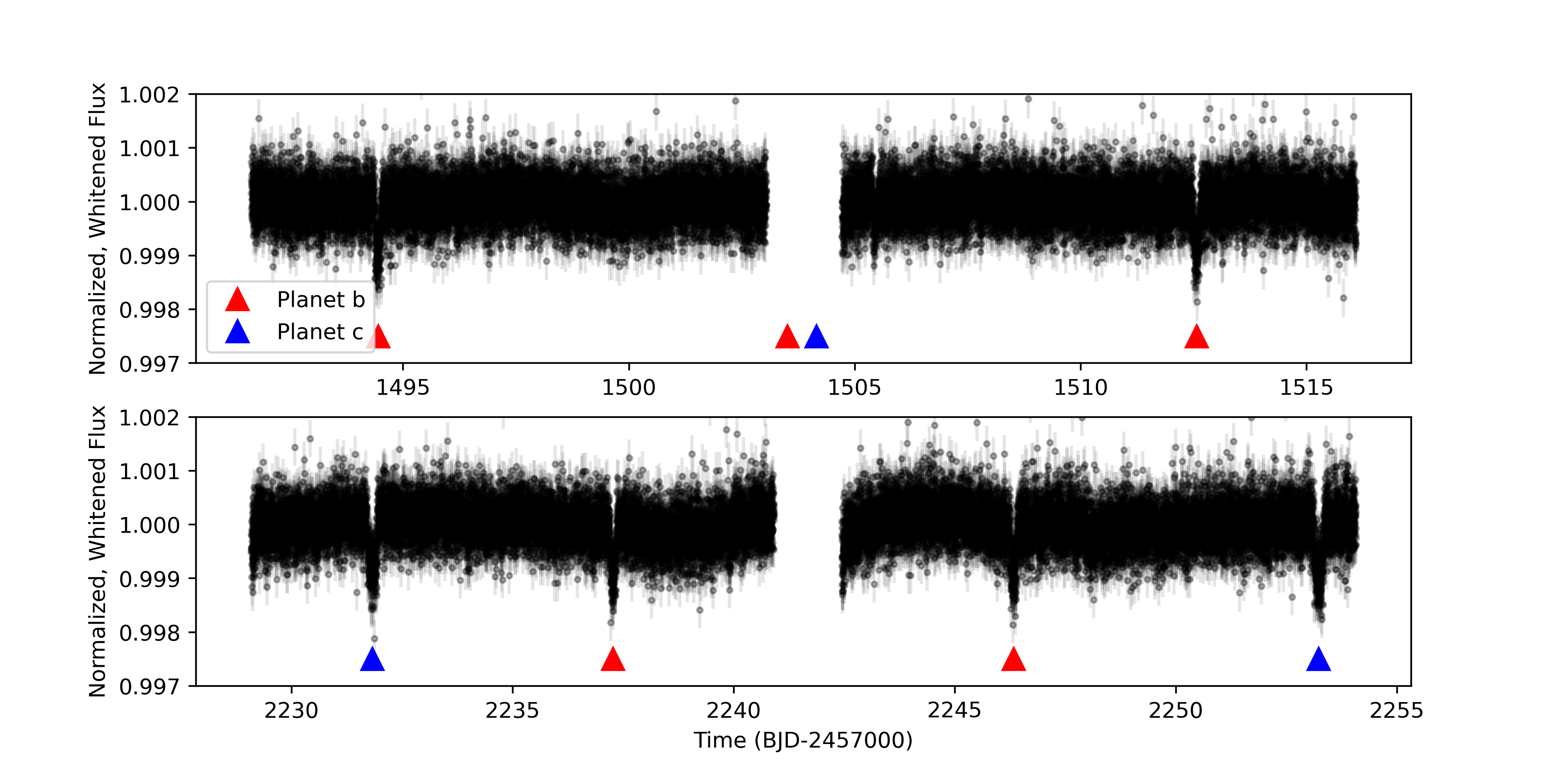
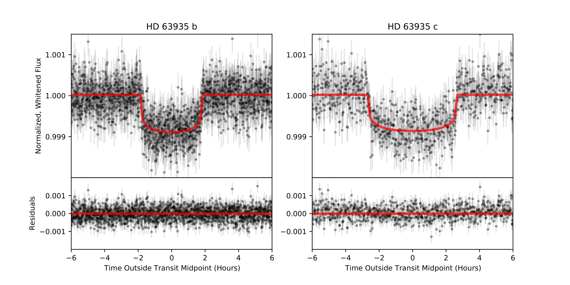
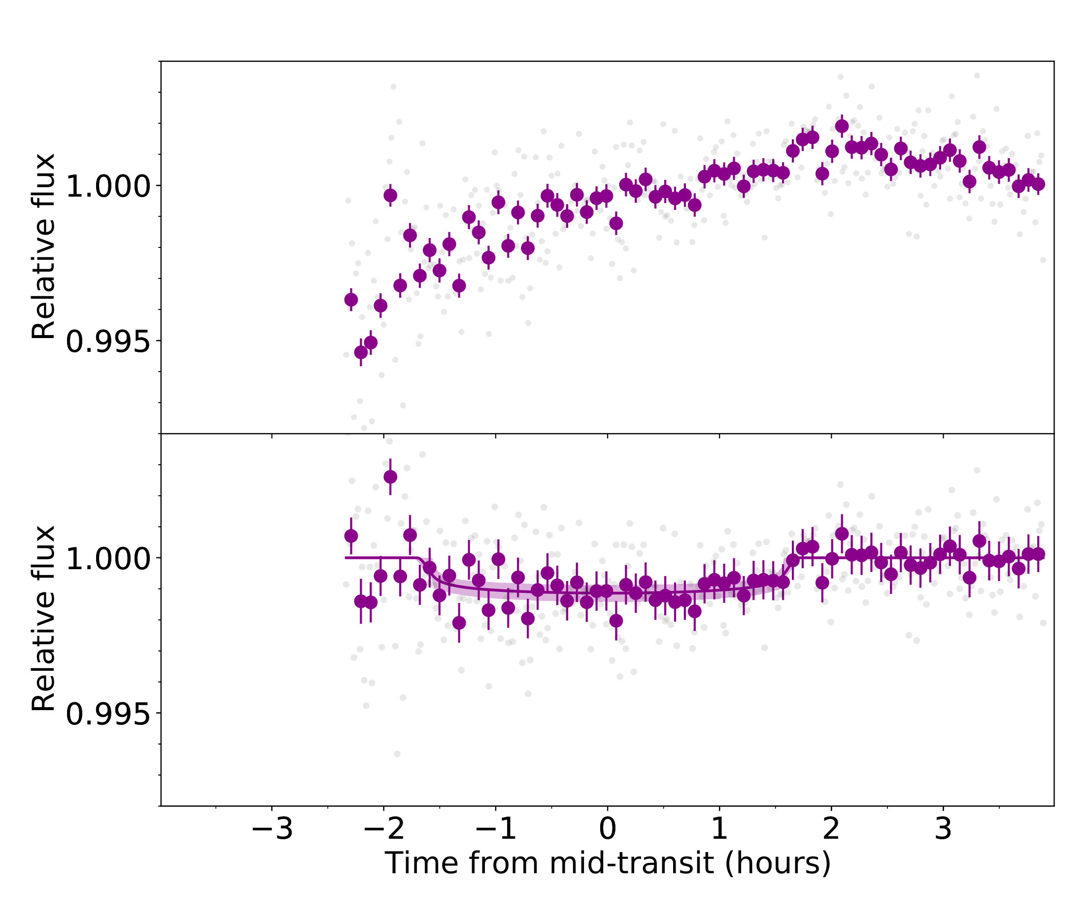
HD 63935 (TIC 453211454, TOI 509) was observed by the TESS mission in sector 7 between UT 2019 January 7 and 2019 February 2, and sector 34 between UT 2021 January 13 and 2021 February 9. The star was imaged by CCD 4 of Camera 1. The data consist of 33208 data points with integration times of two minutes each. The Science Processing Operations Center (Jenkins et al., 2016) processed the data, generated light curves using Simple Aperture Photometry (SAP Twicken et al., 2010; Morris et al., 2020), and removed known instrumental systematics using the Presearch Data Conditioning (PDCSAP) algorithm (Smith et al., 2012; Stumpe et al., 2012, 2014). The Sector 7 data contained two transits of planet b, and the Sector 34 data contained two additional transits of planet b and two transits of planet c. The transit of planet c that occurred during Sector 7 happened during a gap in the TESS lightcurve (see Section 5.1. For the analysis described here, we downloaded the PDCSAP flux data from the publicly-accessible Mikulski Archive for Space Telescopes (MAST)333https://archive.stsci.edu/tess/. The full light curve is plotted in Figure 3 and the phase-folded transits in Figure 4.
4.2 AO Imaging
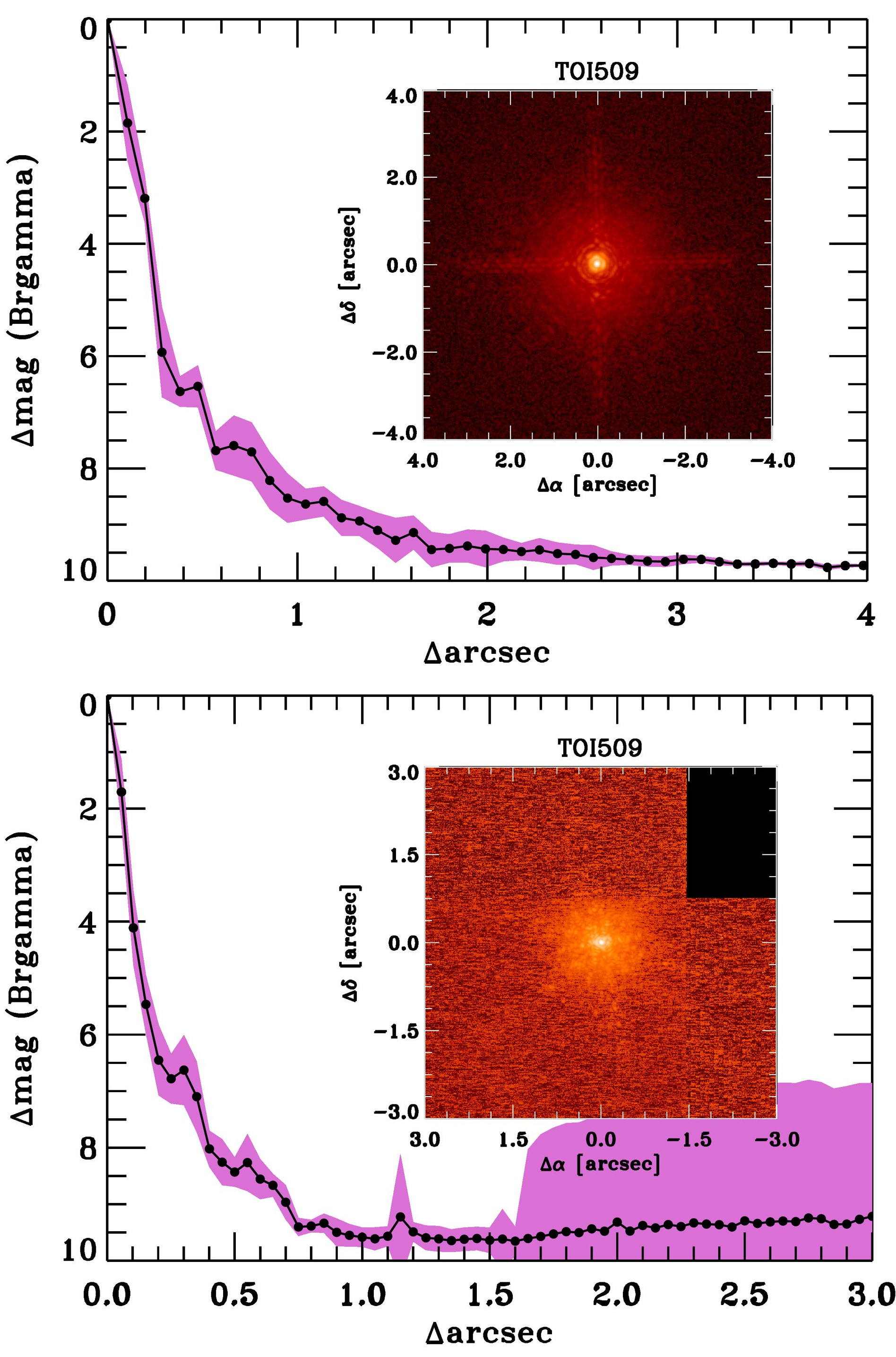
As part of our standard process for validating transiting exoplanets to assess the the possible contamination of bound or unbound companions on the derived planetary radii (Ciardi et al., 2015), we observed TOI-509 with high-resolution near-infrared adaptive optics (AO) imaging at Palomar and Keck Observatories.
The Palomar Observatory observations were made with the PHARO instrument (Hayward et al., 2001) behind the natural guide star AO system P3K (Dekany et al., 2013) on 2019 Apr 18 UT in a standard 5-point quincunx dither pattern with steps of 5″ in the narrow-band filter m). Each dither position was observed three times, offset in position from each other by 0.5″ for a total of 15 frames; with an integration time of 1.4 seconds per frame, the total on-source time was 21 seconds on target. PHARO has a pixel scale of per pixel for a total field of view of . These observations were taken at an airmass of 1.1858.
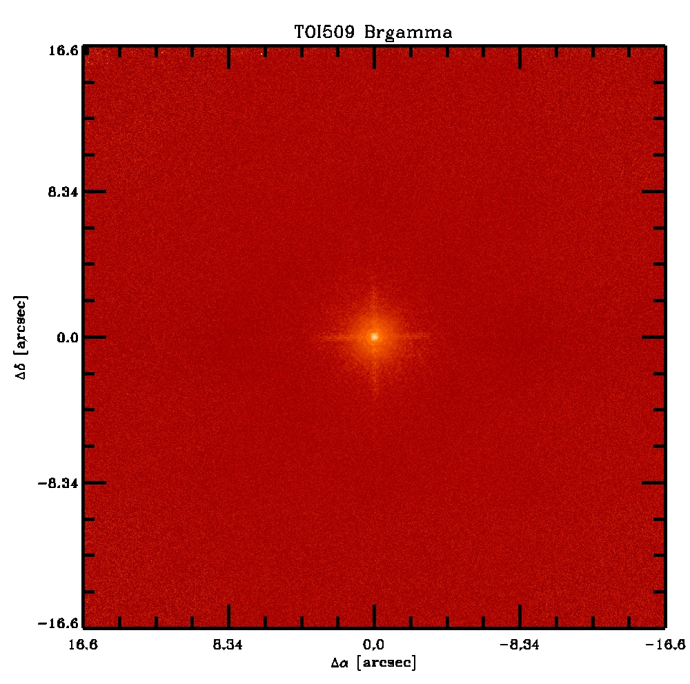
The Keck Observatory observations were made with the NIRC2 instrument on Keck-II behind the natural guide star AO system (Wizinowich et al., 2000) on 2019-Mar-25 UT in the standard 3-point dither pattern that is used with NIRC2 to avoid the left lower quadrant of the detector which is typically noisier than the other three quadrants. The dither pattern step size was and was repeated twice, with each dither offset from the previous dither by . NIRC2 was used in the narrow-angle mode with a full field of view of and a pixel scale of approximately per pixel. The Keck observations were made in the narrow-band filter m) with an integration time of 0.5 second for a total of 4.5 seconds on target. Observations were taken in narrow camera mode with a 1024” x 1024” FOV and at an airmass of 1.43.
The AO data were processed and analyzed with a custom set of IDL tools. The science frames were flat-fielded and sky-subtracted. The flat fields were generated from a median average of dark subtracted flats taken on-sky. The flats were normalized such that the median value of the flats is unity. The sky frames were generated from the median average of the 15 dithered science frames; each science image was then sky-subtracted and flat-fielded. The reduced science frames were combined into a single combined image using a intra-pixel interpolation that conserves flux, shifts the individual dithered frames by the appropriate fractional pixels, and median-coadds the frames (Figure 6). The final resolution of the combined dithers was determined from the full-width half-maximum of the point spread function; 0.094″ and 0.050″ for the Palomar and Keck observations respectively.
4.3 Ground-Based Photometry
The TESS pixel scale is pixel-1, and photometric apertures typically extend out to roughly 1 arcminute, which generally results in multiple stars blending in the TESS aperture. An eclipsing binary in one of the nearby blended stars could mimic a transit-like event in the large TESS aperture. We conducted ground-based photometric follow-up observations as part of the TESS Follow-up Observing Program (TFOP)444https://tess.mit.edu/followup with much higher spatial resolution to confirm that the transit signal of HD 63935 b is occurring on-target, or in a star so close to HD 63935 that it was not detected by Gaia DR2.
4.3.1 MuSCAT
We observed one partial transit of HD 63935 b on 2019 March 24 from 10:29 to 15:09 in UTC covering the expected egress, with the multi-color simultaneous camera MuSCAT (Narita et al., 2015), which is mounted on the 1.88 m telescope of the Okayama Astronomical Observatory in Okayama, Japan. MuSCAT has three optical channels each equipped with a 1024x1024 pixels CCD camera, enabling g-, r-, and zs-band simultaneous imaging. Each camera has a pixel scale of per pixel, providing a field of view (FOV) of 6.1×6.1″. The exposure times were (10, 3, 3) sec for g, r, zs-bands, respectively.
We performed standard aperture photometry using the custom photometry pipeline described in detail in Fukui et al. (2011). The adopted aperture was 20 pixels or 7″which excludes any nearby stars as the source of the signal of HD 63935 b. Our precision was not enough to detect the expected 0.09% transit signal on target in each band, but the data ruled out deep eclipses in all nearby stars within the field of view that are consistent with the transit depth from TESS.
4.3.2 LCOGT
We observed a full transit of HD 63935 b in the Pan-STARRS filter (central wavelength 1004 nm) on UTC 2020-11-20 from the Las Cumbres Observatory Global Telescope (LCOGT) (Brown et al., 2013) 1.0 m network node at McDonald Observatory. We used the TESS Transit Finder, which is a customized version of the Tapir software package (Jensen, 2013), to schedule our transit observations. The LCOGT SINISTRO cameras have an image scale of per pixel, resulting in a field of view. The images were calibrated by the standard LCOGT BANZAI pipeline (McCully et al., 2018), and photometric data were extracted with AstroImageJ (Collins et al., 2017). The images were focused and have typical stellar point-spread-functions with a full-width-half-maximum (FWHM) of , and circular apertures with radius were used to extract the differential photometry. The light curve is presented in Figure 5.
4.4 Ground-Based Spectroscopy
4.4.1 LCO NRES
We obtained a spectrum of the target with the automated LCOGT 1m/NRES optical (380-860) spectrograph (Brown et al., 2013; Siverd et al., 2018), in order to characterize the star and look for signs of a stellar binary system. The observation was done on UT 2019 March 22, at the McDonald Observatory node of the LCOGT network. We observed the target with two consecutive 20 minute exposures that were processed by the LCO Banzai reduction pipeline (McCully et al., 2018) and then stacked together for a spectrum with an effective 40 minutes exposure time and a SNR of 73. The reduced spectrum was processed by the SpecMatch-Syn pipeline (Petigura et al., 2017) where spectral and stellar parameters were derived while accounting for the target’s distance derived from the Gaia DR2 parallax (Gaia Collaboration et al., 2018). The spectrum did not show evidence for a second set of lines, and the SpecMatch-Syn analysis showed the target is a slowly rotating ( km s-1) Sun-like star with an absolute RV ( km s-1) consistent with the Gaia DR2 RV ( km s-1).
4.4.2 TRES
We obtained two spectra, on UT 2019 March 28 and 2019 April 04, using the Tillinghast Reflector Echelle Spectrograph (TRES) on the 1.5m telescope at the Whipple Observatory on Mt. Hopkins in Arizona. TRES is an optical echelle spectrograph with a wavelength range of nm and has a resolution of (Fűrész, 2008; Mink, 2011). The two TRES observations were well-separated in orbital phase (4.21 and 4.59) of the photometric ephemeris and were used to derive relative radial velocities. Using the strongest observed spectrum as a template, the second spectrum was cross-correlated order-by-order in the wavelength range nm. The observed template spectrum was assigned a velocity of zero and the small velocity difference between the two spectra was 13 m/s, which ruled out a stellar or brown-dwarf companion as the source of the transit-like events. The TRES observations also revealed a spectrum very similar to that of the Sun, with line broadening due to rotation of less than 4 km/s and no indication of surface activity, such as emission at Ca II HK, thus confirming that this target was well suited for PRV work.
The stellar effective temperature (), metallicity ([Fe/H]), surface gravity (), and rotation () were also determined using the Stellar Parameter Classification tool (SPC) on the TRES spectra (Buchhave et al., 2012). SPC cross-correlates the observed spectra against a library of synthetic spectra calculated using Kurucz model atmospheres (Kurucz, 1993) and does a multi-dimensional fit for the stellar parameters that give the highest peak correlation value. These stellar parameter estimates are within 1 agreement with the results from the SpecMatch-Syn analysis of the PRV observations.
4.4.3 TNG/HARPS-N
Between UT 2019 April 2 and 2019 April 29 we collected 11 spectra of TOI-509 with the HARPS-N spectrograph (Cosentino et al., 2012, (383-693 nm, R115 000) mounted at the 3.58-m Telescopio Nazionale Galileo (TNG) of Roque de los Muchachos Observatory in La Palma, Spain, under the observing programmes CAT19A_162 (PI: Nowak) and CAT19A_96 (PI: Pallé). The exposure time was set to 600–900 seconds, based on weather conditions and scheduling constraints, leading to a SNR per pixel of 59–119 at 5500 Å. The spectra were extracted using the off-line version of the HARPS-N DRS pipeline (Cosentino et al., 2014), version 3.7.
Doppler measurements and spectral activity indicators (Bisector Inverse Slope (BIS), full-width at half maximum (CCF_FWHM) contrast (CCF_CTR) of the cross-correlation function (CCF), Mount-Wilson S-index and index) were measured using an on-line version of the DRS, the YABI tool555Available at http://ia2-harps.oats.inaf.it:8000., by cross-correlating the extracted spectra with a G2 mask (Baranne et al., 1996). We measure a value of -4.94. We also used serval666https://github.com/mzechmeister/serval (Zechmeister et al., 2018) to measure relative RVs, chromatic index (CRX), differential line width (dLW), and H index. The uncertainties of the relative RVs measured with serval are in the range 0.5–1.4, with a mean value of 0.83.
4.4.4 Keck HIRES
Between 2019 August and 2021 March, we obtained 51 high-resolution spectra of HD 63935 with the HIRES instrument (Vogt et al., 1994) on the 10m Keck 1 telescope at the W.M. Keck Observatory on Maunakea, Hawai’i. We obtained spectra with the C2 decker, which has dimensions of 14” x 0.86” and spectral resolution R60000 at 500 nm. The chosen exposure meter setting regulates S/N at 200 photons per pixel and the resulting median exposure time is 185 s. We obtained radial velocity measurements from the spectra using the method described in Howard et al. (2010). The RMS value of our radial velocities before fitting for any planets was 4.22 ms-1, and the median internal uncertainty was 1.1 ms-1. Our measured value is -5.04, indicating a relatively low-activity star and consistent with the value measured by HARPS-N.
4.4.5 APF-Levy
Between 2019 August and 2021 February, we obtained 100 spectra of HD 63935 with the Levy Spectrograph, a high resolution slit-fed optical (500-620nm) echelle spectrograph (Radovan et al., 2010) on the Automated Planet Finder Telescope (APF) at Lick observatory(Vogt et al., 2014). We observed the star using the W decker, which has dimensions of 3” x 1” and R114000 between 374 and 970 nm. Our median exposure time with APF was 1200 seconds. We acquired one or two observations per night. Nightly observations are binned to improve the RV precision. The RMS values of our radial velocities before fitting for any planets was 8.27 ms-1, and the median uncertainty was 1.8 ms-1. We excluded data points with RV uncertainties 5 ms-1, which resulted in the removal of five points. All such points were clear outliers and had 800 counts on the detector, indicating low data quality.
| Time (BJD) | RV (m s-1) | RV Unc. (m s-1) | Inst. |
|---|---|---|---|
| 2458733.13862 | -6.81 | 1.29 | HIRES |
| 2458744.13959 | -8.04 | 1.11 | HIRES |
| 2458777.06304 | 0.28 | 1.16 | HIRES |
| 2458788.11234 | -11.38 | 1.06 | HIRES |
| 2458795.00493 | -5.68 | 1.00 | HIRES |
A sample of the radial velocities, uncertainties, and instruments for our data on HD 63935. The full table of radial velocity data is available online, which includes the Mt. Wilson S-value activity indicators.
5 Analysis and Results
5.1 TESS Photometry Analysis
We used juliet (Espinoza et al., 2019) to model the light curve data available for HD 63935. juliet serves as a wrapper for a variety of existing publicly-available tools. Our transit modelling used the functions based on batman (Kreidberg, 2015) for transit fitting and PyMultiNest (Buchner et al., 2014) for the sampling of parameter space. We fit for both planets’ periods, crossing times, transit depths, and impact parameters, as well as two quadratic limb darkening parameters (following Kipping (2013), the out-of-transit flux, and a jitter term from TESS. We keep all other parameters fixed, including the mean stellar density, for which we fix the value to that derived in Section 3. We impose normal priors centered on the SPOC values for period and crossing time (Jenkins, 2002; Jenkins et al., 2010; Li et al., 2019), all with widths of 0.1 days, and constrain the occultation fraction and impact parameter to a uniform range between 0 and 1.
When we began to study this system, the gap in the TESS Sector 7 photometry (Sector 34 data had not been obtained yet) combined with only two transits meant that two periods ( days, the one initially reported by SPOC, and 9 days, which we ultimately selected based on RV measurements and was later confirmed by TESS S34) were possible for planet b. The Sector 7 light curve also provided no indication of the existence of planet c, as its transit fell in the data gap as well. We selected the correct period (9 days) and identified planet c as a candidate based on our radial velocity observations (see Section 5.3). Both of our predictions were validated by the Sector 34 light curve, which confirmed the 9 day period as the correct one for planet b and provided 2 transits of planet c at almost exactly the period predicted by our radial velocity data (21.40 days compared to our predicted value of 21.35 days). Both planets have high SNR transits (18.6 and 23.0 for planets b and c, respectively). The results are of these fits are reported in Table 3.
5.1.1 LCO Photometry Analysis
As a check on the orbital solution for planet b (in particular the orbit period), we performed an independent fit of the LCO lightcurve (Fig. 5, Sec. 4.3.2) using exoplanet (Foreman-Mackey et al., 2021). We fixed at the value found from the TESS lightcurve fit. The fit to the LCO lightcurve gives 68% credible intervals on the posterior values found for , , hr, and . These are consistent with the values from the TESS fit (Table 3), though the period values are consistent only within the 2- errors, and not within the 1- errors.
5.2 High Resolution Imaging
To within the limits of the AO observations, no stellar companions were detected. The sensitivities of the final combined AO image were determined by injecting simulated sources azimuthally around the primary target every at separations of integer multiples of the central source’s FWHM (Furlan et al., 2017; Lund, Submitted). The brightness of each injected source was scaled until standard aperture photometry detected it with significance. The resulting brightness of the injected sources relative to TOI 509 set the contrast limits at that injection location. The final limit at each separation was determined from the average of all of the determined limits at that separation and the uncertainty on the limit was set by the rms dispersion of the azimuthal slices at a given radial distance (Figure 7).
5.3 Radial Velocity Analysis
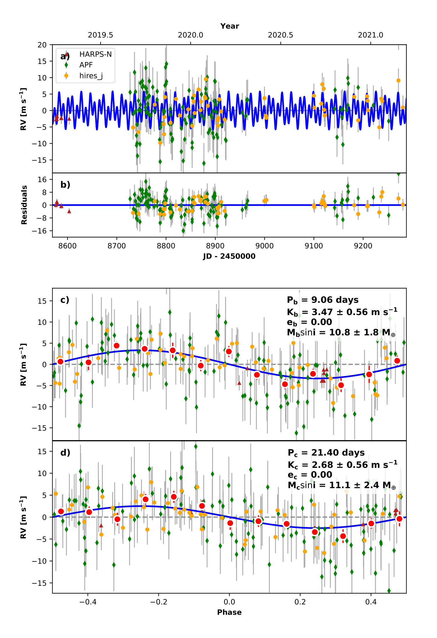
We used the RadVel777https://radvel.readthedocs.io/en/latest/ package (Fulton et al., 2018) to model the radial velocity measurements of HD 63935. RadVel uses the Markov chain Monte Carlo (MCMC) sampler emcee (Foreman-Mackey et al., 2013a) to sample the posterior space of the model’s parameters. In these fits, we fix the period and time of inferior conjunction to the values derived from photometry (previous section). We enforce circular orbits in our fits. Allowing eccentricity to vary produced a fit which was not preferred by the information criterion analysis. Varying or only were “somewhat disfavored” with AICc and AICc, respectively, while varying both eccentricities was “strongly disfavored” with AICc). If the eccentricities are allowed to vary, we find 1 upper limits of 0.16 and 0.29 for planets b and c, respectively.
Our preliminary single planet fits of this system were dominated by a signal at 21 days; we identified this signal as corresponding to an additional planet candidate, HD 63935 c, which was confirmed by two transits in TESS Sector 34. The final results of our radial velocity fits are displayed in Figure 8.
| Parameter | Symbol | Value | Units | |
|---|---|---|---|---|
| Stellar Parameters | ||||
| Mass1 | 0.933 | M⊙ | ||
| Radius1 | 0.959 | R⊙ | ||
| Age1 | 6.8 | Gyr | ||
| Stellar Effective Temperature2 | 5534100 | K | ||
| Surface Gravity2 | 0.1 | cm s-1 | ||
| Metallicity1 | [Fe/H] | dex | ||
| Activity Index2 | R’HK | -5.06 | ||
| V-band Magnitude3 | 8.58 | |||
| J-band Magnitude3 | 7.30 | |||
| K-band Magnitude3 | 6.88 | |||
| Distance4 | d | pc | ||
| Luminosity4 | L | L⊙ | ||
| Limb Darkening Parameters5 | q1, q2 | , | ||
| Transit Parameters5 | Planet b | Planet c | ||
| Period | P | days | ||
| Transit Crossing Time | T0 | 1494.4462 | 2231.8280 | TJD6 |
| Occultation Fraction | 0.0285 | 0.0277 | ||
| Orbital Separation | a/R∗ | 18.64 | 33.06 | |
| Inclination | 88.49 | 88.241 | ∘ | |
| Transit duration | 3.36 | 4.85 | hours | |
| Transit SNR | SNR | 18.6 | 23.0 | |
| RV Parameters7 | Planet b | Planet c | ||
| Planet Semi-Amplitude | K | m s-1 | ||
| Eccentricity | 0 (fixed) | 0 (fixed) | radians | |
| Periastron Passage | 0 (fixed) | 0 (fixed) | radians | |
| Instrumental and GP Parameters | ||||
| Linear HIRES Offset | m s-1 | |||
| Linear APF Offset | m s-1 | |||
| Linear HARPS-N Offset | m s-1 | |||
| Derived Parameters | Planet b | Planet c | ||
| Planet Radius | ||||
| Impact Parameter | b | |||
| Planet Mass | ||||
| Planet Density | g cm-3 | |||
| Insolation Flux | 115.6 | 36.7 | ||
| Equilibrium Temperature8 | Teq | 911 | 684 | K |
| Transmission Spectroscopy Metric | TSM | 108.8 35.8 | 72.5 21.3 | |
| Emission Spectroscopy Metric | ESM | 10.5 1.6 | 4.8 0.7 | |
-
1
isoclassify
-
2
Specmatch-Syn
-
3
exofop
-
4
Gaia
-
5
juliet
-
6
BJD-2457000
-
7
RadVel
-
8
Assumes zero albedo and full day-night heat redistribution
5.4 Is There a Third Planet?
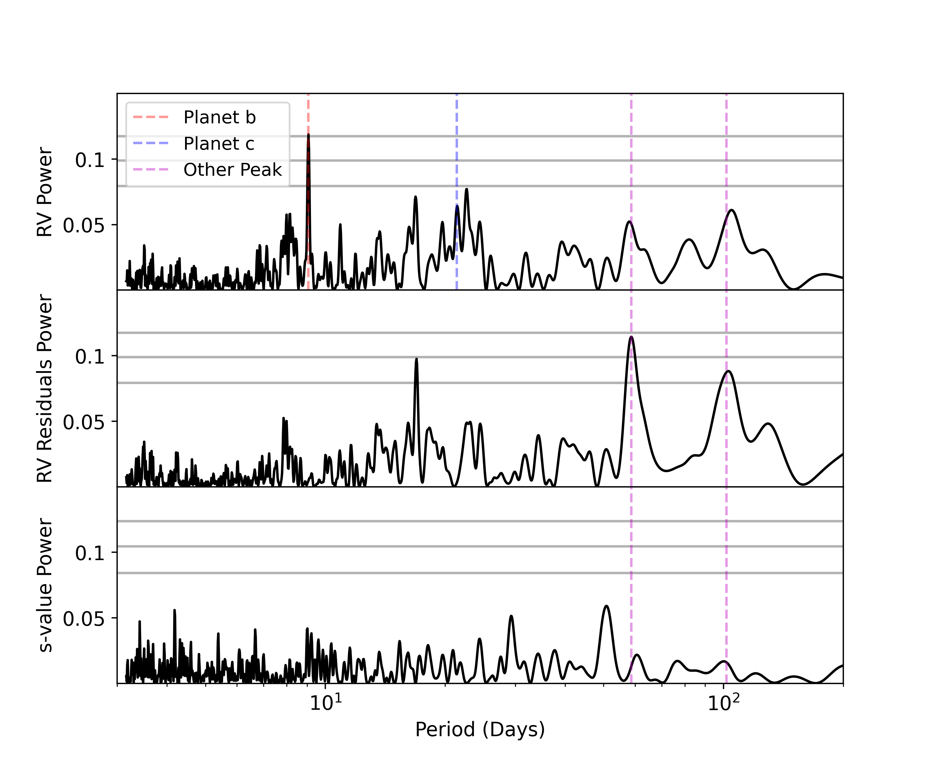
The photometry provides clear evidence for two planet candidates, whose presence we confirm with radial velocity followup. The residuals of a two-planet fit, however, show substantial structure. Because the HIRES and APF points in the residuals show similar behavior to each other, instrumental effects are unlikely to be the cause. This suggested that there was something still unaccounted for in our model, which could be a third planet. To test this, we generated a Lomb-Scargle periodogram of the radial velocity residuals from our two-planet fit (Figure 9). There are two primary visible peaks at longer periods, at 59 and 102 days. Because the peaks in the periodograms of the radial velocity residuals and s-values (activity indicators) do not correspond to each other, we consider it unlikely that this signal is caused by stellar activity. The lack of significant periodicity in the S-values suggests no motivation to adopt a Gaussian Process model for our data, consistent with our low value of R’HK. We have also performed an independent analysis (Section 3.2) to identify the stellar rotation period, arriving at the conclusion that this period is roughly 30-35 days, and therefore inconsistent with both of the longer-period RV periodogram peaks.
As a method of examining the significance of these peaks, we perform a bootstrap analysis. In this analysis we repeatedly resample our entire RV dataset with replacement, calculate the power at the locations in period space where the peak is highest in our true dataset, and repeat this 10000 times. Selecting a p value of 0.05, we are unable to reject the null hypothesis for either signal. Therefore, in this paper we have adopted the two-planet model, as the evidence for a third planet does not rise to the level of statistical significance we require. Important to note, however, is that this choice does not substantially impact the mass precision of our two confirmed planets, and the resulting masses are consistent to each other to 1- for both models. Further radial velocity monitoring or photometric followup could provide clarity as to the source of this additional signal.
| Nplanets | () | () | () |
|---|---|---|---|
| 2 | n/a | ||
| 3 ( d) | |||
| 3 ( d) |
The mass values for planets b and c for different possible models, as well as the for a possible third planet where relevant. Note that the masses for the two transiting planets are consistent within 1 no matter which model is selected.
6 Discussion
6.1 Examining Plausible Compositions
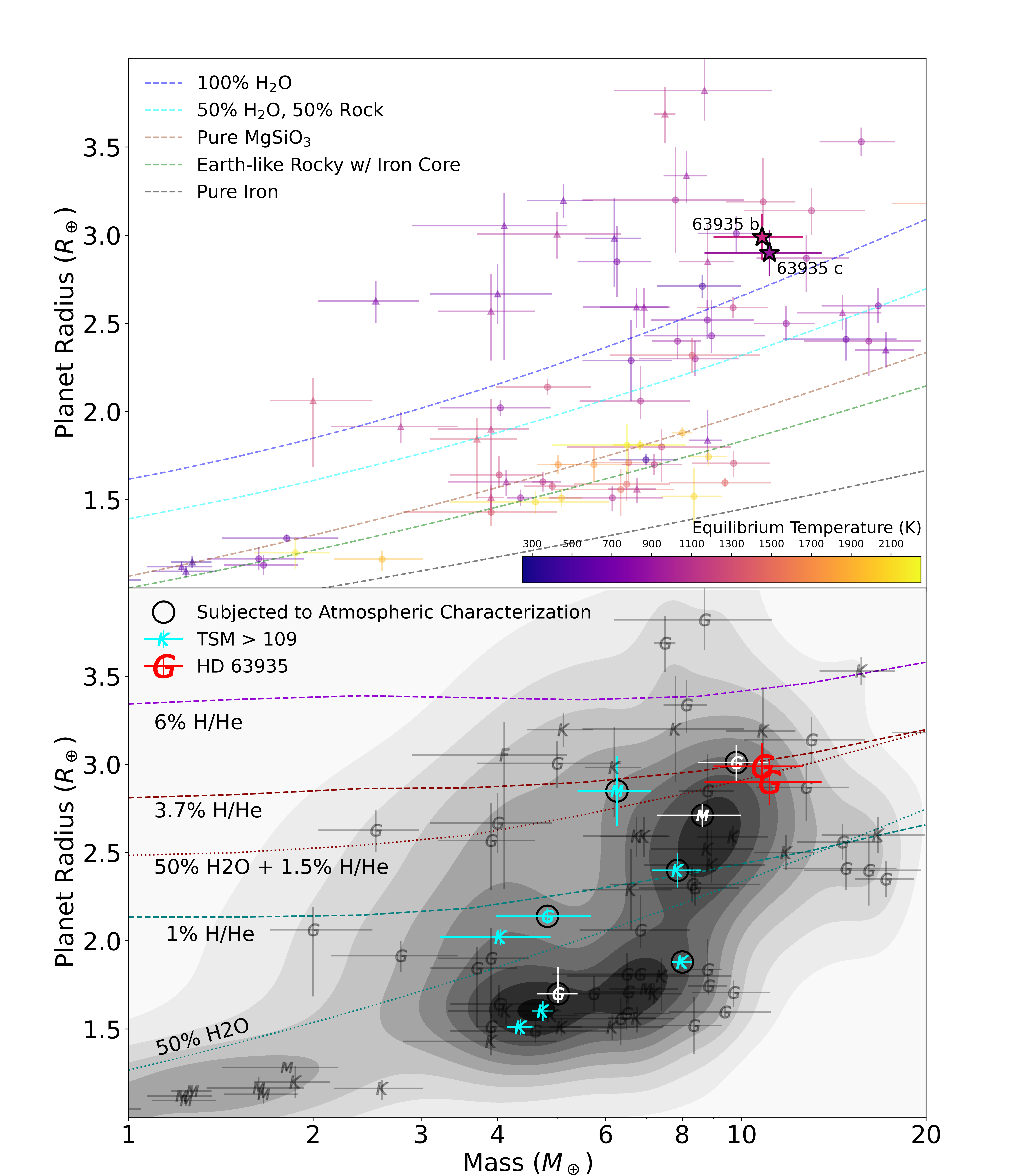
In order to better understand this planetary system, we investigated a range of possible compositions based on the planets’ bulk density and corresponding positions in mass-radius space. This is of particular interest given the substantial degeneracies in composition that exist for planets in this radius range, primarily between ice/volatile dominated planets and rock-dominated interiors with substantial H/He envelopes (Lopez & Fortney, 2014). To do this, we used the public tool smint888https://github.com/cpiaulet/smint (Piaulet et al., 2021), developed by Caroline Piaulet, which utilizes the models of Lopez & Fortney (2014) and Zeng et al. (2016) to do a Markov Chain Monte Carlo exploration of the posterior space of planetary interior compositions based on their mass, radius, age, and insolation flux. We use 25 MCMC walkers and 10000 steps for each in this analysis. Our results from smint are that HD 63935 b and c have % and % mass in H/He, respectively. Both planets could have cores that are intermediate between ice-dominated and rock-dominated. However, neither planet is sufficiently dense to be a pure “water world”; in other words, both are expected to have substantial (few percent mass) H/He envelopes. The compositional degeneracies that exist in this part of parameter space are one of the reasons that the sub-Neptune sized planets are so compelling for atmospheric characterization. Study of these planets’ atmospheres can potentially reveal more about their composition, which in turn can contribute to our understanding of how these planets form and why no analogs exist in our own solar system.
6.2 Nearly Twins: How Does HD 63935 Fit in the “Peas in a Pod” Structure?
Weiss et al. (2018) identified the phenomenon of Kepler planets in multi-planet systems being more likely to be similar to each other than drawn from a random distribution. They refer to this as “peas in a pod”. The two confirmed planets in the HD 63935 system appear to be in line with this trend, as both planets have masses and radii that are consistent to each other within one sigma. Higher precision measurements have the potential to distinguish differences between the two planets. In particular, if planet c is discovered to be higher density (as nominally appears to be the case, though the difference is not presently statistically significant), this would be interesting, because Weiss & Marcy (2014) note that the larger and lower density planet tends to be the exterior in their sample. They suggest that this result could be explained by photoevaporation. In this case, however, the nominally denser planet is the cooler and less-irradiated one, implying that a different explanation is required. We calculate the parameter described by Fossati et al. (2017), which estimates whether atmospheric erosion is relevant for a given planet. at T and at T (Fig 4 in Fossati et al. (2017)) are the relevant regions of atmospheric erosion for G star hosts. The respective values for HD 63935 b and c are 30 and 42, suggesting that neither planet is likely to experience significant atmospheric Jeans escape. In the absence of atmospheric loss, Zeng et al. (2019) propose that denser outer planets could be explained via impacts of ice-rich planetesimals (see also Marcus et al., 2009).
Also potentially of interest is the differing equilibrium temperatures of these planets (911K and 684K for b and c, respectively). Given their otherwise similar properties, they could serve as an experimental testing ground for the role of insolation on planetary composition and nature. As we describe in more detail in the following section, planets cooler than 1000K are likely to have decreasing spectral feature amplitude in transmission spectra as a result of increased haze formation (Gao et al., 2020). Observation of such a phenomenon in the HD 63935 system could be used as further evidence for this trend and of particular significance because the planets orbit the same star (eliminating a possible confounding variable).
6.3 Assessing Atmospheric Observability
As described above in Section 2, we identified HD 63935 b as the best target for atmospheric characterization followup in its region of parameter space (between 2.6 and 4 Earth radii, between 10 and 100 times Earth insolation flux, and stellar effective temperatures between 5200 and 6500K). The TSM value for HD 63935 b, incorporating our measured mass, is 108.8 35.8. In addition to its uniqueness within our algorithm’s defined parameter space bins, planet b is also of interest as a tool to probe the radius cliff, which refers to the apparent drop-off in planet occurrence rate above . In Figure 10, we identify planets with TSM values equal to or greater than that of HD 63935 b, and find that only one (HD 191939 b, Lubin et. al. (submitted)) falls on the radius cliff. The physical causes of the radius cliff are hypothesized to be related to atmospheric sequestration (Kite et al., 2019), signs of which may be visible in an atmosphere, further enhancing the target’s desirability for characterization. Note also that of the planets in that figure, four (HD 219134 b, HD 219134 c, 55 Cnc e, and Mensae c) have host star magnitudes that saturate JWST , meaning they are not suitable targets for transmission spectroscopy with JWST .
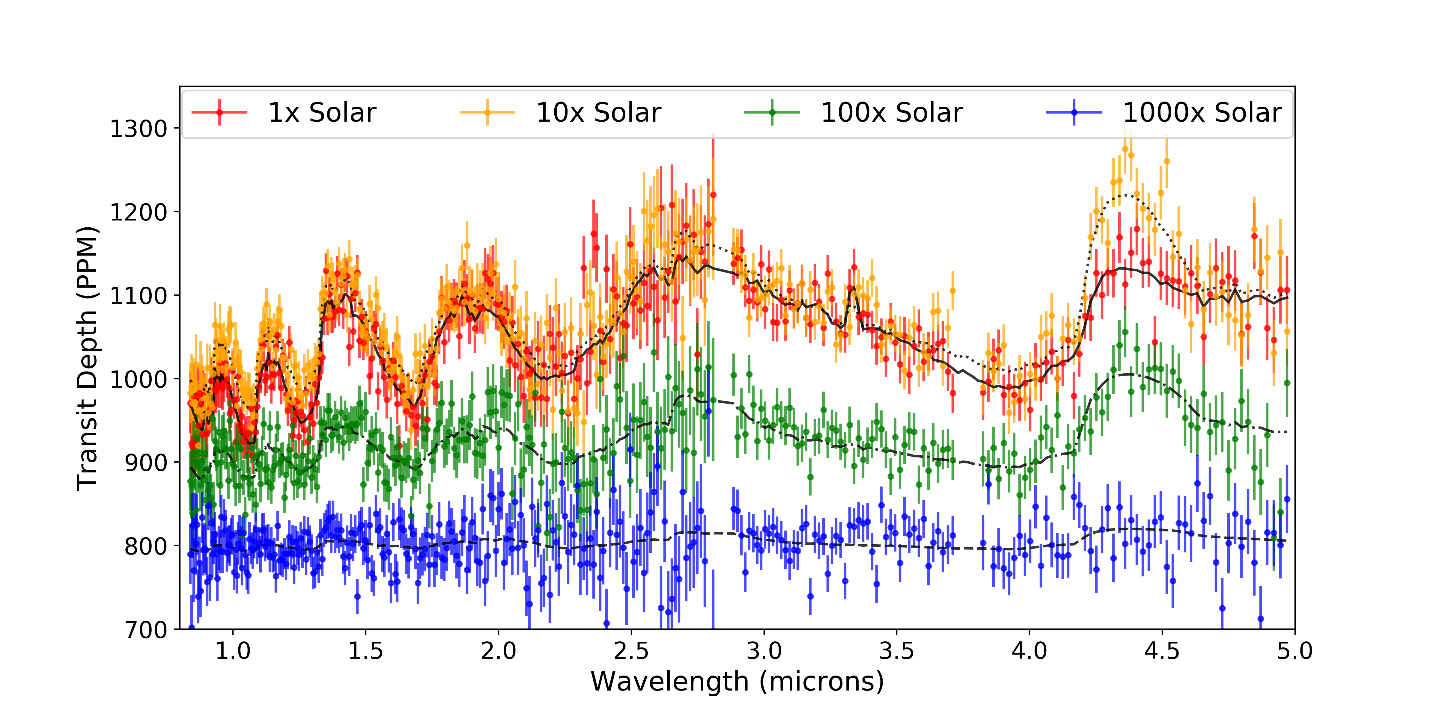
To validate the observability of HD 63935 b, we simulated planetary transmission spectra using CHIMERA (Line et al., 2012, 2013, 2014), then simulated transit observations of the planets using PandEXO (Batalha et al., 2017). A sample of our simulations (cloud-free cases only) are shown in Figure 11.
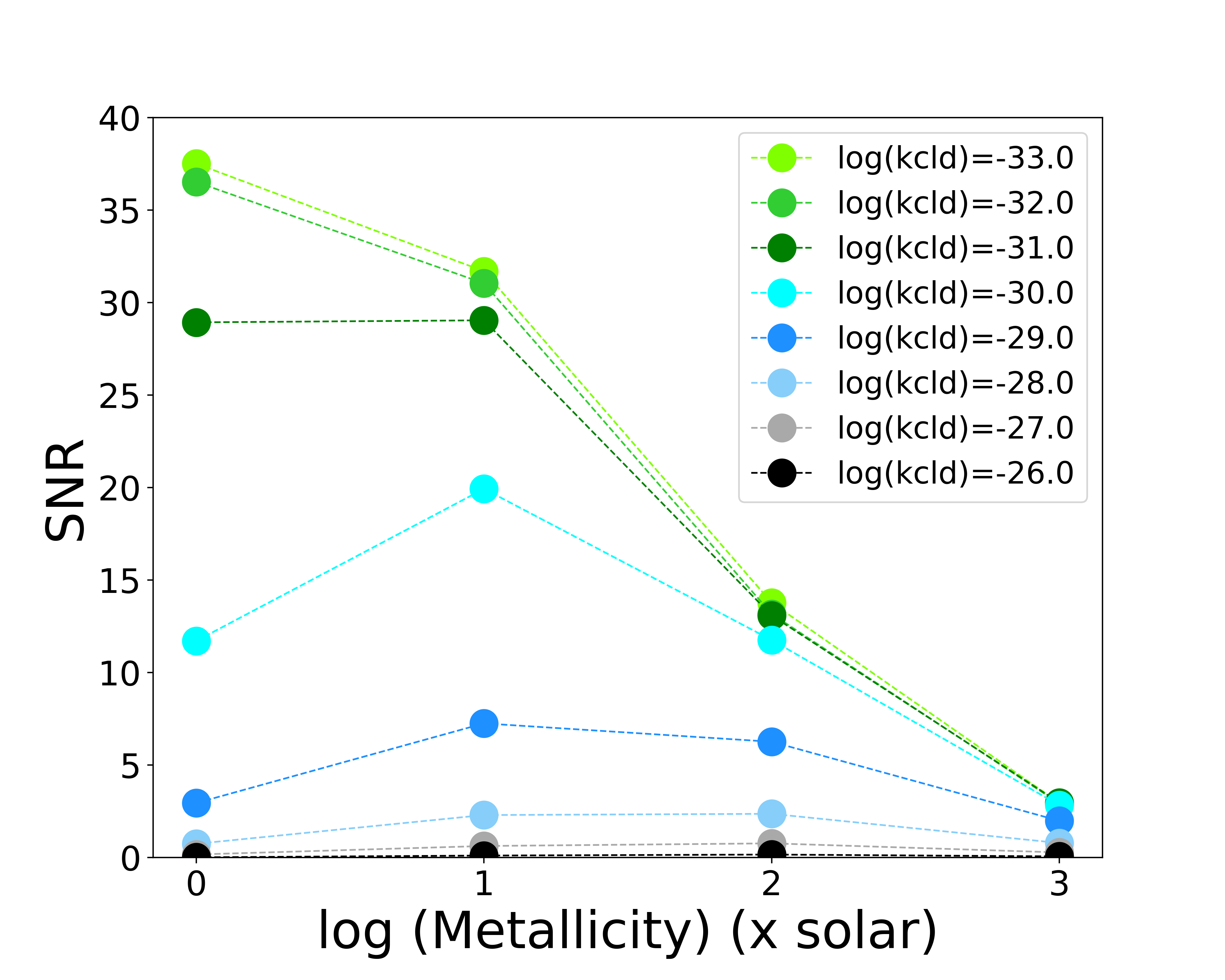
The results for planet b support our selection of the planet as one with an exceptionally high potential for atmospheric characterization. We simulated a range of metallicities and cloud opacities, then calculated the SNR of the water feature at 1.5m. We did this by simulating the spectrum 1000 times, determining the equivalent width of the feature in each, and finding the standard deviation of the resulting distribution. Our results are displayed in Figure 12. We emphasize that this is a conservative estimate of the quality of atmospheric spectra, but that even with middlingly-optimistic assumptions about metallicity and cloudiness, an observation of a single transit with JWST can produce useful spectra of this planet, and more observations would of course produce correspondingly more precise spectra.
Additionally, there is reason to expect that the atmosphere of HD 63935 b will have high-amplitude atmospheric features in its transmission spectrum. Although cloud formation in exoplanetary atmospheres is not fully understood, extensive modelling and analysis of existing transmission spectra have been done to attempt to understand which atmospheres will be dominated by clouds or hazes. Most recently, Gao et al. (2020) used an aerosol microphysics model to predict the dominant opacity sources in giant exoplanet transmission spectra. Their results suggest that the height of spectral features (specifically the 1.4 water band) increases with increasing temperature until 950 K, with opacity in this temperature regime dominated by high-altitude photochemical hazes derived from hydrocarbons. Above 950K, silicate condensate clouds become the dominant opacity source. These clouds rise higher into the atmosphere as temperature increases, resulting in reduced spectral feature amplitude with increasing temperature from 950 until 1800K. These predictions are highly relevant to this work, as HD 63935 b sits quite close to the critical equilibrium temperature of 950K which we expect to be a local maximum of feature amplitude.
This prediction is also in line with earlier work by Crossfield & Kreidberg (2017), which analyzed the published transmission spectra of exclusively Neptune-sized exoplanets and found a positive correlation between feature height and equilibrium temperature in their domain of 500-1100K. Taken together, these results suggest that HD 63935 b is in a region of parameter space that is maximally likely to produce observable spectral features. Combined with its other desirable qualities as an atmospheric target (bright host star, large TSM value), it is clear that HD 63935 b has exceptional promise as a target for atmospheric characterization.
Finally, we note that HD 63935 is quite sun-like (M, [Fe/H] = 0.07 0.06), making characterization of its planetary system of additional interest for comparative planetology with our own solar system. We also emphasize that only one sub-Neptune planet around such a similar star has a published atmospheric characterization study (HD 3167 c Mikal-Evans et al., 2020). Combined with other such planets with G-type host stars being discovered by TESS, it could form part of a robust population study.
7 Conclusions
We have described the discovery of two planets around the bright G star HD 63935.
-
•
HD 63935 b and c have periods and days, radii and , and masses and .
-
•
Both confirmed planets have a radius higher than the median sub-Neptune and fall on the ”radius cliff”.
-
•
Planet b is an outstanding target for transmission spectroscopy, being the best target in its parameter space niche and second-best among targets on the radius cliff, while planet c is also amenable to atmospheric characterization. This quality for followup is exceptionally enticing given the compositional degeneracies that exist in this region of parameter space, which could be broken with high-quality atmospheric characterization.
-
•
Atmospheric characterization of this system could provide valuable input to theories of planetary interiors, formation, and evolution, especially given that two planets similar in all observed properties except insolation flux is as close to a variable-controlled experimental setup as exoplanet astronomy typically comes.
HD 63935 b and c attest to the bright future of exoplanet astronomy and we expect this system to be an excellent test case for studying exoplanetary atmospheres in coming years.
Facilities Automated Planet Finder (Levy), HARPS-N (TNG), HIRES (Keck I), Las Cumbres Observatory Global Telescope (LCOGT), NIRC2 (Keck II), PHARO (Palomar), TESS
Software AstroImageJ (Collins et al., 2017), Astropy (Robitaille et al., 2013), batman (Kreidberg, 2015), emcee (Foreman-Mackey et al., 2013b), exoplanet and its dependencies (Foreman-Mackey et al., 2021; Agol et al., 2020; Kumar et al., 2019; Luger et al., 2019; Salvatier et al., 2016; Theano Development Team, 2016), isoclassify (Huber et al., 2017), juliet (Espinoza et al., 2019), Jupyter (Kluyver et al., 2016), kiauhoku (Claytor et al., 2020), matplotlib (Hunter, 2007), numpy (Harris et al., 2020), pandas (McKinney et al., 2010), Radvel (Fulton et al., 2018), smint (Piaulet et al., 2021), SpecMatch-Syn (Petigura et al., 2017) Transit Least Squares (Hippke & Heller, 2019)
8 Acknowledgments
We thank the anonymous referee for their helpful feedback that improved the quality of this work. We thank the time assignment committees of the University of California, the California Institute of Technology, NASA, and the University of Hawaii for supporting the TESS-Keck Survey with observing time at Keck Observatory and on the Automated Planet Finder. We thank NASA for funding associated with our Key Strategic Mission Support project. We gratefully acknowledge the efforts and dedication of the Keck Observatory staff for support of HIRES and remote observing. We recognize and acknowledge the cultural role and reverence that the summit of Maunakea has within the indigenous Hawaiian community. We are deeply grateful to have the opportunity to conduct observations from this mountain. We thank Ken and Gloria Levy, who supported the construction of the Levy Spectrometer on the Automated Planet Finder. We thank the University of California and Google for supporting Lick Observatory and the UCO staff for their dedicated work scheduling and operating the telescopes of Lick Observatory.
This paper is based on data collected by the TESS mission. Funding for the TESS mission is provided by NASA’s Science Mission Directorate. We acknowledge the use of public TESS data from pipelines at the TESS Science Office and at the TESS Science Processing Operations Center. This research has made use of the Exoplanet Follow-up Observation Program website, which is operated by the California Institute of Technology, under contract with the National Aeronautics and Space Administration under the Exoplanet Exploration Program. Resources supporting this work were provided by the NASA High-End Computing (HEC) Program through the NASA Advanced Supercomputing (NAS) Division at Ames Research Center for the production of the SPOC data products. This paper includes data collected by the TESS mission that are publicly available from the Mikulski Archive for Space Telescopes (MAST). This research has made use of the NASA Exoplanet Archive and Exoplanet Follow-up Observation Program website, which are operated by the California Institute of Technology, under contract with the National Aeronautics and Space Administration under the Exoplanet Exploration Program. Based on observations made with the Italian Telescopio Nazionale Galileo (TNG) operated on the island of La Palma by the Fundación Galileo Galilei of the INAF (Istituto Nazionale di Astrofisica) at the Spanish Observatorio del Roque de los Muchachos of the Instituto de Astrofisica de Canarias under programmes CAT19A_162 and CAT19A_96. This work has made use of data from the European Space Agency (ESA) mission Gaia (https://www.cosmos.esa.int/gaia), processed by the Gaia Data Processing and Analysis Consortium (DPAC, https://www.cosmos.esa.int/web/gaia/dpac/consortium). Funding for the DPAC has been provided by national institutions, in particular the institutions participating in the Gaia Multilateral Agreement. This work is partly supported by JSPS KAKENHI Grant Numbers JP17H04574 and JP18H05439, JST PRESTO Grant Number JPMJPR1775, and Grant-in-Aid for JSPS Fellows, Grant Number JP20J21872. This work makes use of observations from the LCOGT network.
D. D. acknowledges support from the TESS Guest Investigator Program grant 80NSSC19K1727 and NASA Exoplanet Research Program grant 18-2XRP18_2-0136. J.M.A.M. is supported by the National Science Foundation Graduate Research Fellowship Program under Grant No. DGE-1842400. J.M.A.M. acknowledges the LSSTC Data Science Fellowship Program, which is funded by LSSTC, NSF Cybertraining Grant No. 1829740, the Brinson Foundation, and the Moore Foundation; his participation in the program has benefited this work. M.R.K. is supported by the NSF Graduate Research Fellowship, grant No. DGE 1339067. P.D. acknowledges support from a National Science Foundation Astronomy and Astrophysics Postdoctoral Fellowship under award AST-1903811.
References
- Agol et al. (2020) Agol, E., Luger, R., & Foreman-Mackey, D. 2020, AJ, 159, 123
- Baranne et al. (1996) Baranne, A., Queloz, D., Mayor, M., et al. 1996, A&AS, 119, 373
- Batalha et al. (2019) Batalha, N. E., Lewis, T., Fortney, J. J., et al. 2019, arXiv e-prints, arXiv:1910.00076
- Batalha et al. (2017) Batalha, N. E., Mandell, A., Pontoppidan, K., et al. 2017, Publications of the Astronomical Society of the Pacific, 129, 064501
- Batalha et al. (2013) Batalha, N. M., Rowe, J. F., Bryson, S. T., et al. 2013, The Astrophysical Journal Supplement Series, 204, 24
- Berger et al. (2020) Berger, T. A., Huber, D., van Saders, J. L., et al. 2020, The Gaia-Kepler Stellar Properties Catalog. I. Homogeneous Fundamental Properties for 186,301 Kepler Stars, , , arXiv:2001.07737
- Borucki et al. (2011) Borucki, W. J., Koch, D. G., Basri, G., et al. 2011, The Astrophysical Journal, 736, 19
- Brown et al. (2013) Brown, T. M., Baliber, N., Bianco, F. B., et al. 2013, Publications of the Astronomical Society of the Pacific, 125, 1031–1055
- Buchhave et al. (2012) Buchhave, L. A., Latham, D., Johansen, A., et al. 2012, Nature, 486, 375
- Buchner et al. (2014) Buchner, J., Georgakakis, A., Nandra, K., et al. 2014, Astronomy & Astrophysics, 564, A125
- Chen & Kipping (2016) Chen, J., & Kipping, D. 2016, The Astrophysical Journal, 834, 17
- Ciardi et al. (2015) Ciardi, D. R., Beichman, C. A., Horch, E. P., & Howell, S. B. 2015, The Astrophysical Journal, 805, 16
- Claytor et al. (2020) Claytor, Z. R., Saders, J. L. v., Santos, A. R. G., et al. 2020, The Astrophysical Journal, 888, 43
- Collaboration et al. (2020) Collaboration, G., Brown, A. G. A., Vallenari, A., et al. 2020, Gaia Early Data Release 3: Summary of the contents and survey properties, , , arXiv:2012.01533
- Collins et al. (2017) Collins, K. A., Kielkopf, J. F., Stassun, K. G., & Hessman, F. V. 2017, AJ, 153, 77
- Cosentino et al. (2012) Cosentino, R., Lovis, C., Pepe, F., et al. 2012, in Society of Photo-Optical Instrumentation Engineers (SPIE) Conference Series, Vol. 8446, Ground-based and Airborne Instrumentation for Astronomy IV, 84461V
- Cosentino et al. (2014) Cosentino, R., Lovis, C., Pepe, F., et al. 2014, in Society of Photo-Optical Instrumentation Engineers (SPIE) Conference Series, Vol. 9147, Ground-based and Airborne Instrumentation for Astronomy V, 91478C
- Crossfield & Kreidberg (2017) Crossfield, I. J. M., & Kreidberg, L. 2017, The Astronomical Journal, 154, 261
- Crossfield et al. (2016) Crossfield, I. J. M., Ciardi, D. R., Petigura, E. A., et al. 2016, ApJS, 226, 7
- Dai et al. (2020) Dai, F., Roy, A., Fulton, B., et al. 2020, The Astronomical Journal, 160, 193
- Dalba et al. (2020) Dalba, P. A., Gupta, A. F., Rodriguez, J. E., et al. 2020, The Astronomical Journal, 159, 241
- Dekany et al. (2013) Dekany, R., Roberts, J., Burruss, R., et al. 2013, The Astrophysical Journal, 776, 130
- Espinoza et al. (2019) Espinoza, N., Kossakowski, D., & Brahm, R. 2019, MNRAS, 490, 2262
- Fűrész (2008) Fűrész, G. 2008, PhD thesis, University of Szeged, Hungary
- Foreman-Mackey et al. (2013a) Foreman-Mackey, D., Hogg, D. W., Lang, D., & Goodman, J. 2013a, PASP, 125, 306
- Foreman-Mackey et al. (2013b) —. 2013b, PASP, 125, 306
- Foreman-Mackey et al. (2021) Foreman-Mackey, D., Savel, A., Luger, R., et al. 2021, exoplanet-dev/exoplanet v0.4.4, , , doi:10.5281/zenodo.1998447
- Fossati et al. (2017) Fossati, L., Erkaev, N. V., Lammer, H., et al. 2017, Astronomy & Astrophysics, 598, A90
- Fukui et al. (2011) Fukui, A., Narita, N., Tristram, P. J., et al. 2011, Publications of the Astronomical Society of Japan, 63, 287–300
- Fulton et al. (2018) Fulton, B. J., Petigura, E. A., Blunt, S., & Sinukoff, E. 2018, PASP, 130, 044504
- Fulton et al. (2017) Fulton, B. J., Petigura, E. A., Howard, A. W., et al. 2017, AJ, 154, 109
- Furlan et al. (2017) Furlan, E., Ciardi, D. R., Everett, M. E., et al. 2017, The Astronomical Journal, 153, 71
- Gaia Collaboration et al. (2018) Gaia Collaboration, Brown, A. G. A., Vallenari, A., et al. 2018, ArXiv e-prints, arXiv:1804.09365
- Gandolfi et al. (2018) Gandolfi, D., Barragán, O., Livingston, J. H., et al. 2018, Astronomy & Astrophysics, 619, L10
- Gao et al. (2020) Gao, P., Thorngren, D. P., Lee, G. K. H., et al. 2020, Nature Astronomy, 4, 951–956
- Guerrero et al. (2021) Guerrero, N. M., Seager, S., Huang, C. X., et al. 2021, The TESS Objects of Interest Catalog from the TESS Prime Mission, , , arXiv:2103.12538
- Harris et al. (2020) Harris, C. R., Millman, K. J., van der Walt, S. J., et al. 2020, Nature, 585, 357
- Hayward et al. (2001) Hayward, T. L., Brandl, B., Pirger, B., et al. 2001, Publications of the Astronomical Society of the Pacific, 113, 105
- Hippke & Heller (2019) Hippke, M., & Heller, R. 2019, A&A, 623, A39
- Howard et al. (2010) Howard, A. W., Johnson, J. A., Marcy, G. W., et al. 2010, ApJ, 721, 1467
- Howard et al. (2012) Howard, A. W., Marcy, G. W., Bryson, S. T., et al. 2012, ApJS, 201, 15
- Huber et al. (2017) Huber, D., Zinn, J., Bojsen-Hansen, M., et al. 2017, The Astrophysical Journal, 844, 102
- Hunter (2007) Hunter, J. D. 2007, Computing in Science & Engineering, 9, 90
- Jenkins (2002) Jenkins, J. M. 2002, The Astrophysical Journal, 575, 493
- Jenkins et al. (2010) Jenkins, J. M., Caldwell, D. A., Chandrasekaran, H., et al. 2010, ApJ, 713, L87
- Jenkins et al. (2016) Jenkins, J. M., Twicken, J. D., McCauliff, S., et al. 2016, in Software and Cyberinfrastructure for Astronomy IV, ed. G. Chiozzi & J. C. Guzman, Vol. 9913, International Society for Optics and Photonics (SPIE), 1232 – 1251
- Jensen (2013) Jensen, E. 2013, Tapir: A web interface for transit/eclipse observability, Astrophysics Source Code Library, , , ascl:1306.007
- Kempton et al. (2018) Kempton, E. M. R., Bean, J. L., Louie, D. R., et al. 2018, PASP, 130, 114401
- Kipping (2013) Kipping, D. M. 2013, Monthly Notices of the Royal Astronomical Society, 435, 2152–2160
- Kite et al. (2019) Kite, E. S., Jr., B. F., Schaefer, L., & Ford, E. B. 2019, The Astrophysical Journal, 887, L33
- Kluyver et al. (2016) Kluyver, T., Ragan-Kelley, B., Pérez, F., et al. 2016, in Positioning and Power in Academic Publishing: Players, Agents and Agendas, ed. F. Loizides & B. Scmidt (IOS Press), 87–90
- Kreidberg (2015) Kreidberg, L. 2015, PASP, 127, 1161
- Kruse et al. (2019) Kruse, E., Agol, E., Luger, R., & Foreman-Mackey, D. 2019, The Astrophysical Journal Supplement Series, 244, 11
- Kumar et al. (2019) Kumar, R., Carroll, C., Hartikainen, A., & Martin, O. A. 2019, The Journal of Open Source Software, doi:10.21105/joss.01143
- Kurucz (1993) Kurucz, R. L. 1993, SYNTHE spectrum synthesis programs and line data
- Li et al. (2019) Li, J., Tenenbaum, P., Twicken, J. D., et al. 2019, Publications of the Astronomical Society of the Pacific, 131, 024506
- Line et al. (2014) Line, M. R., Knutson, H., Wolf, A. S., & Yung, Y. L. 2014, The Astrophysical Journal, 783, 70
- Line et al. (2012) Line, M. R., Zhang, X., Vasisht, G., et al. 2012, ApJ, 749, 93
- Line et al. (2013) Line, M. R., Wolf, A. S., Zhang, X., et al. 2013, The Astrophysical Journal, 775, 137
- Lopez & Fortney (2014) Lopez, E. D., & Fortney, J. J. 2014, ApJ, 792, 1
- Luger et al. (2019) Luger, R., Agol, E., Foreman-Mackey, D., et al. 2019, AJ, 157, 64
- Lund (Submitted) Lund, M. B. Submitted
- Mann et al. (2020) Mann, A. W., Johnson, M. C., Vanderburg, A., et al. 2020, The Astronomical Journal, 160, 179
- Marcus et al. (2009) Marcus, R. A., Stewart, S. T., Sasselov, D., & Hernquist, L. 2009, The Astrophysical Journal, 700, L118–L122
- Martin & Livio (2015) Martin, R. G., & Livio, M. 2015, The Astrophysical Journal, 810, 105
- McCully et al. (2018) McCully, C., Volgenau, N. H., Harbeck, D.-R., et al. 2018, in Society of Photo-Optical Instrumentation Engineers (SPIE) Conference Series, Vol. 10707, Proc. SPIE, 107070K
- McKinney et al. (2010) McKinney, W., et al. 2010, in Proceedings of the 9th Python in Science Conference, Vol. 445, Austin, TX, 51–56
- Mikal-Evans et al. (2020) Mikal-Evans, T., Crossfield, I. J. M., Benneke, B., et al. 2020, Transmission spectroscopy for the warm sub-Neptune HD3167c: evidence for molecular absorption and a possible high metallicity atmosphere, , , arXiv:2011.03470
- Mink (2011) Mink, D. J. 2011, in Astronomical Society of the Pacific Conference Series, Vol. 442, Astronomical Data Analysis Software and Systems XX, ed. I. N. Evans, A. Accomazzi, D. J. Mink, & A. H. Rots, 305
- Morris et al. (2020) Morris, R. L., Twicken, J. D., Smith, J. C., et al. 2020, Kepler Data Processing Handbook
- Narita et al. (2015) Narita, N., Fukui, A., Kusakabe, N., et al. 2015, Journal of Astronomical Telescopes, Instruments, and Systems, 1, 045001
- Owen & Wu (2017) Owen, J. E., & Wu, Y. 2017, The Astrophysical Journal, 847, 29
- Paunzen (2015) Paunzen, E. 2015, Astronomy & Astrophysics, 580, A23
- Petigura et al. (2017) Petigura, E. A., Howard, A. W., Marcy, G. W., et al. 2017, The Astronomical Journal, 154, 107
- Piaulet et al. (2021) Piaulet, C., Benneke, B., Rubenzahl, R. A., et al. 2021, The Astronomical Journal, 161, 70
- Plavchan et al. (2015) Plavchan, P., Latham, D., Gaudi, S., et al. 2015, Radial Velocity Prospects Current and Future: A White Paper Report prepared by the Study Analysis Group 8 for the Exoplanet Program Analysis Group (ExoPAG), , , arXiv:1503.01770
- Prusti et al. (2016) Prusti, T., de Bruijne, J. H. J., Brown, A. G. A., et al. 2016, Astronomy & Astrophysics, 595, A1
- Quirrenbach & Consortium (2020) Quirrenbach, A., & Consortium, C. 2020, in Ground-based and Airborne Instrumentation for Astronomy VIII, ed. C. J. Evans, J. J. Bryant, & K. Motohara, Vol. 11447, International Society for Optics and Photonics (SPIE), 701 – 711
- Radovan et al. (2010) Radovan, M. V., Cabak, G. F., Laiterman, L. H., Lockwood, C. T., & Vogt, S. S. 2010, in Society of Photo-Optical Instrumentation Engineers (SPIE) Conference Series, Vol. 7735, Ground-based and Airborne Instrumentation for Astronomy III, 77354K
- Ricker et al. (2014) Ricker, G. R., Winn, J. N., Vanderspek, R., et al. 2014, Journal of Astronomical Telescopes, Instruments, and Systems, 1, 014003
- Robitaille et al. (2013) Robitaille, T. P., Tollerud, E. J., Greenfield, P., et al. 2013, Astronomy & Astrophysics, 558, A33
- Rogers (2015) Rogers, L. A. 2015, The Astrophysical Journal, 801, 41
- Rubenzahl et al. (2021) Rubenzahl, R. A., Dai, F., Howard, A. W., et al. 2021, The Astronomical Journal, 161, 119
- Salvatier et al. (2016) Salvatier, J., Wiecki, T. V., & Fonnesbeck, C. 2016, PeerJ Computer Science, 2, e55
- Schlegel et al. (1998) Schlegel, D. J., Finkbeiner, D. P., & Davis, M. 1998, ApJ, 500, 525
- Seifahrt et al. (2018) Seifahrt, A., Stürmer, J., Bean, J. L., & Schwab, C. 2018, MAROON-X: A Radial Velocity Spectrograph for the Gemini Observatory, , , arXiv:1805.09276
- Siverd et al. (2018) Siverd, R. J., Brown, T. M., Barnes, S., et al. 2018, in Ground-based and Airborne Instrumentation for Astronomy VII, ed. C. J. Evans, L. Simard, & H. Takami, Vol. 10702, International Society for Optics and Photonics (SPIE), 1918 – 1929
- Smith et al. (2012) Smith, J. C., Stumpe, M. C., Cleve, J. E. V., et al. 2012, Publications of the Astronomical Society of the Pacific, 124, 1000
- Stassun et al. (2017) Stassun, K. G., Collins, K. A., & Gaudi, B. S. 2017, AJ, 153, 136
- Stassun et al. (2018) Stassun, K. G., Corsaro, E., Pepper, J. A., & Gaudi, B. S. 2018, AJ, 155, 22
- Stassun & Torres (2016) Stassun, K. G., & Torres, G. 2016, AJ, 152, 180
- Stumpe et al. (2014) Stumpe, M. C., Smith, J. C., Catanzarite, J. H., et al. 2014, 126, 100
- Stumpe et al. (2012) Stumpe, M. C., Smith, J. C., Cleve, J. E. V., et al. 2012, Publications of the Astronomical Society of the Pacific, 124, 985
- Tayar et al. (2020) Tayar, J., Claytor, Z. R., Huber, D., & van Saders, J. 2020, A Guide to Realistic Uncertainties on Fundamental Properties of Solar-Type Exoplanet Host Stars, , , arXiv:2012.07957
- Theano Development Team (2016) Theano Development Team. 2016, arXiv e-prints, abs/1605.02688
- Thompson et al. (2018) Thompson, S. E., Coughlin, J. L., Hoffman, K., et al. 2018, The Astrophysical Journal Supplement Series, 235, 38
- Torres et al. (2010) Torres, G., Andersen, J., & Giménez, A. 2010, A&A Rev., 18, 67
- Twicken et al. (2010) Twicken, J. D., Clarke, B. D., Bryson, S. T., et al. 2010, in Software and Cyberinfrastructure for Astronomy, ed. N. M. Radziwill & A. Bridger, Vol. 7740, International Society for Optics and Photonics (SPIE), 749 – 760
- Twicken et al. (2018) Twicken, J. D., Catanzarite, J. H., Clarke, B. D., et al. 2018, Publications of the Astronomical Society of the Pacific, 130, 064502
- van Saders et al. (2016) van Saders, J. L., Ceillier, T., Metcalfe, T. S., et al. 2016, Nature, 529, 181–184
- van Saders & Pinsonneault (2013) van Saders, J. L., & Pinsonneault, M. H. 2013, The Astrophysical Journal, 776, 67
- Vogt et al. (1994) Vogt, S. S., Allen, S. L., Bigelow, B. C., et al. 1994, in Proc. SPIE, Vol. 2198, Instrumentation in Astronomy VIII, ed. D. L. Crawford & E. R. Craine, 362
- Vogt et al. (2014) Vogt, S. S., Radovan, M., Kibrick, R., et al. 2014, Publications of the Astronomical Society of the Pacific, 126, 359–379
- Weiss & Marcy (2014) Weiss, L. M., & Marcy, G. W. 2014, ApJ, 783, L6
- Weiss et al. (2018) Weiss, L. M., Marcy, G. W., Petigura, E. A., et al. 2018, The Astronomical Journal, 155, 48
- Weiss et al. (2020) Weiss, L. M., Dai, F., Huber, D., et al. 2020, The TESS-Keck Survey II: Masses of Three Sub-Neptunes Transiting the Galactic Thick-Disk Star TOI-561, , , arXiv:2009.03071
- Weiss et al. (2021) —. 2021, The Astronomical Journal, 161, 56
- Wizinowich et al. (2000) Wizinowich, P., Acton, D. S., Shelton, C., et al. 2000, Publications of the Astronomical Society of the Pacific, 112, 315
- Wolfgang et al. (2016) Wolfgang, A., Rogers, L. A., & Ford, E. B. 2016, The Astrophysical Journal, 825, 19
- Zechmeister et al. (2018) Zechmeister, M., Reiners, A., Amado, P. J., et al. 2018, A&A, 609, A12
- Zeng et al. (2016) Zeng, L., Sasselov, D. D., & Jacobsen, S. B. 2016, ApJ, 819, 127
- Zeng et al. (2019) Zeng, L., Jacobsen, S. B., Sasselov, D. D., et al. 2019, Proceedings of the National Academy of Sciences, 116, 9723