The Belle II Collaboration
Test of lepton flavor universality with measurements of and using semileptonic tagging at the Belle II experiment
Abstract
We report measurements of the ratios of branching fractions , where denotes either an electron or a muon. These ratios test the universality of the charged-current weak interaction. The results are based on a data sample collected with the Belle II detector at the SuperKEKB collider, which operates at a center-of-mass energy corresponding to the resonance, just above the threshold for production. Signal candidates are reconstructed by selecting events in which the companion meson from the decay is identified in semileptonic modes. The lepton is reconstructed via its leptonic decays. We obtain and , which are consistent with world average values. Accounting for the correlation between them, these values differ from the Standard Model expectation by a collective significance of standard deviations.
I Introduction
A fundamental property of the Standard Model (SM) of particle physics is the universality of the electroweak gauge couplings to the three fermion generations. In the lepton sector, this universality results in an accidental symmetry of the lepton flavors that is only broken by the Higgs-Yukawa interaction. One key consequence is that physical processes involving charged leptons feature lepton flavor universality (LFU), an approximate symmetry of lepton flavor among physical observables, only broken by charged lepton mass terms emerging from the non-zero vacuum expectation value of the Higgs field. An observation of lepton flavor universality violation would therefore be a clear signature of physics beyond the SM [1].
In this paper, we test LFU using semitauonic decays by measuring the ratios,111Charge conjugation is implied throughout this paper.
| (1) |
with and denoting either or . The first equality follows from the assumption of isospin symmetry. Predictions of these ratios are independent of the magnitude of the Cabibbo-Kobayashi-Maskawa (CKM) matrix element and, to some extent, of the parameterization of hadronic matrix elements, reaching a precision of 1–2% [2, 3, 4, 5, 6, 7, 8, 9, 10]. Experimentally, measurements of the ratios in Eq. 1 are preferred to measurements of absolute branching fractions, as efficiency-related systematic uncertainties largely cancel. Furthermore, the simultaneous measurement of both and is useful, as decays are an important background in the reconstruction of decays.
Several experiments previously reported measurements of these or similar ratios [11, 12, 13, 14, 15, 16, 17, 18, 19, 20, 21, 22]. Belle II reported [23] and the inclusive ratio [24]. A combination of these measurements is reported in Ref. [25] and achieves a precision of 8% for and 4% for , with values of and . Both exceed the SM expectations of and [2, 3, 4, 5, 6, 7, 8, 9, 10] with a significance of 3.1 standard deviations.
In this analysis, we study pairs produced in decays. One or meson is reconstructed in a semileptonic decay using the hierarchical reconstruction algorithm from Ref. [26], referred to as . This is then combined with an oppositely flavored semitauonic or semileptonic decay candidate, which we define as . The selected events are independent of those analyzed in Refs. [24, 23], as the latter relied on the reconstruction of hadronically decaying mesons. The analysis of pairs is deferred to future work, as the reconstruction of the isospin-conjugate signal decays necessitates the efficient identification of decays, which suffer from an increased combinatorial background.
We reconstruct signal candidates from the and final states (with ), which can originate from either semitauonic decays ( with ) or semileptonic decays (). These processes differ in the number of neutrinos and are thus distinguishable through kinematic properties. Since both processes produce the same visible final state in the detector, several experimental systematic uncertainties cancel in the measurement of their ratio.
We distinguish candidates originating from semitauonic, semileptonic, and background sources using multivariate classifiers trained on the kinematic properties of both the and candidates. A binned maximum likelihood fit is then performed to measure the relative contribution from each source, allowing a direct determination of .
The remainder of this paper is structured as follows: Sections II and III provide an overview of the Belle II detector, the analyzed data set, and the simulated samples. Section IV summarizes the tag and signal reconstruction, while Section V describes the employed multivariate selection. Section VI details the fitting procedure, and Section VII discusses the systematic uncertainties affecting the measurement. Section VIII presents our findings and consisitency checks, and Section IX provides our conclusions.
II Belle II detector and data set
The analysis uses Belle II data collected at SuperKEKB [27] from 2019 to 2022 at a center-of-mass energy of 10.58 GeV,222Natural units () are used throughout this paper. corresponding to the resonance, having an integrated luminosity of 365 . The sample contains an estimated events. Additionally, 42.3 fb-1 of off-resonance data at 10.52 GeV is used to study () background.
The Belle II detector [28] is an upgraded version of Belle [29] with enhanced particle reconstruction and identification. Its subdetectors are arranged cylindrically around the interaction point (IP), which is enclosed by a beryllium beam pipe. The pixel detector (PXD) consists of two layers, with the first fully instrumented and the second partially completed. The PXD is surrounded by a four-layer double-sided silicon-strip detector (SVD), and both detectors are used to reconstruct decay vertices with high precision. Surrounding these detectors is the central drift chamber (CDC), which provides three-dimensional tracking and specific ionization () measurements.
Outside the CDC, the time-of-propagation (TOP) and aerogel ring-imaging Cherenkov (ARICH) detectors provide particle identification in the barrel and forward endcap regions, respectively.
The electromagnetic calorimeter (ECL), consisting of a barrel and annular endcaps, is located outside the TOP and within a superconducting solenoid. The and muon detector (KLM), situated outside the solenoid, is composed of iron plates interleaved with active detector elements.
Particle candidates are constructed and identified using the information from various detector systems.
Charged particle candidates (tracks) are reconstructed by the vertex and tracking systems, and identified based on information from the outer detectors. In particular, muons with sufficiently high momentum will traverse the KLM, while other charged particles are absorbed. In contrast, electrons deposit nearly all of their energy in the ECL.
Photon candidates consist of ECL clusters that are not consistent with extrapolations of charged tracks. Minimum energy selections are necessary to reject clusters from beam-induced background photons.
III Simulation
Monte Carlo (MC) samples are used to determine reconstruction efficiencies and acceptance effects as well as to estimate background contamination and to train multivariate classifiers. The decays are simulated using the EvtGen generator [30]. The simulation of continuum processes is carried out with KKMC [31] and PYTHIA8 [32]. Electromagnetic final-state radiation is simulated using PHOTOS [33] for all charged final-state particles. Interactions of particles with the detector are simulated using GEANT4 [34]. The simulated samples contain the equivalent of 2.8 ab-1 of and continuum processes. The events are simulated with equal fractions of neutral and charged mesons. An additional sample of decays with is used, corresponding to an effective sample size of ab-1.
The signal decays and are modeled using the form factors from Ref. [6], with parameter values obtained from a fit to the measurements in Refs. [35, 36]. To incorporate this form factor model into the Monte Carlo simulation, the HAMMER software package [37] is used to compute and apply event-by-event weights. For the branching fractions isospin-averaged values of Ref. [38] are used.
The decays and , where , are modeled using the heavy-quark-symmetry-based form factors proposed in Refs. [39, 40], with masses and widths taken from Ref. [41]. For the branching fractions, we adopt the values from Ref. [38] to account for missing isospin-conjugated and other established decay modes observed in studies of decays into fully hadronic final states, following the approach outlined in Ref. [39].
The difference between the inclusive semileptonic branching fraction and the sum of exclusive semileptonic decays (the so-called “gap”) is accounted for by using a dedicated sample of decays. These are simulated using broad contributions that do not form distinct resonance peaks in their invariant mass distributions, resulting in a smooth continuum across phase space. The heavy-quark-symmetry-based form factors of Refs. [39, 40] are used to simulate the decay dynamics. We refer to these as “non-resonant” decays, in contrast to “resonant” decays, which proceed via well-defined intermediate states with Breit-Wigner resonance shapes characterized by specific mass and width parameters. Non-resonant decays account for approximately of all semileptonic and semitauonic events in our reconstructed sample. We also use simulated samples of the isospin-conjugate modes to understand the contamination from decays.
The simulation is corrected using data-driven weights to account for differences in identification and reconstruction efficiencies. Lepton identification (LID) efficiency and fake rate corrections for electrons are applied as functions of the laboratory-frame momentum, angle relative to the electron beam, and charge of the electron candidate. These corrections are derived from samples of , , and events with decays. Muon LID corrections are obtained using samples of , , and events with decays. The rates of misidentifying charged hadrons as leptons are corrected using samples of , , and . The efficiency for identifying slow pions from decays is corrected using studies of . All data and simulated events are reconstructed and analyzed with the open-source basf2 framework [42].
IV Tag and Signal-Side Reconstruction
To select events likely to contain decays, we require at least three tracks and three ECL clusters in the event. Tracks must have transverse momenta greater than GeV and originate within cm and cm. Here, and denote the distance of closest approach between the nominal interaction point (IP) and the track in the plane perpendicular to and along the beam axis, respectively. At this stage, all tracks are assigned a pion mass hypothesis. We reconstruct ECL clusters with energy deposits above GeV that are not associated with any track. Finally, the sum of the selected track and cluster energies must exceed GeV.
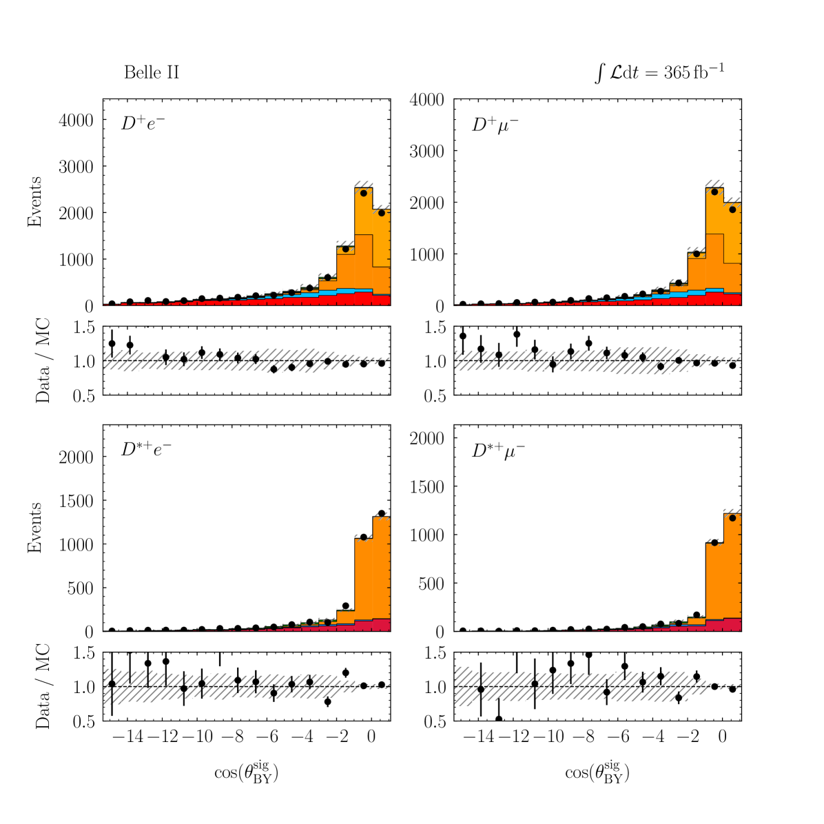
We reconstruct candidates using the Full Event Interpretation (FEI) algorithm [26]. The algorithm constructs candidates from tracks and clusters, using multivariate classifiers and by using a hierarchical approach. The algorithm is trained to identify semileptonic decays and we use it to reconstruct and decay candidates, where the and undergo subsequent hadronic decays. A complete list of decay modes and selection criteria is given in Ref. [43]. Each candidate is assigned a confidence score by the algorithm, ranging from zero to one. Candidates with a confidence score above are selected. To suppress signal-side semitauonic decays in the candidates, the lepton momentum in the center-of-mass (c.m.) frame must exceed GeV. The cosine of the angle between the meson’s momentum and its visible decay products in the c.m. frame is defined as
| (2) |
where is the beam energy, is the meson mass, and is its momentum, computed from and . Here represents the system of visible decay products. For correctly reconstructed semileptonic decays with a single undetected neutrino, lies within , but resolution effects and final-state radiation shift it beyond this range. Semitauonic decays with multiple missing neutrinos have on average large negative values of . All candidates are required to have in the range , reducing the fraction of semitauonic decays among selected candidates to below .
Background from production is suppressed using Fox-Wolfram moments [44], which are constructed from a superposition of spherical harmonics using tracks and clusters. The tracks used in the calculation of Fox–Wolfram moments must lie within the CDC acceptance region, have transverse momenta above GeV, and satisfy cm and cm. The less stringent requirement enhances discrimination against backgrounds by including tracks with larger longitudinal displacements, which are more characteristic of signal decays and improve event shape information. We apply a cut on the ratio of the second-order to the zeroth-order Fox–Wolfram moments, with the second-order moment quantifying deviations of the energy flow from isotropy and the zeroth-order moment reflecting the event’s spherical geometry. Higher ratios indicate a more collimated structure typical of events. Therefore, we require this ratio to be less than 0.4 to reduce the background.
On average, approximately 2.02 candidates per event are reconstructed in the events that passed the selection criteria. From these, we select the candidate with the highest classifier value.
We reconstruct candidates in two final states: and candidates are formed from tracks and clusters not associated with the candidate. Exactly one charged lepton candidate is required. The signal-side lepton is required to have a charge opposite to the lepton and is identified using a likelihood-based score that incorporates information from several subdetectors. Electron identification relies on information from the ECL, CDC, TOP, and ARICH, with the most important discriminant being the ratio of reconstructed ECL energy to the estimated track momentum, which is expected to be close to unity for electrons. Electron candidates must have momenta above GeV, with a loose LID score selection. We correct the electron energy for bremsstrahlung losses by adding back ECL clusters that are near the tracks, following the methodology of Ref. [24]. Muons are identified by extrapolating tracks to the KLM, where the likelihood is primarily constructed from the longitudinal penetration depth and transverse scattering of the extrapolated track. Muon candidates must have momenta above GeV, with a stringent LID score requirement. The efficiency for correctly identifying electrons is 98.7% (99.7%) in semitauonic (semileptonic) events, with a misidentification rate such that only 1% of pions or kaons pass this requirement. The efficiency for correctly identifying muons is 79.3% (86.3%) in semitauonic (semileptonic) events, with only 5% of pions or kaons satisfying the selection.
Neutral pion () candidates are reconstructed from pairs of ECL clusters not associated with any tracks with an invariant mass between and MeV. To suppress background, clusters must have energies above , , or GeV in the forward, barrel, and backward regions, respectively. Each cluster must consist of multiple crystals, lie within the CDC angular acceptance, and have a measured time within ns of the expected event time. A multivariate classifier is constructed from electromagnetic cluster shape quantities and combined with the photon’s distance to the nearest track to distinguish real photons from clusters originating from hadronic showers. More details can be found in Ref. [23].
Neutral kaon () candidates are reconstructed from pairs of charged particles, each of which is assigned a pion mass hypothesis, whose combined invariant mass lies between and MeV and which can be fit to a common vertex. The flight distance must be positive, the significance of the displacement between the point of closest approach and the IP must exceed , and the cosine of the angle between the momentum and vertex position vector must be greater than . The displacement significance, defined as the separation divided by its uncertainty, distinguishes true candidates from random combinations of tracks.
The decays of mesons are reconstructed in modes with large branching fractions and high purities. For the final state, we include , , , , , and . For the final state, where only the decay is used, we include , , , , , , and . All candidates must have a reconstructed invariant mass within of the nominal mass [41], where refers to the resolution of the mass peak.
For the reconstruction of candidates, each candidate is combined with a single charged track, assumed to be a pion. Candidates are required to have a mass difference between 130 and 160 MeV, corresponding to 2.8 times the resolution. An additional vertex fit is performed on each candidate to update its momentum. Using MC simulation, we estimate that for true candidates, the slow pion is correctly identified in 71% of cases.
The construction of candidates is achieved by combining and candidates. The requirement selects semitauonic and semileptonic final states, with approximately 5% of semitauonic signal events falling outside this range on the negative end.
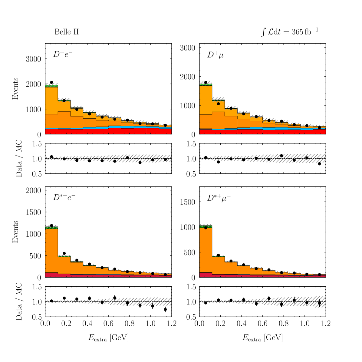
Finally, and candidates are combined to form candidates, requiring no additional charged tracks in the event. We demand that and are of opposite flavor and reject events in which one mixed, as such events possess lower purity. On average, fewer than candidates remain per event after applying the selection criteria, and we select a single candidate per event based on the highest signal-side vertex fit -value. The unassigned energy in the calorimeter of the selected candidate, , is calculated by summing clusters not associated with any particles used in the reconstruction. Two multivariate algorithms, described in Ref. [45] and based on the FastBDT classifier [46], remove contributions from beam background and hadronic split-offs, by utilizing features based on timing, energy spread, scintillation pulse shape, and cluster localization in the ECL. Clusters added as bremsstrahlung corrections to tracks are excluded. From correctly reconstructed events we expect values of near zero, while background events typically exhibit higher values. We only retain events with GeV.
Appendix A provides more details on the differences of the signal and tag-side selection and reconstruction.
V Multivariate Classification
Signal extraction is performed using a multiclass classification algorithm that differentiates semitauonic signal, semileptonic signal, and background events. The model employs gradient-boosted decision trees (BDTs), where each tree corrects the errors of the previous ones to improve classification. Further details can be found in Ref. [47].
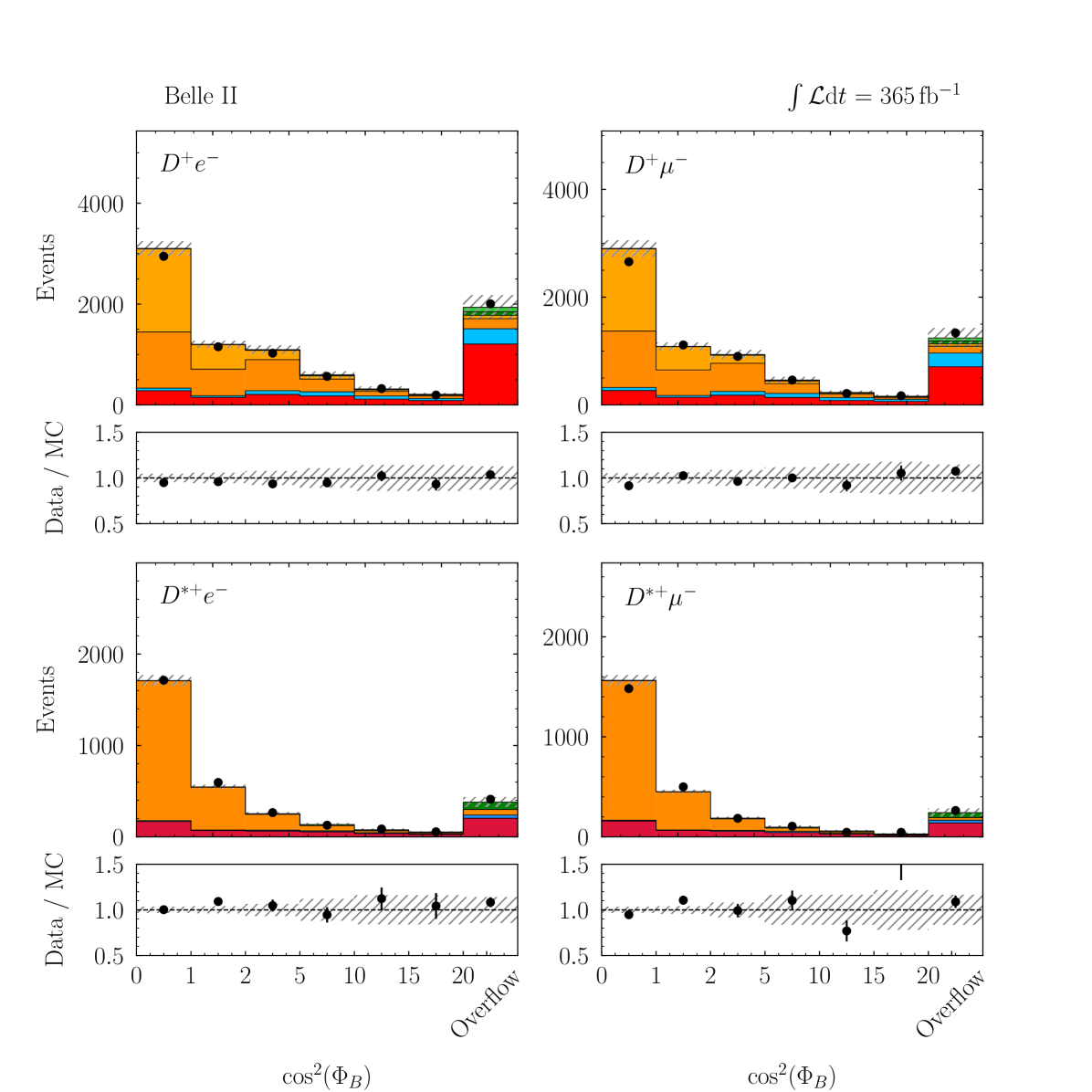
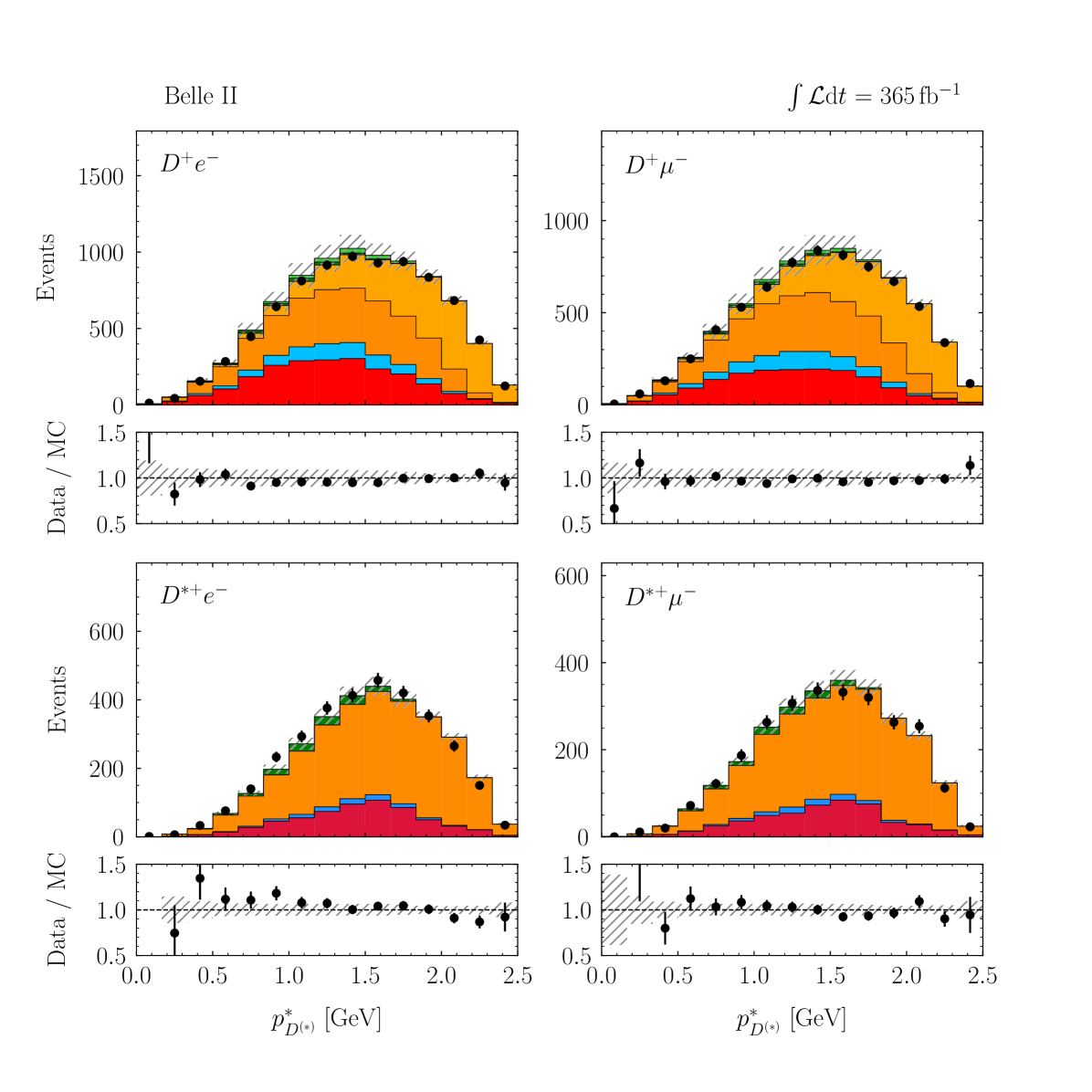
The BDT is trained on five input variables. The most discriminating variable is of the candidate, followed by the unassigned energy in the calorimeter, . The third most important variable, , is defined as
| (3) |
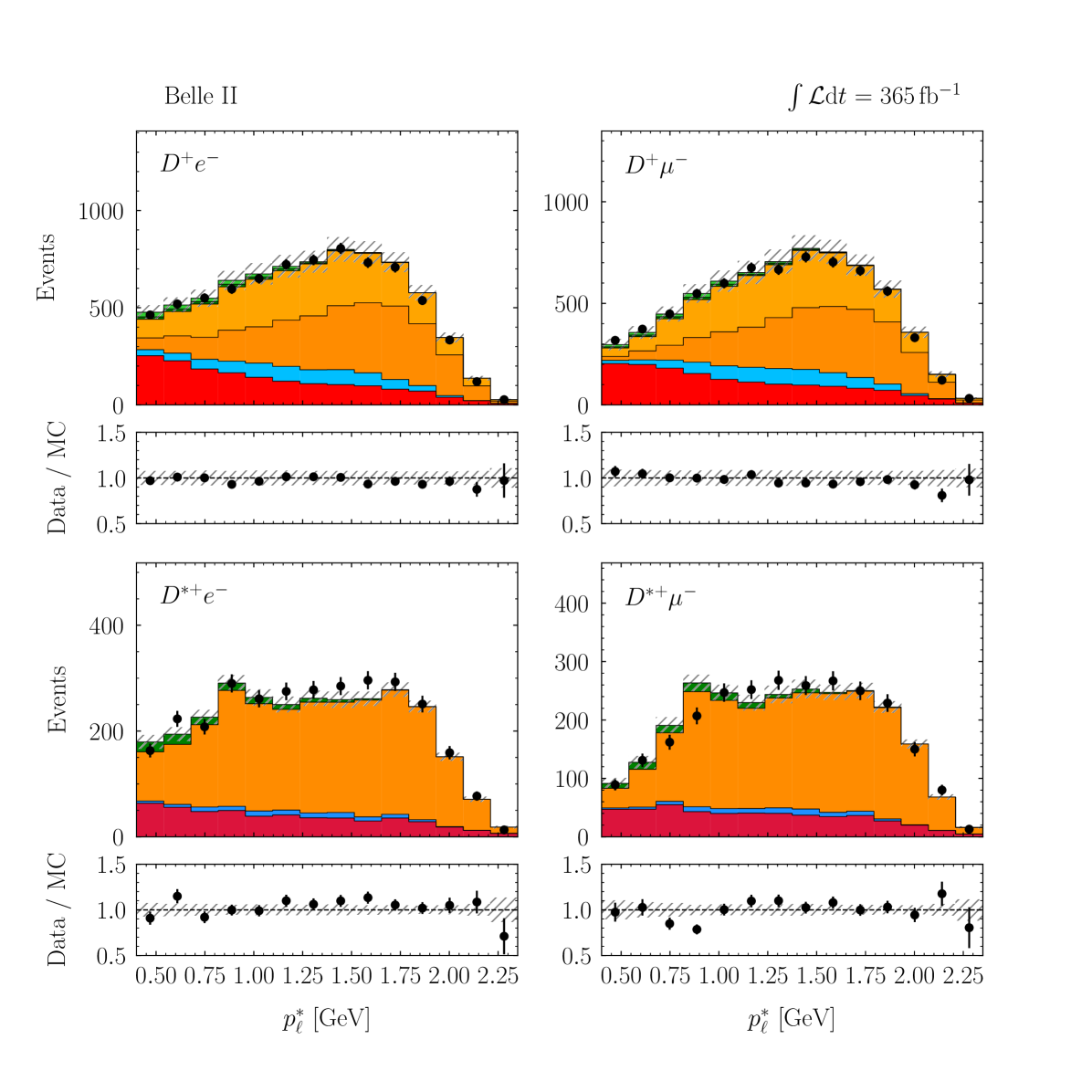
It combines from both the and candidates with the angle between their momenta. For correctly reconstructed semileptonic and candidates, each with a single missing neutrino, is expected to take values between zero and one. Events with multiple missing neutrinos, such as semitauonic decays or misreconstructed events, tend to have larger values. The fourth and fifth most important input variables are the center-of-mass momenta of the () and lepton () candidates, respectively. These variables help distinguish semitauonic, semileptonic, and background events based on the different phase space available in each case. Figure 1 shows the five input variables for and candidates with electrons and muons combined. A good separation of all three event types can be obtained between semileptonic and semitauonic signal decays in , , , and , whereas is very powerful at separating semileptonic and semitauonic signal from other semileptonic processes or backgrounds. The three resulting classification scores are denoted as , , and for semitauonic, semileptonic, and background events, respectively.

VI Fitting Procedure
We extract the signal using a binned two-dimensional log-likelihood fit to the variables and . We consider four categories of events: , , , and candidates. The likelihood is implemented using the pyhf package [48, 49]. The total likelihood function has the form
| (4) |
with the individual category likelihoods and nuisance-parameter (NP) constraints . The product in Eq. 4 runs over all categories and independent uncertainty sources , respectively. The role of the NP constraints is detailed in Section VII. Each category likelihood is defined as the product of individual Poisson distributions ,
| (5) |
with denoting the number of observed data events and the total number of expected events in a given bin . The number of expected events in a given bin, , is estimated using simulated events. It is given by
| (6) |
where is the total number of events from a given process with a fraction of such events being reconstructed in the bin . The values of and and the sum of semileptonic signal decays from electrons and muons are used to determine the number of semitauonic decays via
| (7) |
where and denote the efficiencies of semitauonic and semileptonic signal decays from electrons and muons.
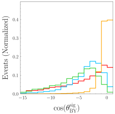
The factor of in Eq. 6 accounts for the definition of the semileptonic signal, which includes both electron and muon final states. We implement a non-uniform binning scheme in both dimensions, increasing granularity in regions where the classifier is most sensitive to semitauonic events and as well as other semileptonic gap backgrounds. In contrast, the region dominated by semileptonic events is binned more coarsely, as these events are readily identifiable. Figure 2 shows the binning structure for semitauonic and semileptonic events, for the background category from and gap modes, and for other backgrounds.
The likelihood (Eq.4) is numerically maximized to fit the values of the different components, , using the observed events. This maximization is performed with the iMinuit package[50]. The ten parameters of interest we determine are:
-
•
and (2 parameters, shared between and channels);
-
•
Normalizations of and events (2 parameters, shared between and channels);
-
•
Background from and semileptonic gap events (2 parameters; shared between and channels);
-
•
Number of other or continuum background events (4 parameters; one for each fit category).
We also test LFU between electrons and muons for the semileptonic signal modes. For this we modify the fit setup by introducing four normalization parameters for each of the four decays of interest and modify Eq. 7 accordingly.
To validate the fit procedure, we generated ensembles of pseudoexperiments for different input and values. Fits to these ensembles show no biases in central values and no under- or overcoverage of determined confidence intervals. Assuming SM values for and , we expect significances of 3.9 and 7.0 standard deviations, respectively.
VII Systematic Uncertainties
Several systematic uncertainties affect the measured ratios of and , and Table 1 provides a summary. The effect of systematic uncertainties is directly incorporated into the likelihood function. We distinguish between additive and multiplicative uncertainties: Additive uncertainties affect the signal and background template shapes, whereas multiplicative uncertainties affect efficiencies or branching fractions of semitauonic and semileptonic signal events. A vector of NPs, , is introduced and each NP is constrained in the likelihood Eq. 4 using a standard normal distribution with denoting an independent uncertainty source or if applicable Poisson constraints.
A brief summary of each significant uncertainty source follows, ordered by their importance:
The dominant uncertainty arises due to the finite size of the simulated data samples and is estimated using the “Barlow-Beeston Lite” method [49], introducing Poisson constraints to correctly treat sparsely populated bins.
The next largest uncertainty stems from the limited knowledge on the composition and modeling of the semileptonic gap processes. To account for the former, we assign a 100% uncertainty to their branching fractions. The latter is addressed by varying the heavy-quark-symmetry-based form factors independently for each assumed gap process, using the uncertainties and correlations provided in Refs. [39, 40] for the broad states. Due to the larger contamination, their impact is more pronounced in the channel than in the channel, translating into a larger systematic uncertainty for .
In contrast, the branching fractions and modeling of resonant decays are better constrained experimentally [51] and we vary the form factors of the broad and narrow states using the uncertainties and correlations provided in Refs. [39, 40].
Lepton identification impacts the precision of and due to the limited size and systematic uncertainties of the calibration samples used to correct discrepancies between data and Monte Carlo simulations. These effects influence both correctly identified leptons and misidentified leptons (“fakes”). The contribution of misidentified background events is larger in the signal-enriched regions of the channels compared to the channels, resulting in a higher uncertainty in .
We assign a track reconstruction efficiency uncertainty of 0.3% per track for kaon, pion, and lepton tracks, reflecting the imperfect knowledge of the track-reconstruction efficiency. This uncertainty is estimated using a control sample of events and is assumed to be fully correlated across all tracks. The slow-pion efficiency for momenta less than 0.2 GeV is corrected relative to the tracking efficiency at momenta larger than 0.2 GeV in the laboratory frame. We study decays to determine corrections for three momentum bins spanning GeV. The associated statistical and systematic uncertainties of the correction weights affect the and and are evaluated using variations of the correction weights, taking into account their correlations.
A systematic uncertainty also arises from the modeling of the BDT input variables. The most significant mis-modeling is observed in the negative region of the distribution of the candidate. To estimate the impact of this mis-modeling, MC samples are reweighted to data, with event weights derived from a linear spline fit to the data-to-MC ratio as a function of . This reweighting is done separately for each of the four categories, yielding distinct spline fits. The event weights are then used to construct a fit, with each template normalized to the nominal fit event count to isolate shape effects. Two approaches were investigated: first, reweighting data while fitting with nominal templates, and second, reweighting the fit templates while fitting to nominal data. We use the larger shift to assess the uncertainty.
The uncertainty on the form factors of semitauonic and semileptonic signal are evaluated by using the eigenvariations provided in Ref. [6]. In addition, we assign the difference in central value between the parametrization of Ref. [6] and Refs. [52, 53] for semileptonic signal and Ref. [54] for semitauonic signal events, using the information from Refs. [55, 56].
Finally, we assign a 10% uncertainty to the fraction of continuum events in the background, based on the observed difference in efficiency between off-resonance data and the expected continuum contribution.
| Systematic Uncertainty | ||
|---|---|---|
| Additive | ||
| MC sample size | 0.033 (8.0%) | 0.014 (4.7%) |
| Gap | 0.027 (6.4%) | 0.001 (0.1%) |
| LID efficiency () | 0.022 (5.1%) | 0.001 (0.1%) |
| Fake rates () | 0.012 (2.9%) | 0.003 (0.9%) |
| from | 0.003 (0.7%) | 0.001 (0.1%) |
| Continuum fraction | 0.002 (0.6%) | 0.001 (0.2%) |
| / FFs | 0.002 (0.5%) | 0.002 (0.7%) |
| Gap FFs | 0.002 (0.5%) | 0.001 (0.2%) |
| 0.002 (0.5%) | 0.001 (0.1%) | |
| FFs | 0.001 (0.3%) | 0.001 (0.2%) |
| BDT modeling | 0.001 (0.3%) | 0.001 (0.2%) |
| LID efficiency () | 0.001 (0.1%) | 0.001 (0.2%) |
| Fake rates () | 0.001 (0.1%) | 0.001 (0.1%) |
| Total Additive Uncertainty | 0.050 (12%) | 0.015 (4.8%) |
| Multiplicative | ||
| / FFs | 0.009 (2.1%) | 0.011 (3.5%) |
| MC sample size | 0.007 (1.7%) | 0.004 (1.2%) |
| LID efficiency () | 0.001 (0.2%) | 0.001 (0.2%) |
| 0.001 (0.2%) | 0.001 (0.2%) | |
| LID efficiency () | 0.001 (0.1%) | 0.001 (0.1%) |
| Tracking efficiency | 0.001 (0.1%) | 0.001 (0.1%) |
| from | – (–) | 0.001 (0.2%) |
| Total Multiplicative Uncertainty | 0.012 (2.8%) | 0.011 (3.7%) |
| Total Syst. Uncertainty | 0.051 (12%) | 0.018 (6.2%) |
| Total Stat. Uncertainty | 0.074 (18%) | 0.034 (11%) |
| Total Uncertainty | 0.090 (22%) | 0.039 (13%) |
VIII Results
VIII.1 and

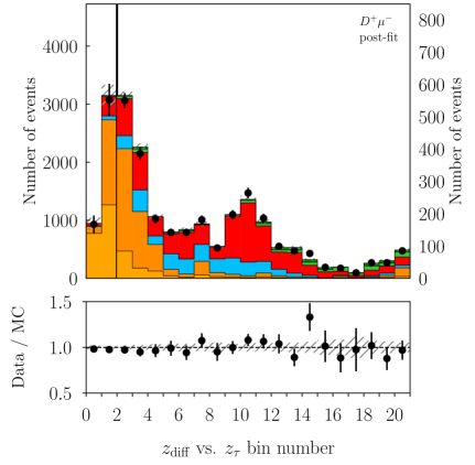
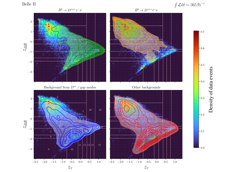
Figure 3 shows the fitted classifier bins for the and categories. We measure
| (8) | |||
| (9) |
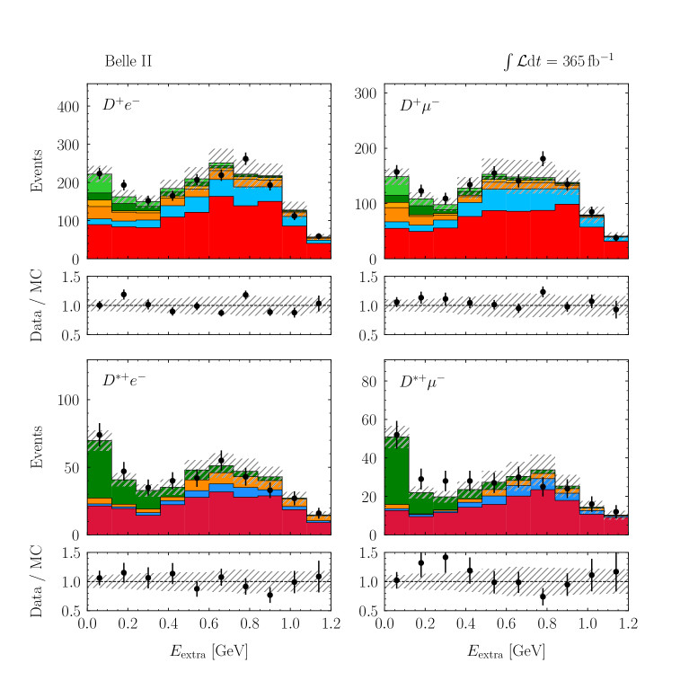
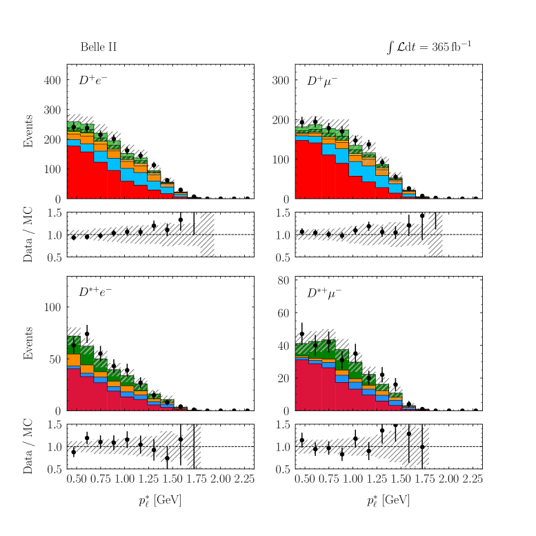
with a correlation of . These values are compatible with the SM predictions of and [2, 3, 4, 5, 6, 7, 8, 9, 10] within 1.7 standard deviations. The p-value of the fit is 8.3% and evaluated using the saturated likelihood method [57]. Figures 4–5 show the distributions of and for the signal enriched bins of the two-dimensional classifier with the post-fit scaling applied. More details can be found in Appendix B.
VIII.2 LFU tests of electrons versus muons
For the ratio of the semileptonic signal branching fractions of electrons to muons we find,
| (10) | ||||
| (11) |
consistent with the expectation of LFU within 1.2 and 1.6 standard deviations, respectively.
VIII.3 Consistency Checks
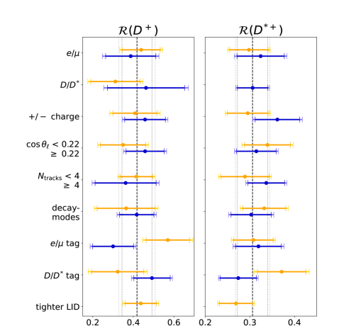
To assess the stability of the result, we determine for various subsamples, fitting them simultaneously to account for correlations in common systematic uncertainties. The tests are summarized in Figure 6. We consider several sample divisions: First, we split by the lepton flavor of the semitauonic and semileptonic signal, fitting separately in the reconstructed electron and muon channels. We also decouple the and fit channels, allowing for an independent extraction of and in the sample, while fitting only in the sample.
The limited number of feed-down signal events results in a large anti-correlation. The obtained () values in the split datasets are consistent with the nominal result with p-values ranging from 10%–78% (20%–88%).
Additional cross-checks involve splitting the data by the charge of the signal lepton and by its polar angle, where the latter is divided at to approximately halve the dataset. We also consider a separation based on the number of reconstructed tracks on the signal side (excluding the lepton). Here, we choose a threshold of four tracks to ensure a balanced division of the dataset.
Beyond that, the dataset is split according to different meson reconstruction modes, selecting alternating modes based on their branching fractions. Furthermore, we divide the dataset based on the decay modes of the tag-side : We partition the dataset by choosing only tag-side semileptonic decays with electrons and with muons, respectively. Second, we further categorize events by distinguishing between tag-side decays with mesons and those with mesons. We also test the stability using a more stringent LID selection and find good agreement between the results.
IX Conclusions
We report measurements of the ratios and and test the predictions of lepton-flavor-universality of the SM. For this we analyzed a data sample, recorded by the Belle II experiment from 2019–2022. Signal events are selected by first reconstructing the companion meson in semileptonic modes using a hierarchical approach. The signal side is analyzed using a multi-class multivariate approach, combining the discriminating power of five variables. The selected events are analyzed using a likelihood fit and we determine
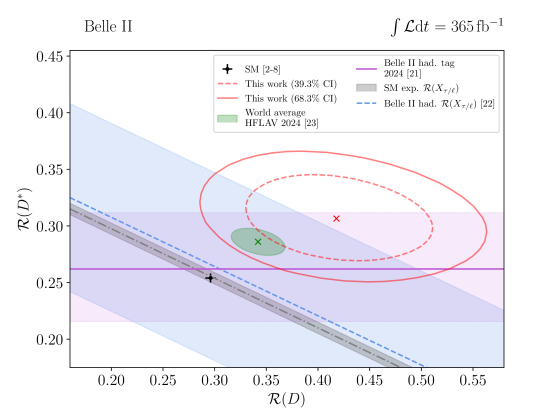
consistent with the SM expectation within 1.7 standard deviations. Figure 7 shows the 2D confidence intervals (CI) and compares this result with the SM expectation and the Belle II measurements Refs. [23, 24], which analyzed an orthogonal data set. Further we present the world average from Ref. [25] and find our results to be consistent with it within 0.6 standard deviations. The uncertainties on the measurements of the ratios are dominated by statistical uncertainties and the largest systematic uncertainty is the limited simulated sample size used to determine efficiencies, train the multi-class classification algorithm, and determine template shapes.
Acknowledgements.
This work, based on data collected using the Belle II detector, which was built and commissioned prior to March 2019, was supported by Higher Education and Science Committee of the Republic of Armenia Grant No. 23LCG-1C011; Australian Research Council and Research Grants No. DP200101792, No. DP210101900, No. DP210102831, No. DE220100462, No. LE210100098, and No. LE230100085; Austrian Federal Ministry of Education, Science and Research, Austrian Science Fund (FWF) Grants DOI: 10.55776/P34529, DOI: 10.55776/J4731, DOI: 10.55776/J4625, DOI: 10.55776/M3153, and DOI: 10.55776/PAT1836324, and Horizon 2020 ERC Starting Grant No. 947006 “InterLeptons”; Natural Sciences and Engineering Research Council of Canada, Compute Canada and CANARIE; National Key R&D Program of China under Contract No. 2024YFA1610503, and No. 2024YFA1610504 National Natural Science Foundation of China and Research Grants No. 11575017, No. 11761141009, No. 11705209, No. 11975076, No. 12135005, No. 12150004, No. 12161141008, No. 12475093, and No. 12175041, and Shandong Provincial Natural Science Foundation Project ZR2022JQ02; the Czech Science Foundation Grant No. 22-18469S and Charles University Grant Agency project No. 246122; European Research Council, Seventh Framework PIEF-GA-2013-622527, Horizon 2020 ERC-Advanced Grants No. 267104 and No. 884719, Horizon 2020 ERC-Consolidator Grant No. 819127, Horizon 2020 Marie Sklodowska-Curie Grant Agreement No. 700525 “NIOBE” and No. 101026516, and Horizon 2020 Marie Sklodowska-Curie RISE project JENNIFER2 Grant Agreement No. 822070 (European grants); L’Institut National de Physique Nucléaire et de Physique des Particules (IN2P3) du CNRS and L’Agence Nationale de la Recherche (ANR) under Grant No. ANR-21-CE31-0009 (France); BMBF, DFG, HGF, MPG, and AvH Foundation (Germany); Department of Atomic Energy under Project Identification No. RTI 4002, Department of Science and Technology, and UPES SEED funding programs No. UPES/R&D-SEED-INFRA/17052023/01 and No. UPES/R&D-SOE/20062022/06 (India); Israel Science Foundation Grant No. 2476/17, U.S.-Israel Binational Science Foundation Grant No. 2016113, and Israel Ministry of Science Grant No. 3-16543; Istituto Nazionale di Fisica Nucleare and the Research Grants BELLE2, and the ICSC – Centro Nazionale di Ricerca in High Performance Computing, Big Data and Quantum Computing, funded by European Union – NextGenerationEU; Japan Society for the Promotion of Science, Grant-in-Aid for Scientific Research Grants No. 16H03968, No. 16H03993, No. 16H06492, No. 16K05323, No. 17H01133, No. 17H05405, No. 18K03621, No. 18H03710, No. 18H05226, No. 19H00682, No. 20H05850, No. 20H05858, No. 22H00144, No. 22K14056, No. 22K21347, No. 23H05433, No. 26220706, and No. 26400255, and the Ministry of Education, Culture, Sports, Science, and Technology (MEXT) of Japan; National Research Foundation (NRF) of Korea Grants No. 2016R1-D1A1B-02012900, No. 2018R1-A6A1A-06024970, No. 2021R1-A6A1A-03043957, No. 2021R1-F1A-1060423, No. 2021R1-F1A-1064008, No. 2022R1-A2C-1003993, No. 2022R1-A2C-1092335, No. RS-2023-00208693, No. RS-2024-00354342 and No. RS-2022-00197659, Radiation Science Research Institute, Foreign Large-Size Research Facility Application Supporting project, the Global Science Experimental Data Hub Center, the Korea Institute of Science and Technology Information (K24L2M1C4) and KREONET/GLORIAD; Universiti Malaya RU grant, Akademi Sains Malaysia, and Ministry of Education Malaysia; Frontiers of Science Program Contracts No. FOINS-296, No. CB-221329, No. CB-236394, No. CB-254409, and No. CB-180023, and SEP-CINVESTAV Research Grant No. 237 (Mexico); the Polish Ministry of Science and Higher Education and the National Science Center; the Ministry of Science and Higher Education of the Russian Federation and the HSE University Basic Research Program, Moscow; University of Tabuk Research Grants No. S-0256-1438 and No. S-0280-1439 (Saudi Arabia), and Researchers Supporting Project number (RSPD2025R873), King Saud University, Riyadh, Saudi Arabia; Slovenian Research Agency and Research Grants No. J1-9124 and No. P1-0135; Ikerbasque, Basque Foundation for Science, State Agency for Research of the Spanish Ministry of Science and Innovation through Grant No. PID2022-136510NB-C33, Spain, Agencia Estatal de Investigacion, Spain Grant No. RYC2020-029875-I and Generalitat Valenciana, Spain Grant No. CIDEGENT/2018/020; The Knut and Alice Wallenberg Foundation (Sweden), Contracts No. 2021.0174 and No. 2021.0299; National Science and Technology Council, and Ministry of Education (Taiwan); Thailand Center of Excellence in Physics; TUBITAK ULAKBIM (Turkey); National Research Foundation of Ukraine, Project No. 2020.02/0257, and Ministry of Education and Science of Ukraine; the U.S. National Science Foundation and Research Grants No. PHY-1913789 and No. PHY-2111604, and the U.S. Department of Energy and Research Awards No. DE-AC06-76RLO1830, No. DE-SC0007983, No. DE-SC0009824, No. DE-SC0009973, No. DE-SC0010007, No. DE-SC0010073, No. DE-SC0010118, No. DE-SC0010504, No. DE-SC0011784, No. DE-SC0012704, No. DE-SC0019230, No. DE-SC0021274, No. DE-SC0021616, No. DE-SC0022350, No. DE-SC0023470; and the Vietnam Academy of Science and Technology (VAST) under Grants No. NVCC.05.12/22-23 and No. DL0000.02/24-25. These acknowledgements are not to be interpreted as an endorsement of any statement made by any of our institutes, funding agencies, governments, or their representatives. We thank the SuperKEKB team for delivering high-luminosity collisions; the KEK cryogenics group for the efficient operation of the detector solenoid magnet and IBBelle on site; the KEK Computer Research Center for on-site computing support; the NII for SINET6 network support; and the raw-data centers hosted by BNL, DESY, GridKa, IN2P3, INFN, and the University of Victoria.References
- Bernlochner et al. [2022a] F. U. Bernlochner, M. F. Sevilla, D. J. Robinson, and G. Wormser, Rev. Mod. Phys. 94, 015003 (2022a), arXiv:2101.08326 [hep-ex] .
- Bigi and Gambino [2016] D. Bigi and P. Gambino, Phys. Rev. D 94, 094008 (2016), arXiv:1606.08030 [hep-ph] .
- Gambino et al. [2019] P. Gambino, M. Jung, and S. Schacht, Phys. Lett. B 795, 386 (2019), arXiv:1905.08209 [hep-ph] .
- Bordone et al. [2020] M. Bordone, M. Jung, and D. van Dyk, Eur. Phys. J. C 80, 74 (2020), arXiv:1908.09398 [hep-ph] .
- Martinelli et al. [2022] G. Martinelli, S. Simula, and L. Vittorio, Phys. Rev. D 105, 034503 (2022), arXiv:2105.08674 [hep-ph] .
- Bernlochner et al. [2022b] F. U. Bernlochner, Z. Ligeti, M. Papucci, M. T. Prim, D. J. Robinson, and C. Xiong, Phys. Rev. D 106, 096015 (2022b), arXiv:2206.11281 [hep-ph] .
- Ray and Nandi [2024] I. Ray and S. Nandi, J. High Energ. Phys. 22, 022 (2024).
- Y. Aoki, T. Blum, G. Colangelo et al. [2022] Y. Aoki, T. Blum, G. Colangelo et al., Eur. Phys. J. C 82, 869 (2022), arXiv:2111.09849 [hep-lat] .
- Lees et al. [2019] J. P. Lees et al. (BaBar), Phys. Rev. Lett. 123, 091801 (2019), arXiv:1903.10002 [hep-ex] .
- Martinelli et al. [2024] G. Martinelli, S. Simula, and L. Vittorio, Eur. Phys. J. C 84, 400 (2024).
- Lees et al. [2012] J. P. Lees et al. (BaBar), Phys. Rev. Lett. 109, 101802 (2012), arXiv:1205.5442 [hep-ex] .
- Lees et al. [2013] J. P. Lees et al. (BaBar), Phys. Rev. D 88, 072012 (2013), arXiv:1303.0571 [hep-ex] .
- Huschle et al. [2015] M. Huschle et al. (Belle), Phys. Rev. D 92, 072014 (2015), arXiv:1507.03233 [hep-ex] .
- Sato et al. [2016] Y. Sato et al. (Belle), Phys. Rev. D 94, 072007 (2016), arXiv:1607.07923 [hep-ex] .
- Hirose et al. [2017] S. Hirose et al. (Belle), Phys. Rev. Lett. 118, 211801 (2017), arXiv:1612.00529 [hep-ex] .
- Hirose et al. [2018] S. Hirose et al. (Belle), Phys. Rev. D 97, 012004 (2018), arXiv:1709.00129 [hep-ex] .
- Caria et al. [2020] G. Caria et al. (Belle), Phys. Rev. Lett. 124, 161803 (2020), arXiv:1910.05864 [hep-ex] .
- Aaij et al. [2018] R. Aaij et al. (LHCb), Phys. Rev. Lett. 120, 121801 (2018), arXiv:1711.05623 [hep-ex] .
- [19] R. Aaij et al. (LHCb), Phys. Rev. Lett. 128, 10.1103/PhysRevLett.128.191803, arXiv:2201.03497 [hep-ex] .
- Aaij et al. [2023a] R. Aaij et al. (LHCb), Phys. Rev. Lett. 131, 111802 (2023a), arXiv:2302.02886 [hep-ex] .
- Aaij et al. [2023b] R. Aaij et al. (LHCb), Phys. Rev. D 108, 012018 (2023b), arXiv:2305.01463 [hep-ex] .
- Aaij et al. [2025] R. Aaij et al. (LHCb), (2025), arXiv:2501.14943 [hep-ex] .
- Adachi et al. [2024a] I. Adachi et al. (Belle II), Phys. Rev. D 110, 072020 (2024a).
- Adachi et al. [2024b] I. Adachi et al. (Belle II), Phys. Rev. Lett. 132, 211804 (2024b), arXiv:2311.07248 [hep-ex] .
- Banerjee et al. [2024] S. Banerjee et al. (Heavy Flavor Averaging Group (HFLAV)), (2024), arXiv:2411.18639 [hep-ex] .
- Keck et al. [2019] T. Keck et al., Comput. Softw. Big Sci. 3, 6 (2019), arXiv:1807.08680 [hep-ex] .
- Akai et al. [2018] K. Akai, K. Furukawa, and H. Koiso (SuperKEKB), Nucl. Instrum. Meth. A 907, 188 (2018), arXiv:1809.01958 [physics.acc-ph] .
- Abe et al. [2010] T. Abe et al. (Belle II), (2010), arXiv:1011.0352 [physics.ins-det] .
- Abashian et al. [2002] A. Abashian et al., Nucl. Instrum. Meth. A 479, 117 (2002), also see detector section in J. Brodzicka et al., Prog. Theor. Exp. Phys. 2012, 04D001 (2012).
- Lange [2001] D. J. Lange, Nucl. Instr. and. Meth. A 462, 152 (2001).
- Jadach et al. [2000] S. Jadach, B. F. L. Ward, and Z. Was, Comput. Phys. Commun. 130, 260 (2000), arXiv:hep-ph/9912214 .
- Sjöstrand et al. [2015] T. Sjöstrand et al., Comput. Phys. Commun. 191, 159 (2015), arXiv:1410.3012 [hep-ph] .
- Barberio et al. [1991] E. Barberio, B. van Eijk, and Z. Wąs, Comput. Phys. Commun. 66, 115 (1991).
- Agostinelli et al. [2003] S. Agostinelli et al. (GEANT4), Nucl. Instrum. Meth. A 506, 250 (2003).
- Glattauer et al. [2016] R. Glattauer et al. (Belle), Phys. Rev. D 93, 032006 (2016), arXiv:1510.03657 [hep-ex] .
- Waheed et al. [2019] E. Waheed et al. (Belle), Phys. Rev. D 100, 052007 (2019), [Erratum: Phys. Rev. D 103, 079901 (2021)], arXiv:1809.03290 [hep-ex] .
- Bernlochner et al. [2020] F. U. Bernlochner, S. Duell, Z. Ligeti, M. Papucci, and D. J. Robinson, Eur. Phys. J. C 80, 883 (2020).
- Amhis et al. [2023] Y. S. Amhis et al. (HFLAV), Phys. Rev. D 107, 052008 (2023), arXiv:2206.07501 [hep-ex] .
- Bernlochner and Ligeti [2017] F. U. Bernlochner and Z. Ligeti, Phys. Rev. D 95, 014022 (2017), arXiv:1606.09300 [hep-ph] .
- Bernlochner et al. [2018] F. U. Bernlochner, Z. Ligeti, and D. J. Robinson, Phys. Rev. D 97, 075011 (2018), arXiv:1711.03110 [hep-ph] .
- Navas et al. [2024] S. Navas et al. (Particle Data Group), Phys. Rev. D 110, 030001 (2024).
- Kuhr et al. [2019] T. Kuhr, C. Pulvermacher, M. Ritter, T. Hauth, and N. Braun (Belle II Framework Software Group), Comput. Softw. Big Sci. 3, 1 (2019), arXiv:1809.04299 [physics.comp-ph] .
- Keck [2017a] T. Keck, Machine learning algorithms for the Belle II experiment and their validation on Belle data, Ph.D. thesis, Karlsruher Institut für Technologie (KIT) (2017a).
- Fox and Wolfram [1978] G. C. Fox and S. Wolfram, Phys. Rev. Lett. 41, 1581 (1978).
- Cheema [2024] P. Cheema, EPJ Web Conf. 295, 09035 (2024).
- Keck [2017b] T. Keck, Comput. Softw. Big Sci. 1, 2 (2017b).
- Pedregosa et al. [2011] F. Pedregosa et al., Journal of Machine Learning Research 12, 2825 (2011).
- Heinrich et al. [2021] L. Heinrich, M. Feickert, G. Stark, and K. Cranmer, Journal of Open Source Software 6, 2823 (2021).
- Cranmer et al. [2012] K. Cranmer, G. Lewis, L. Moneta, A. Shibata, and W. Verkerke (ROOT), HistFactory: A tool for creating statistical models for use with RooFit and RooStats, Tech. Rep. (New York U., New York, 2012).
- Moneta et al. [2011] L. Moneta, K. Cranmer, D. Baskakov, G. Stark, and W. K. Tung, (2011), arXiv:1101.0423 [physics.data-an] .
- Workman et al. [2022] R. L. Workman et al. (Particle Data Group), PTEP 2022, 083C01 (2022).
- Boyd et al. [1996] C. G. Boyd, B. Grinstein, and R. F. Lebed, Nucl. Phys. B 461, 493 (1996), arXiv:hep-ph/9508211 .
- Boyd et al. [1997] C. G. Boyd, B. Grinstein, and R. F. Lebed, Phys. Rev. D 56, 6895 (1997), arXiv:hep-ph/9705252 .
- Caprini et al. [1998] I. Caprini, L. Lellouch, and M. Neubert, Nucl. Phys. B530, 153 (1998), arXiv:hep-ph/9712417 [hep-ph] .
- Fajfer et al. [2012] S. Fajfer, J. F. Kamenik, and I. Nisandzic, Phys. Rev. D 85, 094025 (2012), arXiv:1203.2654 [hep-ph] .
- Tanaka and Watanabe [2010] M. Tanaka and R. Watanabe, Phys. Rev. D 82, 034027 (2010), arXiv:1005.4306 [hep-ph] .
- Baker and Cousins [1984] S. Baker and R. D. Cousins, Nucl. Instrum. Meth. 221, 437 (1984).
Appendix A Selections
Tables 2 and 3 summarize the differences in the tag-side and signal-side reconstruction and the reconstructed decay modes. In the table, refers to the lepton momentum in the laboratory frame; LID refers to the likelihood-based variables used for lepton identification; denotes the energy of the ECL clusters of the photon () candidate; denotes the cosine of the angle between the momentum vector and the vector defined by the reconstructed vertex. In addition, , , , and are the invariant masses of the reconstructed neutral pion, , , and mesons, respectively, while refers to their masses determined in [41]. The parameter is the width of the mass peak as determined from a Gaussian fit and represents the energy release in the particle decay. The classifier output from the tag-side reconstruction algorithm is denoted by .
Table 4 lists the ratios of efficiencies of semitauonic and semileptonic events for the four categories.
| Selection | ||
| tracks | except for from : | |
| cm, cm | cm, cm | |
| within CDC angular acceptance with hit | ||
| LID | ||
| GeV | GeV | |
| LID | ||
| GeV | GeV | |
| forward: GeV | forward: GeV | |
| barrel: GeV | barrel: GeV | |
| backward: GeV | backward: GeV | |
| crystal | ||
| within CDC angular acceptance | ||
| measured time within ns of exp. event time | ||
| for candidates: | ||
| optimized requirement based on the distance to the | ||
| nearest track and a shower-shape classifier | ||
| GeV GeV | GeV GeV | |
| GeV GeV | GeV GeV | |
| flight distance | ||
| significance of distance | ||
| GeV GeV | ||
| with GeV | ||
| and GeV | ||
| GeV | ||
| GeV | ||
| GeV | GeV GeV | |
| cand. with largest | cand. with largest -value from vertex fit |
| Decay mode | tag side | signal side |
|---|---|---|
| - | ||
| - | ||
| - | ||
| - | ||
| - | ||
| - | ||
| - | ||
| - | ||
| - | ||
| - | ||
| - | ||
| - | ||
| - | ||
| - | ||
| - |
| Category | ||||
|---|---|---|---|---|
Appendix B Fit Details
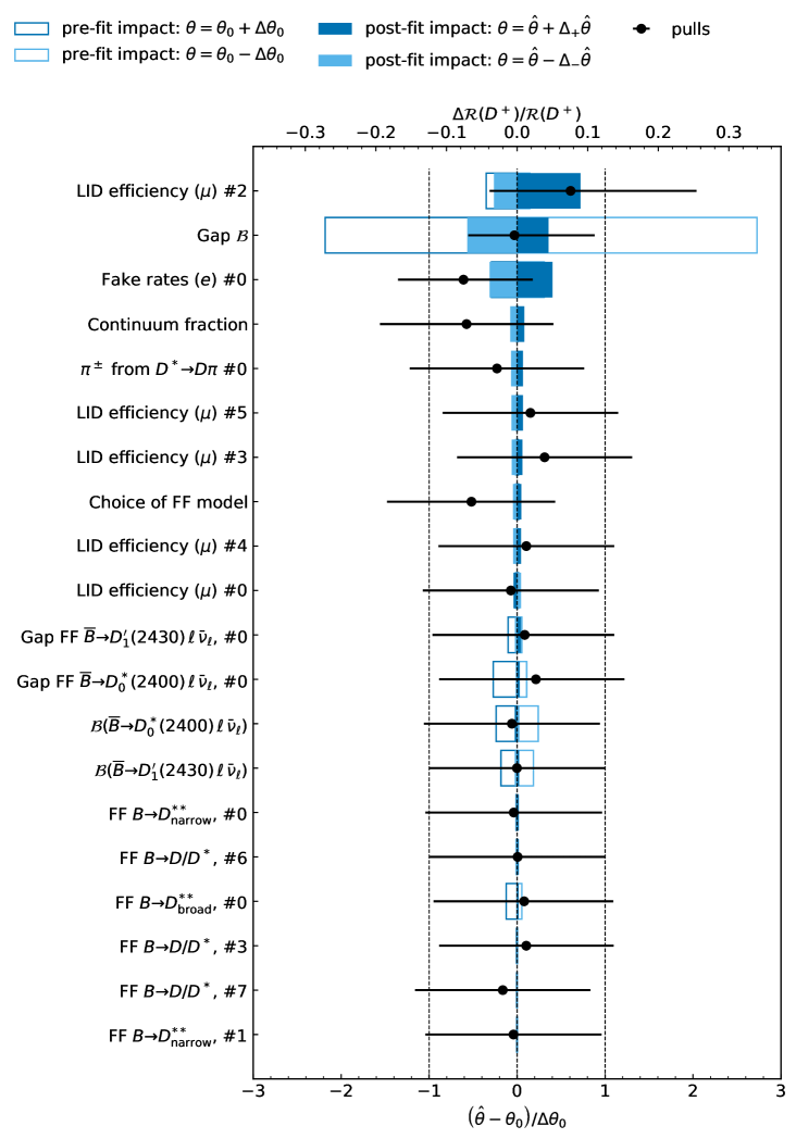
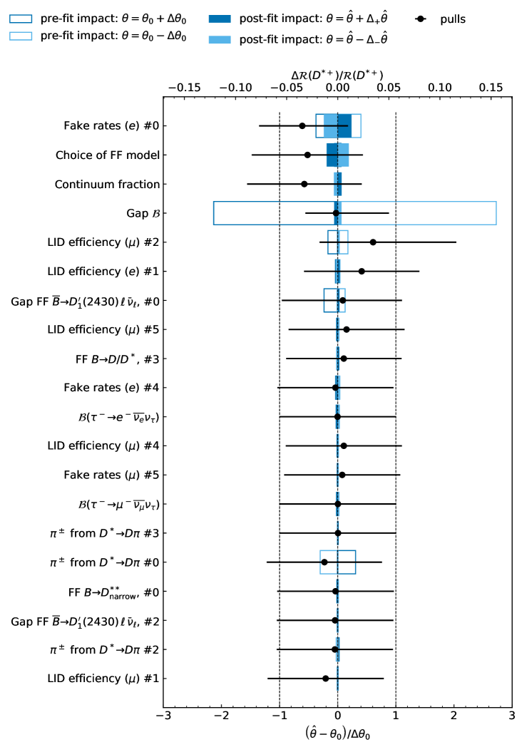
Figure 8 shows the leading 20 systematic uncertainties on and , excluding the dominant systematic uncertainty due to the limited MC sample size. If stated, the number (#) indicates the eigendirection of the uncertainty source. The uncertainty “Choice of FF model” parametrizes the impact of changing the semitauonic and semileptonic signal form factor parameterization, cf. Section VII. Within the FF uncertainties for the resonances, we distinguish between resonances ( and ) and resonances ( and ) as they are described by different parametrizations due to their varying decay widths.
The pull is defined as the difference of the post-fit value () with respect to the nominal input value of the nuisance parameter (), and normalized with the post-fit uncertainty (). The sizes of the error bars on the pulls correspond to the asymmetric confidence intervals obtained from the likelihood profile.
Also shown are the impacts of the relative uncertainties and on the determined ratios. We estimate the pre-fit impact by analyzing how variations in the NP affect the POI, independent of the other fitted parameters: In order to isolate the specific contribution of the NP, we construct an Asimov dataset in which the NP under investigation is maintained at its initial value, while all other parameters are set to their best-fit values obtained from the nominal fit. This dataset is then refitted, keeping all parameters except the respective POI ( or ) fixed to their best-fit values, while shifting the NP to , where denotes its pre-fit uncertainty. The pre-fit impact is then quantified as the relative change in the POI compared to a reference POI value, determined in the same way with the NP set at its initial value.
The post-fit impact is defined as the relative deviation of the POI from its nominal value, considering only post-fit systematic variations. To evaluate this, the best-fit value of the NP from the nominal fit, , is used and varied within its estimated uncertainties, , where represents the asymmetric uncertainty obtained from the likelihood scan. In this case, only the NP under consideration is fixed, while all other parameters are allowed to vary freely during the fit to real data.
Table 5 lists the yields within each category as calculated from the fit parameters.
| Sample | ||||
|---|---|---|---|---|
| 2519 68 | 2233 61 | |||
| 2486 63 | 2323 58 | 2344 51 | 1961 44 | |
| 191 41 | 155 65 | |||
| 106 14 | 84 11 | 155 19 | 111 14 | |
| 653 112 | 586 102 | 87 55 | 75 46 | |
| and | 2177 145 | 1582 149 | 611 95 | 497 83 |
| Data | 8219 | 6854 | 3241 | 2621 |
Appendix C Post-fit Projections of BDT Input Variables
Figures 9–13 show the distributions of the input variables utilized in the multivariate algorithm used in the signal classification, arranged by their importance in the classifier training.
To evaluate the agreement between simulation and data, the fit templates are scaled to their best-fit values.